| Issue |
A&A
Volume 552, April 2013
|
|
|---|---|---|
| Article Number | A139 | |
| Number of page(s) | 5 | |
| Section | The Sun | |
| DOI | https://doi.org/10.1051/0004-6361/201220358 | |
| Published online | 17 April 2013 | |
Research Note
On the detectability of 57Fe axion-photon mode conversion in the Sun
Space Science Division, Naval Research Laboratory, Code 7684, Washington, DC 20375, USA
e-mail: This email address is being protected from spambots. You need JavaScript enabled to view it.
Received: 10 September 2012
Accepted: 16 March 2013
Abstract
Aims. The purpose of this paper is to assess the feasibility of axion detection by X-ray spectroscopy of the sun.
Methods. We review the theory of axion-photon mode conversion with special attention to axions emitted in the 14.4 keV M1 decay of 57Fe at the solar center. These then mode convert to photons in the outer layers of the solar envelope, and may in principle be detected subsequently as X-rays.
Results. For axion masses above about 10-4 eV, resonant mode conversion at a layer where the axion mass matches the local electron plasma frequency is necessary. For axion masses above about 10-2 eV, this mode conversion occurs too deep in the solar atmosphere for the resulting photon to escape the solar surface and be detected before Compton scattering obscures the line. At the (detectable) axion masses below this, the flux of mode converted photons predicted by axion models appears to be too low for detection to be feasible with current instrumentation. Nonresonant mode conversion for axion masses below 10-4 eV is also plausible, but with still lower predicted fluxes, since the axion coupling constant is related to its mass.
Conclusions. Prospects for meaningful constraints on massive axion parameters from X-ray observations of this transition from the Sun do not appear to be promising. However parameters for massless counterparts (e.g. the “arion”) may still result from such observations. It may mode convert in the outer layers of the solar atmosphere, but is not restricted by this to have a small coupling constant.
Key words: elementary particles / Sun: particle emission / Sun: X-rays, gamma rays
© ESO, 2013
1. Introduction
The basic form of the Lagrangian for the theory of strong interactions known as quantum chromodynamics (QCD) contains a pseudo-scalar term involving the gluon field strength tensor that violates symmetry under the actions of charge and parity reversal (CP violation). One practical consequence of this is the prediction of an electric dipole moment for the neutron in excess of the experimental limits by about ten orders of magnitude. The most generally accepted solution to this problem involves the introduction of a new global chiral symmetry (Peccei & Quinn 1977a,b). Weinberg (1978) and Wilczek (1978) pointed out that such a symmetry, being spontaneously broken, necessitates the existence of a new boson, the axion, with mass in the range 10-12 eV to 1 MeV, depending on the scale at which the global symmetry is broken. The axion mass is related to the symmetry breaking scale, fPQ, by (e.g. Moriyama 1995)  (1)Limits on the axion mass are placed by various astrophysical constraints. There are two most often discussed classes of axion; “hadronic” axions that do not couple to leptons and quarks at tree level (Kim 1979; Shifman et al. 1980) and DFSZ axions that do (Dine et al. 1981; Zhitnitskii 1980). Both types of axion are constrained to have masses less than about 10-3−10-2 eV based on analyses of the neutrino burst from SN 1987A (Burrows et al. 1989; Keil et al. 1997), while hadronic axions may also have a mass of a few eV, bounded from below by treatments of axion trapping in SN 1987A (Burrows et al. 1990) and from above by studies of red giant evolution (Haxton & Lee 1991). Studies of white dwarf cooling and pulsation also indicate DFSZ axion masses of order 10-3 eV (Isern et al. 2010). Cosmological arguments (e.g. Kolb & Turner 1994) give a lower limit on the axion mass in the range 10-6−10-5 eV, with a mass of ~ 10-5 eV supplying the measured cold dark matter density (Erken et al. 2011).
The sun is the only astrophysical object besides SN 1987A from which neutrinos have been directly detected, and so it is natural to consider it also as a potential source of axions. While thermal processes at the solar center produce axions by Compton and Primakoff photoproduction processes, illustrated in Fig. 1, (Chanda et al. 1988), considerable attention has also been devoted to a transition at 14.4 keV in the 57Fe nucleus, which lies in a spectral region with essentially zero background from the nonflaring solar atmosphere. Being an M1 transition, it has a branching ratio for axion emission (DFSZ or hadronic) instead of photon radiation (Haxton & Lee 1991), and has a sufficiently low threshold to allow thermal excitation. An estimate of the axion flux in this line has been given by Andriamonje et al. (2009) as  cm-2 s-1, where
  is the effective axion-nucleon coupling. Moriyama (1995) gives FA = 5.3 × 10⁸(m/1 eV)2 cm-2 s-1 assuming the naive quark model (NQM) where
  . Andriamonje et al. (2009) give
  (in the calculation of the 57Fe M1 axion branching ratio), which would give a flux of FA = 108(m/1 eV)2 cm-2 s-1 but also discuss higher possible values for .
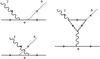 |
Fig. 1 Feynman diagrams illustrating the two Compton scattering diagrams (left) and the Primakoff process (right). |
Andriamonje et al. (2009) describe the CERN Axion Solar Telescope (CAST), designed to detect solar 57Fe axions by observing the 14.4 keV photons produced when the axions mode convert inside the detector. The parameters of CAST; a 9T magnetic field extending over a length of s = 9.26 m, give a product Bs ≃ 8 × 10⁷ G cm, which is smaller than the product of a typical solar magnetic field and density scale height, and so the question of whether 14.4 keV photons might be detectable in the solar spectrum as a signature of in situ axion mode conversion becomes interesting to consider.
2. Axion-photon Interactions
The axion-photon interaction Lagrangian is  (2)where gaγγ is the axion-photon coupling constant, a is the axion field, Fμν is the electromagnetic field tensor and
  is its dual. The product
  , which leads to the final form. Here, E is interpreted as the photon electric field and B the ambient magnetic field. Thus axions only interact with photons when propagating across the ambient magnetic field, and then only with the mode polarized along the magnetic field, known as the ordinary mode.
The effective Lagrangian for an axion-photon system is then  (3)where m is the axion mass and
  is the dielectric tensor in terms of the electron plasma frequency ωp. We are working in the limit of small magnetic fields. By way of contrast, Yoshimura (1988) includes the magnetic field terms in ϵ. The equations of motion are
 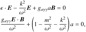 (4)which for nontrivial solutions require
 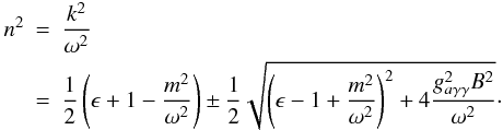 (5)These two solutions represent axion and photon propagation across the magnetic field. We rewrite the photon-axion mass matrix from Eq. (4) in symmetric form as
 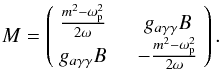 (6)Pre and post multiplying by a rotation matrix,
 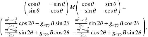 (7)which is diagonal for a mixing angle θ given by
 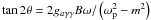 .
.
The evolution of the axion-photon mixed state with time t is described by 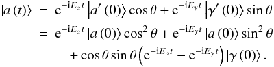 (8)The probability of axion to photon conversion is then
 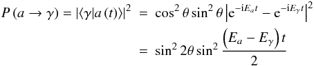 (9)which upon substituting for the mixing angle becomes
 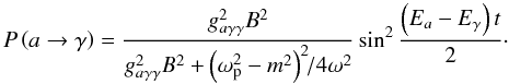 (10)We put
  with
with  given by the two solutions in Eq. (5), and s the distance traveled through the medium. Then
  and
and 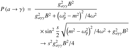 (11)when
  .
.
The forgoing estimate assumed that the electron density is constant. When crossing a resonance, the rapid variation in tan2θ with  first greater than m2 becoming equal and then less than m2, as the axion moves from high density to low density, means that the axion-photon oscillation cannot keep up with the changing Hamiltonian. In this limit, the equations of motion (4) admit solutions in terms of parabolic cylinder functions, yielding an axion transmission probability of
  , (Cairns & Lashmore-Davies 1983; Cally 2006). The corresponding mode conversion probability is then
  (12)and as will be seen below, is generally larger than the nonresonant conversion probability given in Eq. (11).
3. In real numbers ...
We have used natural units, where ħ = c = 1, above. To put variables in units more familiar to solar physicists, we use (Andriamonje et al. 2009)  (13)concentrating on DFSZ axions for the time being, where fPQ is the symmetry breaking scale in GeV, and hence from Eq. (1)
  (14)With these definitions
  (15)where B is given in Gauss, and the conversion probability is
  (16)At a photon energy of 14.4 keV,
  (17)For m > 10-4 eV and s > 108 cm (a typical solar atmosphere scale size) the small angle approximation for the sine in Eq. (11) is not valid. Both terms in Eq. (17) are ≫
  and so unless ωp ≃ m, the conversion probability is significantly reduced from the value in Eq. (16). The electron density at which resonant mode conversion can occur is (see also Yoshimura 1988)
  (18)The electron scattering optical depth between this layer and the solar surface is
 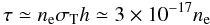 (19)where σT is the Thomson cross section and h ≃ 500 km is the atmosphere density scale height. Figure 2 shows emergent line profiles at the top of the solar atmosphere after traveling through electron scattering optical depths of 0.1, 0.3, 1.0, 3.0, and 5.0, calculated following the treatment of Chandrasekhar (1960) and Münch (1948) for plane parallel atmospheres. As can be seen, the detectable line disappears once τ ~ 5, meaning a maximum density at which detectable mode conversion will occur is ~1017 cm-3, with a maximum detectable axion mass of 1.2 × 10⁻² eV. At higher opacities, a broad Compton scattered feature may still be seen. Figure 3 shows this feature at opacities of 5, 15, 50, and 150. It is visible as a 1–2 keV wide feature out to an opacity of between 15 and 50. This would increase the maximum detectable axion mass to about 4−7 × 10⁻² eV, but would probably require more photons detected due to the broader feature.
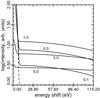 |
Fig. 2 Line profiles of the emergent 14.4 keV 57Fe line, originally emitted as an axion, and mode converted at various optical depths in the solar atmosphere. The electron scattering opacities through which the various profiles have propagated are noted. The dashed curve gives the original unscattered profile. At an opacity of ≃5, the central narrow line has essentially disappeared. |
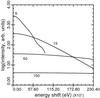 |
Fig. 3 Same as Fig. 1, but for electron scattering opacities of 5, 15, 50, and 150. The τ = 5 curve is truncated for numerical reasons. |
Equation (12) gives the mode conversion probability as P = 7.5 × 10⁻²⁵B2, independent of axion mass. For B ~ 103 G, P ~ 10-18, and the photon flux at earth is 10-10(m/1eV)2 cm-2 s-1, assuming the axion flux calculated by Andriamonje et al. (2009). For axions with mass up to 10-2 eV (the high end of the mass range allowed by SN 1987A observations, and close to the limit allowed by Compton scattering in the solar atmosphere), this leads to a count rate of order 10-11 s-1 in a instrument of effective area 103 cm2 (e.g. NUSTAR; Harrison et al. 2010, 2013); too low for detection. Significantly higher conversion probabilities would be expected in pulsar strength magnetic fields, (Yoshimura 1988; Perna et al. 2012).
For s ~ 108 cm, the argument of the sine in Eq. (11) becomes small for axion masses at the low end of the allowed range, m < 10-4 eV. In this case nonresonant conversion can occur with probability  for B ≃ 103 G and m ≃ 10-4 eV. This yields a flux at earth of mode converted photons of
  . Taking
  as before gives a negligible mode converted photon flux at earth of ~10-19 cm-2 s-1 with m = 10-4 eV. The lower axion mass leads to a significantly lower flux, through its coupling to gaγγ. In hadronic axion models, the parameters gaγγ and are less tightly constrained. Yoshimura (1988) suggests gaγγ may increase by a factor of ten, which would lead to a commensurate increase in the count rates estimated above, though still insufficient to change the conclusions above.
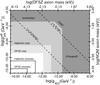 |
Fig. 4 The |
These potential constraints are illustrated in Fig. 4., showing the  parameter space. The top and right hand axes show the corresponding axion masses in the cases of DFSZ axions (Eq. (1)), and those coming from the naive quark model from respectively. The dark region at the top and right indicates the region ruled out by CAST (Andriamonje et al. 2009), and other constraints discussed therein. The dashed contour below this indicates the where this limit moves with the nondetection of a count rate of 10-5 s-1 by NUSTAR (a flux of 10-8 photons cm-2 s-1, and about 10 times the background count rate in this line estimated from Table 2 in Harrison et al. 2013) for resonant axion-photon mode conversion. The shaded contours indicate the allowed mass region (<10-2 eV) in the lower left for DFSZ or hadronic axions. The lower dashed contour indicates the limit achieved by the same NUSTAR count rate for nonresonant axion-photon mode conversion in the outer layers of the solar atmosphere. The rectangular boxes indicate the mass limits (<10-4 eV) for this case. As can be seen, in either resonant or nonresonant cases, the expected flux at the appropriate axion mass is well below plausible detection limits.
An exception might arise in the case of pseudo-Goldstone bosons arising from spontaneously broken family symmetry, which are naturally massless (Wilczek 1982), but may otherwise have similar properties to the axion (Anselm 1988). Berezhiani & Khlopov (1990a,b), and Berezhiani & Khlopov (1991) give further discussion of the origin of such a particle, dubbed the “arion”, in spontaneously broken family symmetry. Being massless, it may be detected following mode conversion anywhere in the solar atmosphere where the electron scattering opacity τ < 1, which roughly corresponds to the nonresonant case in Fig. 4. In this case gaγγ and are disconnected from the mass, and the forbidden regions of Fig. 4 for DFSZ and Hadronic axions with mass above 10-2 eV no longer apply (the CAST forbidden region is still applicable). In such a case, NUSTAR might provide limits on parameters competitive with those derived by other methods. For DFSZ axions, studies of the Primakoff process in massive stars limit gaγγ < 0.8 × 10⁻¹⁰ GeV-1 (Friedland et al. 2013), a limit that would be accessible to solar observations. A similar limit comes from CAST observations of Primakoff solar axions (Andriamonje et al. 2007).
As mentioned above, axions may also be produced by thermal processes at the solar center (Chanda et al. 1988). Hadronic axions may also be produced by the Primakoff process. Compton scattering and electron-nucleus bremsstrahlung can also produce DFSZ axions. The Primakoff process alone produces around 10 − 100 times more axions (Andriamonje et al. 2009) than the 57Fe decay, while the other two process increase the axion flux by approximately 103 (Moriyama 1995; Derbin et al. 2011). The count rate so produced according to axion models would be ~ 10-8 s-1 at a mass of 10-2 eV, still too low for observational feasibility, but possibly adequate to detect the arion. However these axions, and consequently the photons produced by their mode conversion, dominantly have energies in the 1 − 3 keV range (Derbin et al. 2011). At these energies, the dominant opacity is photoelectric absorption rather than Compton scattering, and the depth of solar atmosphere from which mode converted photons may be detected is smaller. In this spectral band, the sun also emits a thermal bremsstrahlung spectrum, as well as spectral lines from active regions and flares, in contrast to the 14.4 keV region, where no solar emission is expected outside of flare. The fundamental problem would be that if a definitive detection is not expected, to be of value, the observation needs to be designed so that a null result produces a further restriction of the observationally allowed parameter space. Hudson et al. (2012) discuss progress and limitations in this approach. Davoudiasl & Huber (2006) suggest observing axion mode conversion in the magnetic field of the earth, in such a manner that the earth itself blocks out the thermal continuum from the sun. While this estimate uses the observationally allowed axion parameter space rather than a specific model to arrive at a count rate, it does have the advantage that a null result would be more readily interpreted.
4. Conclusions
The detection of photons from axion mode conversion within the solar atmosphere is practically limited to axion masses at the higher end of the mass window, ~10-5 − 10-2 eV, (bounded by cosmological arguments from below, and by stellar luminosities and SN 1987A from above). Detection of solar axions is also necessarily limited to masses below 10-2 eV due to the Compton scattering expected between the mode conversion layer (deeper in the solar atmosphere for higher mass axions) and the solar surface. This restriction means that current instrumentation is unable to provide meaningful constraints on theoretical axion models, because axion coupling constants scale as the axion mass, m, and so the mode converted signal scales as m4, leading to an intrinsically weak signal for low mass axions. A possible exception to this might a massless counterpart to the axion, the arion, where gaγγ and are now decoupled from the mass, and consequently the “forbidden” regions in Fig. 4. do not apply.
Acknowledgments
This work has been supported by basic research funds of the Office of Naval Research.
References
- Andriamonje, S., et al. (CAST Collaboration) 2007, J. Cosmol. Astropart. Phys., 4, 10 [Google Scholar]
- Andriamonje, S., Aune, S., Autiero, D., et al. 2009, J. Cosmol. Astropart. Phys., 12, 2 [Google Scholar]
- Anselm, A. A. 1988, Phys. Rev. D, 37, 2001 [NASA ADS] [CrossRef] [Google Scholar]
- Berezhiani, Z. G., & Khlopov, M. Yu. 1990a, Sov. J. Nucl. Phys., 51, 739 [Google Scholar]
- Berezhiani, Z. G., & Khlopov, M. Yu. 1990b, Sov. J. Nucl. Phys., 51, 935 [Google Scholar]
- Berezhiani, Z. G., & Khlopov, M. Yu. 1991, Z. Phys. C, 49, 73 [Google Scholar]
- Burrows, A., Turner, M. S., & Brinkmann, R. P. 1989, Phys. Rev. D, 39, 1020 [NASA ADS] [CrossRef] [Google Scholar]
- Burrows, A., Ressell, M. T., & Turner, M. S. 1990, Phys. Rev. D, 42, 3297 [NASA ADS] [CrossRef] [Google Scholar]
- Cairns, R. A., & Lashmore-Davies, C. N. 1983, Phys. Fluids, 26, 1268 [NASA ADS] [CrossRef] [Google Scholar]
- Cally, P. S. 2006, Phil. Trans. R. Soc. A, 364, 333 [CrossRef] [Google Scholar]
- Chanda, R., Nieves, J. F., & Pal, P. B. 1988, Phys. Rev. D, 37, 2714 [NASA ADS] [CrossRef] [Google Scholar]
- Chandrasekhar, S. 1960, Radiat. Transfer (Dover: New York) [Google Scholar]
- Davoudiasl, H., & Huber, P. 2006, Phys. Rev. Lett., 97, 141302 [NASA ADS] [CrossRef] [Google Scholar]
- Derbin, A. V., Kayunov, A. S., Muratova, V. V., Semenov, D. A., & Unzhakov, E. V. 2011, Phys. Rev. D, 83, 3505 [NASA ADS] [CrossRef] [Google Scholar]
- Dine, M., Fischler, W., & Srednicki, M. 1981, Phys. Lett. B, 104, 199 [NASA ADS] [CrossRef] [Google Scholar]
- Erken, O., Sikivie, P., Tam, H., & Yang, Q. 2011, Phys. Rev. Lett., 108, 061304 [Google Scholar]
- Friedland, A., Giannotti, M., & Wise, M. 2013, Phys. Rev. Lett., 110, 061101 [NASA ADS] [CrossRef] [Google Scholar]
- Harrison, F. A., Boggs, S., Christensen, F., et al. 2010, Proc. SPIE, 7732, 77320S-1 [CrossRef] [Google Scholar]
- Harrison, F. A., Craig, W. W., Christensen, F., et al. 2013, ApJ, submitted [arXiv:1301:7307] [Google Scholar]
- Haxton, W. C., & Lee, K. Y. 1991, Phys. Rev. Lett., 66, 2557 [NASA ADS] [CrossRef] [PubMed] [Google Scholar]
- Hudson, H. S., Acton, L. W., DeLuca, E., et al. 2012, in Proc. 4th Hinode Science Meeting, Unsolved Problems and Recent Insights, eds. L. R. Bellot Rubio, F. Reale, & M. Carlsson [arXiv:1201.4607] [Google Scholar]
- Isern, J., García-Berro, E., Althaus, L. G., & Córsico, A. H., 2010, A&A, 512, A86 [NASA ADS] [CrossRef] [EDP Sciences] [Google Scholar]
- Keil, W., Janka, H.-T., Schramm, D. N., et al. 1997, Phys. Rev. D, 56, 2419 [NASA ADS] [CrossRef] [Google Scholar]
- Kim, J. E. 1979, Phys. Rev. Lett., 43, 103 [NASA ADS] [CrossRef] [Google Scholar]
- Kolb, E. W., & Turner, M. S. 1994, The Early Universe (Boston: Addison Wesley) [Google Scholar]
- Moriyama, S. 1995, Phys. Rev. Lett., 75, 3222 [NASA ADS] [CrossRef] [Google Scholar]
- Münch, G. 1948, ApJ, 108, 116 [NASA ADS] [CrossRef] [Google Scholar]
- Peccei, R. D., & Quinn, H. R. 1977a, Phys. Rev. Lett., 38, 1440 [NASA ADS] [CrossRef] [Google Scholar]
- Peccei, R. D., & Quinn, H. R. 1977b, Phys. Rev. Lett., 38, 1440 [NASA ADS] [CrossRef] [Google Scholar]
- Perna, R., Ho, W. C. G., Verde, L., van Adelsberg, M., & Jimenez, R. 2012, ApJ, 748, 116 [NASA ADS] [CrossRef] [Google Scholar]
- Shifman, M. A., Vainshtein, A. I., & Zakharov, V. I. 1980, Nucl. Phys. B, 166, 493 [NASA ADS] [CrossRef] [MathSciNet] [Google Scholar]
- Weinberg, S. 1978, Phys. Rev. Lett., 40, 223 [Google Scholar]
- Wilczek, F. 1978, Phys. Rev. Lett., 40, 279 [NASA ADS] [CrossRef] [Google Scholar]
- Wilczek, F. 1982, Phys. Rev. Lett., 49, 1549 [NASA ADS] [CrossRef] [Google Scholar]
- Yoshimura, M. 1988, Phys. Rev. D, 37, 2039 [NASA ADS] [CrossRef] [Google Scholar]
- Zhitnitskii, A. R. 1980, Sov. J. Nucl. Phys., 31, 260 [Google Scholar]
All Figures
|
Fig. 1 Feynman diagrams illustrating the two Compton scattering diagrams (left) and the Primakoff process (right). |
| In the text | |
|
Fig. 2 Line profiles of the emergent 14.4 keV 57Fe line, originally emitted as an axion, and mode converted at various optical depths in the solar atmosphere. The electron scattering opacities through which the various profiles have propagated are noted. The dashed curve gives the original unscattered profile. At an opacity of ≃5, the central narrow line has essentially disappeared. |
| In the text | |
|
Fig. 3 Same as Fig. 1, but for electron scattering opacities of 5, 15, 50, and 150. The τ = 5 curve is truncated for numerical reasons. |
| In the text | |
|
Fig. 4 The |
| In the text | |
Current usage metrics show cumulative count of Article Views (full-text article views including HTML views, PDF and ePub downloads, according to the available data) and Abstracts Views on Vision4Press platform.
Data correspond to usage on the plateform after 2015. The current usage metrics is available 48-96 hours after online publication and is updated daily on week days.
Initial download of the metrics may take a while.