| Issue |
A&A
Volume 552, April 2013
|
|
|---|---|---|
| Article Number | A3 | |
| Number of page(s) | 11 | |
| Section | The Sun | |
| DOI | https://doi.org/10.1051/0004-6361/201118001 | |
| Published online | 13 March 2013 | |
Hα Moreton waves observed on December 06, 2006
A 2D case study
1 Observatorio Astronómico Félix Aguilar, Universidad Nacional de San Juan, Argentina
e-mail: This email address is being protected from spambots. You need JavaScript enabled to view it.
2 Instituto de Astronomía Teórica y Experimental, Córdoba, Laprida 854, X5000 BGR, Córdoba, Argentina
3 Facultad de Ciencias Exactas, Físicas y Naturales, Universidad Nacional de Córdoba, Argentina
4 Consejo Nacional de Investigaciones Científicas y Técnicas, Av. Rivadavia 1917 C1033AAJ Ciudad Autónoma de Buenos Aires, Argentina
5 Instituto de Astronomía y Física del Espacio, Casilla de Correo 67-Sucursal 28, C14282AA Ciudad Autnóma de Buenos Aires, Argentina
Received: 1 September 2011
Accepted: 22 January 2013
Abstract
Context. We present high temporal resolution observations of a Moreton wave event detected with the Hα Solar Telescope for Argentina (HASTA) in the Hα line 656.3 nm, on December 6, 2006.
Aims. The aim is to contribute to the discussion about the nature and triggering mechanisms of Moreton wave events.
Methods. We describe the HASTA telescope capabilities and the observational techniques. We carried out a detailed analysis to determine the flare onset, the radiant point location, the kinematics of the disturbance and the activation time of two distant filaments. We used a 2D reconstruction of the HASTA and corresponding TRACE observations, together with conventional techniques, to analyze the probable origin of the phenomenon.
Results. The kinematic parameters and the probable onset time of the Moreton wave event are determined. A small-scale ejectum and the winking of two remote filaments are analyzed to discuss their relation with the Moreton disturbance.
Conclusions. The analysis of the Moreton wave event favors the hypothesis that the phenomenon can be described as the chromospheric imprint of a single fast coronal shock triggered from a single source in association with a coronal mass ejection. Its onset time is concurrent with a Lorentz force peak measured in the photosphere, as stated by other authors. However, the existence of multiple shock waves that were generated almost simultaneously cannot be discarded.
Key words: shock waves / techniques: image processing / Sun: chromosphere / Sun: corona / Sun: surface magnetism
© ESO, 2013
1. Introduction
Moreton & Ramsey (1960) were the first to report Moreton waves. These waves were observed as one or two successive wavefronts of large-scale chromospheric semi-circular propagating disturbances with extensions longer than 5 × 10⁵ km and speeds ranging from 500 km s-1 to 2000 km s-1.
There is a consensus that Moreton waves are not of chromospheric origin. Thus, Uchida (1968, 1973) proposed the so-called blast-wave scenario: the skirt of a magnetohydrodynamic (MHD) wavefront surface (a coronal fast-mode originating in an active region), which may steepen into a shock wave, sweeps the chromosphere and produces the Moreton pulse observed in Hα.
Warmuth et al. (2001, 2004a,b) found that Moreton perturbations slow down as they propagate. The deceleration is not constant, the intensity decreases, and the profile broadens with time and distance as it moves away from the origin, suggesting that Moreton waves are shocks triggered by a large-amplitude single pulse.
Chen et al. (2002, 2005a,b) proposed a model where the rise of a flux rope generates a piston-driven shock formed by the expansion of a coronal mass ejection (CME) responsible for the Moreton pulse. These authors also suggested that after the CME onset, a cusp-shaped flare occurs that is located below a flux rope. Hence, the two footpoints of the flare loop separate with a velocity of tens of kilometers per second. Between this structure and the coronal Moreton wave, another wavelike structure, the so-called EIT wavefront, is identified as a propagating plasma enhancement, formed by successive opening of the field lines that covers the flux rope. The numerical results give an EIT wave speed of about one-third of the corresponding coronal Moreton wave velocity. Because both solar flares and CMEs are explosive phenomena, capable to launch coronal disturbances that are jointly observed in most cases, the controversy about which of the two phenomena is mainly responsible for the Moreton wave event is still unclear.
With the aim of contributing to this discussion we analyzed a Moreton wave event associated with an X 6.5 flare observed with high temporal resolution by Hα Solar Telescope for Argentina (HASTA) on December 6, 2006 in the NOAA AR10930. Additionally, data from other instruments were used to investigate the possible origin of the event. We followed three hypothetical scenarios of wave generation (Warmuth et al. 2007), the flare pressure pulse, the CME, and the small-scale ejecta which we refer to as hypothesis H1, H2, and H3. Balasubramaniam et al. (2010) extensively analyzed the same event and concluded that the lateral expansion of an erupting arcade located at the west side of NOAA AR10930 was probably the main cause of this Moreton disturbance (hypothesis H2).
We analyzed the evolution of the Moreton wavefronts and small-scale ejectum at the east side of NOAA AR10930 to investigate the accuracy of each hypothesis. Moreover, we measured the ignition times of the flare and the winking of two distant filaments that seem activated by the pass of the single Moreton wavefront, as suggested by Gilbert et al. (2008).
2. The data
HASTA is installed in the Solar Division of the C.U. Cesco Station (OAFA), and provides daily full Sun disk images in the hydrogen Hα emission line at 656.27 nm. It uses a Lyot filter with a full width at half maximum (FWHM) of 0.03 nm. A 1280 × 1024 square pixel CCD chip collects the incoming signal with a spatial resolution of ≈2″ per pixel. The telescope can take images either in patrol or in high-speed mode. The camera takes images every 15 s. Each image is analyzed in real time to detect rapid changes in the overall intensity. If no change is detected, the algorithm stores one image every 1.5 min (patrol mode). On the other hand, if a fast change is detected, the camera automatically switches to the high-speed mode. In this mode, the telescope can take and store full-frame images up to every 3 s (Bagalá et al. 1999). The Hα full-disk images are centered in the frame. The center of the sun disk corresponds to the position P = (640,512) in pixels and the solar radius, on December 6 (2006), is 475 pixels, giving a scale of 1465.2 km pixel-1 in the images. Coordinates are given in pixels of the HASTA frame.
At t = 18:28 UT in the NOAA AR10930 localized at (S06E58), a flare X 6.5 occurred as reported by the GOES (Geostationary Operational Environmental Satellite) Space Environment Monitor instrument, with the maximum soft X-ray flux measured at t = 18:47 UT in the XL band. Figure 1 shows the GOES11 measured X-ray flux (1 −minute averaged data) in the XL band (1–8 Å) and XS band (0.5–3 Å), pointing an abrupt rising slope starting at t = 18:29 UT and a slow decay that ends after t = 19:00 UT, exceeding the M- and X-flare thresholds. The derivative obtained from numerical differentiation of the curves XL and XS shows a sharp increase beginning at t = 18:40 UT and t = 18:42 UT, respectively, with a maximum at t = 18:44 UT for both curves. The half of the rising slope of both derivatives occurs at t = 18:43 UT.
The Solar Geophysical Data (SGD) reported an Hα 3B flare at t = 18:45 UT and the Optical Solar Patrol Network (OSPAN) detected a single Moreton wavefront wave associated with the flare event.
Figure 2a shows the HASTA scene of the NOAA AR10930. The overexposure of the image is due to the onset of the flare. We note the presence of a principal spot accompanied by another one of minor importance, NOAA AR10929. NF and SF are regions identifying a northern and a southern filament. The corresponding photospheric magnetic distribution, given by the Michelson Doppler Imaging (MDI) on board the Solar and Heliospheric Observatory (SOHO), is shown in Fig. 2b.
The Moreton wave event is shown in the sequence of Fig. 3. The wavefront is more clearly seen in the AR’s southwest direction. The images were taken with the HASTA telescope in full disk using a cadence of 5 s in the center of the Hα line; i.e., the AR as well as the activation of the two filaments were extensively observed. The wavefronts become weaker and diffuse as the disturbance moves away from the AR.
The Transition Region and Coronal Explorer Telescope (TRACE, Handy et al. 1999) observed the flare event in the 160 nm UV band corresponding to the emission lines of CI, with a temporal cadence of 2 s and a field of view of 256 × 256″ (512 × 512 pixels). The Extreme ultraviolet Imaging Telescope (EIT) has no data records on this day. The SOHO/Large Angle Spectroscopic Coronagraph (LASCO; Brueckner et al. 1995) began observing at t = 20:12 UT in the C2 and at t = 20:18 UT in the C3 detectors. A report at t = 20:24 UT from the “Preliminary 2006 SOHO LASCO Coronal Mass Ejection List” indicates signatures of a strong halo event already past the outer edge of the C2 field of view, most likely associated with the X 6.5 X-ray flare that occurred on NOAA AR10930 and a gusty outflow in the southeast direction. The automated Solar Eruptive Event Detection System (SEEDS) Catalog reported the detection of a CME wavefront in four frames starting at t = 21:24:04 UT from a height of ≈7 R⊙ and an estimated onset time of t0 = 18:13:49 UT, which can be associated with this flare event. Some other available sources of data for this event are the ISOON patrol telescope, the Global Oscillation Network Group (GONG), the Hinode EIS and SOT instruments (Balasubramaniam et al. 2010), and the Polarimeter for Inner Coronal Studies (PICS) and the Chromospheric Helium Imaging Photometer (CHIP) at Mauna Loa Solar Observatory (MLSO; Gilbert et al. 2008).
 |
Fig. 1 GOES11: integrated X-ray flux, 1 − min averaged. The shaded area corresponds to the visibility range of the Moreton wave event. XL: (1–8 Å), XS: (0.5–3 Å). |
 |
Fig. 2 Left: HASTA observation of NOAA AR10930, northern (NF) and southern filaments (SF). Right: MDI photospheric magnetic field distribution (white/black corresponding to +/− polarity). |
 |
Fig. 3 HASTA evolution of the Moreton wave event. The images were treated to enhance the wave. |
3. Light curves of the flaring region
We analyzed the light curves of different zones in the active region to determine the probable source location and the onset time of the Moreton wave event.
Figure 4a shows the light curve of the whole AR obtained from HASTA (full line) and TRACE (dashed line). The steep profile of the pre-flare phase starts at the same time (t = 18:42:05 UT) in both telescopes. TRACE reaches the maximum at t = 18:43:27 UT, five minutes before Hα (t = 18:48:19 UT). Figures 4b–d shows the light curve of each of the three zones inside the AR shown in Fig. 5. Zone 1, centered at P = (242,411), is the more intense part of the flare, Zone 2, centered at P = (241,427), exhibits a temporal behavior similar to the whole AR, and Zone 3, centered at P = (260,429), has a retarded rise time of ~2 min and the increase of the Hα intensity is progressively displaced toward the northwest direction. As described in Balasubramaniam et al. (2010), this displacement could be caused by the expansion of flare ribbons. To compare all processes we chose as the starting reference time the time at which the slope in the TRACE light curve equals half of its maximum value. This is, t = 18:42:45 UT for the whole AR, t = 18:42:56 UT for Zone 1, t = 18:42:45 UT for Zone 2 and t = 18:44:27 UT for Zone 3.
 |
Fig. 4 NOAA AR10930 light curves. Upper panel: whole region; upper middle panel: zone 1; lower middle panel: zone 2; lower panel: zone 3. |
 |
Fig. 5 HASTA view of the NOAA AR10930 at t = 18:45:35 UT. The dark rectangles indicate the three HASTA zones. The FoV is 232″ × 260″ centered at P = (248,420), which corresponds to the region denoted in Fig. 2, left panel. The white rectangle indicates the TRACE region shown in Fig. 13. |
4. Analysis of the Moreton wavefronts
The Moreton wavefronts are visible in 86 HASTA images of the whole set, from t = 18:44:00 UT to t = 18:51:05 UT. Initially, between t = 18:44:00 UT and t = 18:45:40 UT, three circular small separated wavefronts were detected moving toward the south of the NOAA AR10930. Later, at t = 18:45:40 UT, these earliest wavefronts lose their individuality and one extended single pattern is identified, coming from apparently the same and unambiguously identifiable origin, concordantly with Balasubramaniam et al. (2010), who reported two separated Moreton arcs marking the flanks of a coronal arcade at t = 18:45 UT and a subsequent merge to a single wavefront after t = 18:47 UT. We analyzed the dynamic of this single wavefront separately from that of the earliest wavefronts assuming that they are morphologically different. Our data do not distinguish the subsequent single wavefront (five minutes retarded) mentioned by Gilbert et al. (2008).
Measurement of the 2D single wavefront positions
We performed time-distance plots obtained by visual method (see Warmuth et al. 2001, 2004a,b) to measure the wavefront positions in the Hα images. We discarded other techniques, such as measuring the intensity of the perturbed profiles because the images are affected by seeing distortions and become too faint after the first images. We separated the HASTA Hα data into two sets, 17 images between t = 18:44:00 UT and t = 18:45:40 UT corresponding to the earliest wavefronts, and 65 images between t = 18:45:40 UT and t = 18:51:05 UT, corresponding to the single wavefront where the disturbance spans a bigger circular sector than in the earliest ones (see Fig. 3). The images were enhanced using the running difference technique.
We outlined the wavefront positions with pixel marks drawn over the wavefront trace to determine the wavefront positions in each HASTA image of the sets. The points were chosen to cover the most visible parts of the Moreton wave event, i.e., around 100° from the south to the west sides of the AR. Subsequently, we interpolated the points using the spline technique to obtain a polygonal line representing the wavefront. The procedure was repeated, taking five different measurements of the same trace, and averaging the results to minimize errors. The error in each determination was estimated as ±2 pixels considering a 4″ typical diurnal seeing disturbance at Cesco Station.
Procedure 1: determining the radiant point (RP). An RP is defined as the coordinate (x,y) point assumed to be the source of the phenomenon. It is usually obtained by calculating the center of a projected circle that fits the first Moreton wavefront observed in the images. We fitted circles over the Moreton wavefronts of the full set of HASTA images to minimize errors in the RP determination, and taking advantage of the high temporal cadence of HASTA images. Thus, we obtained the RP location using a linear fit from the centers of the circles as a function of time, which we describe in detail below:
Determining a single RP
The single RP is determined by means of the i centers of Ci circles. Each Ci is the circle that fits all points of the ith polygonal line that represents the wavefronts measured in the image ith (Warmuth et al. 2001, 2004a,b). We find the Ci centers calculating the chromospheric distance d between two solar surface points, Qj and Kk, determined by the relation d(j,k) = R⊙α, where the angle α is obtained from the dot product cos(α) = (OQ/ | OQ | )·(OK(t,j)/ | OK(t,j) | ), where O is the center and R⊙ the radius of the solar sphere. Varying Kj over all points of the polygonal line, and Qk over an area centered at NOAA AR10930, the Ci center is determined. We used the Levenberg-Marquardt algorithm and the least-squares method to determine the best fit of the computed d(j,k) to the spheres centered at Qj. The Ci circles are the intersections of each fitted sphere with the solar sphere. The Ci center is the RP of the ith polygonal line.
We used the five different measurements of each polygonal line to diminish errors. Fig. 6 shows in solid line the RP coordinate (x,y), and the radius of the circles Ci, as a function of time. The dashed lines are the linear fits of the curves in the region delimited by vertical bars, leaving out the last discordant parts of the curves. As expected, the radius evolves, the extrapolation radius → 0 gives information about the onset of the event, t0 = 18:41:03.5 ± 9.3 UT, and its slope gives the mean wavefront expanding speed, which has a value of s0 = 868.8 ± 19.1 km s-1. The onset time and speed values are consistent with those obtained by Balasubramaniam et al. (2010) (t0 = 18:41:13 UT and s0 ≃ 850 km s-1). The RP coordinate is obtained from the linear fits shown in the upper and middle panels of Fig. 6, i.e., calculating the x,y values at the initial time of the single wavefront data set: t = 18:45:40 UT. The change with time of the RP coordinate can be attributed to the evolution of the Moreton wave in a non-uniform medium. The location of the RP single wavefront was derived as: Q0 = (269.3 ± 4.5,422.3 ± 7.9), (N00.6E54.3). Figure 7 shows the position of Q0 in an HASTA image.
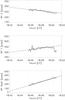 |
Fig. 6 Determination of the single wavefront RP position. Upper panel: X coordinate; middle panel: Y coordinate; lower panel: radii of the extrapolated circles. The dashed lines correspond to the linear fits. |
 |
Fig. 7 Location of the RPs: Q0 corresponds to the single wavefront; Q1, Q2, and Q3 correspond to the earliest wavefronts F1, F2, and F3. The sizes of the crosses indicate the measured error. SE indicates the small-scale ejectum origin. The FoV is 800″ × 600″. |
Determining the earliest wavefront RPs
Figure 7 shows the earliest wavefronts, i.e., the three small circular shaped fronts denoted as F1,F2, and F3. They appear sequentially in time and in ascending order. Their presence suggests either anisotropies in the local medium or the existence of more than one RP or propagating disturbance (Muhr et al. 2010). We determined the RP for each Fi to analyze them separately. We applied Procedure 1 to 27 HASTA images in the time range 18:43:26 − 18:45:36 UT for F1, 14 HASTA images in the time range 18:44:31 − 18:45:36 UT for F2 and 8 HASTA images in the time range 18:45:01 − 18:45:36 UT for F3. As in the single RP case, we find an increasing radius with time and a displacement of the RP coordinates, although the curves are more irregular. The chi-square test of the linear fits for F1 and F2 gives poor confidence.
In the same way as for the single wavefront, we obtained the RP coordinates of each earliest wavefront. The x,y linear fit, computed at the first appearance time, yielded the RP locations: Q1 = (254.7 ± 4.8,402.8 ± 14.2),Q2 = (307.7 ± 4.9,385.8 ± 11.3), and Q3 = (287.7 ± 2.9,344.5 ± 0.7). The positions of the RPs Q1,Q2, and Q3 are also shown in Fig. 7. They are approximately situated in the segment formed by F1,F2,F3 and the single RP Q0.
Procedure 2: determining chromospheric distances. We measured the chromospheric distances d traveled by the Moreton wave from the RP Q0 to a point P located over each wavefront, along great circles passing through these two points, obtained similarly to the previously described Procedure 1.
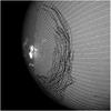 |
Fig. 8 Track of the polygonal lines or Moreton wavefronts are denoted in black; the 41 great circles passing through Q0 are denoted in white; they are equispaced by five degrees counterclockwise starting from P0. The FoV is ≈1400″ × 1400″. |
Figure 8 shows in black some of the polygonal lines representing the Moreton wavefronts, which are crossed by 41 great circles, plotted in white, covering the southwest region. These great circles were traced between Q0 = (269,422) and 41 points, Pj, obtained by counterclockwise rotating the arbitrary point P0 = (265,336), (S09.4E61.9) on the axis OQ0, 5 degrees each time. The point P0 is located 235.8° measured clockwise from the meridian passing through Q0. The wavefront positions in each HASTA image are established as the intersections of the polygonal lines representing the Moreton wavefront and the great circles j, i.e., defining K(t,j) values, j covering the 41 great circles, and t covering 65 polygonal lines. Note that the great circle 14 passes through the SF.
Figure 9 shows (solid line) the average chromospheric distance ⟨ d ⟩ of the 41 great circles, measured from the RP Q0, as a function of time in the range 18:45:40–18:51:05 UT. The vertical bars correspond to a curve dispersion of 1-sigma uncertainty. The average was calculated as ⟨ d ⟩ = Σidi/41, where di,i = 1 − 41 is the chromospheric distance measured along the i great circle defined previously. Note the smooth behavior of the initial trend and the later increase of the scatter, due to the vanishing and broadening of the wavefronts. The curve shows an initial quadratic trend in the interval 18:45:40–18:49:21 UT followed by a more linear one, after t = 18:49:21 UT. We determined the boundary between these two parts by selecting from several curve points those that minimize the errors in the quadratic fit. The time interval 18:45:41–18:49:21 UT was identified as the best fit for the quadratic curve. The dashed lines A and B in Fig. 9 correspond to two quadratic fits of the curve ⟨ d ⟩ .A is the fit for the initial quadratic interval and B is the fit considering the full set of single wavefronts. Curve C is a linear fit using the last part of curve ⟨ d ⟩, after t = 18:49:21 UT.
Curve D is a power-law fit on the complete set of single wavefronts. The power-law is  (1)where δ is the power-law exponent, c1,c2 are constants, and the initial time is ti = 18:42:00 UT. The plotted curve D has the exponent δ = 0.578627, constants c1 = 15.287, and c2 = −108.609. Figure 9 also shows the earliest wavefront chromospheric distances ⟨ d ⟩ in the time lapse: 18:43:26–18:45:40 UT. For simplicity, the distances were calculated from RP Q0. The RPs Q1, Q2, Q3 are almost aligned between F1, F2, F3 and Q0 (see Fig. 7). Note the fine concordance of the whole trend in Fig. 9, i.e., the earliest wavefronts and the single one seem to be generated simultaneously (same onset time) at a common location coincident with Q0. However, F1 has a different initial evolution that seems to deviate from the overall kinematic curve, and there is a minor misalignment at the beginning of F2.
 |
Fig. 9 Solid line: 2D averaged chromospheric distance ⟨ d ⟩ from Q0 with a 1-sigma dispersion value. Earliest wavefronts F1,F2,F3 before t = 18:45:40 UT.A: partial quadratic fit. B: total quadratic fit. C: partial linear fit. D: power-law fit. |
5. 2D kinematics of the Moreton wave event
We inferred the Moreton wavefront speed and acceleration from the linear, the quadratic, and the power-law curves fitted to the segments shown in Fig. 9 instead of using the derivative technique (see Warmuth et al. 2004a,b; Temmer et al. 2009; Muhr et al. 2005b, 2010).
We estimated the acceleration for the quadratic fits assuming a constant value and a rectilinear motion:  (2)For the power-law fit, the instantaneous modulus of acceleration is obtained as
  (3)We divided the average curve ⟨ d ⟩ into two segments: an initial quadratic trend (curve A) followed by a linear one (curve C), as indicated previously. Curves B and D correspond to the quadratic fit and the power-law fit of the full single wavefront set, respectively. Table 1 lists the calculated kinematic parameters for curves A, B, C, and D. The values listed are the onset time (t0), the accelerations a0, a1 calculated at the onset time and at the selected initial time of the single wavefront (t = 18:45:41 UT), and the instantaneous speeds s0, s1, and s2. The speed si corresponds to 1) the onset time; 2) the selected initial time of the single wavefront (t = 18:45:41 UT); 3) the completion time of the single wavefront (t = 18:49:21 UT). For the constant acceleration or the constant speed case, only a0 or s0 (curve C) is given. The acceleration and speed values obtained from curve A are similar to the highest values obtained by Warmuth et al. (2004a) when analyzing a sample of twelve Moreton events. The B and C curve values are comparable to the mean values found by Warmuth et al. (2004a). The results of these authors agree with the power-law fit of curve D obtained by our calculations. We obtained higher speed and acceleration values compared to the results obtained by Balasubramaniam et al. (2010) for the same Moreton wave event.
2D Kinematic parameters and onset times obtained from curves A, B, C, and D.
6. 2D analysis of the filament winking
The NF and SF filaments together with Q0 display a circular sector angle of ~156° (see Fig. 2a). We analyzed the winking of the NF and SF to determine their activation times and their possible correlation with the Moreton wavefront passage (Smith & Harvey 1971; Okamoto et al. 2004; Eto et al. 2002; Gilbert et al. 2008).
Moreton waves can cause the eruption of filaments in some cases. On December 6, 2006 the filaments exhibit a high intensity oscillation, i.e., both disappear completely in the Hα images and the winking can be attributed to the motion of the filament structure that shifts it out of the observed Hα bandpass (Balasubramaniam et al. 2007). As stated by Gilbert et al. (2008), the SF shows a mixture of transverse and perpendicular motion with respect to the filament spine, while the NF exhibits a less dynamic response, probably only oscillating in the plane of the sky. We obtained the light curves of three points over each filament (at the center and at both ends) and considered the activation time of a point to be the time when the point blinks, i.e., the time value where the rising light curve reaches half of its maximum value (see Fig. 10).
Figure 11 shows the scene of the wavefronts evolution on the x − y plane view centered at Q0. It provides a clearer view of the relative position of the filament points and the Moreton wavefronts with respect to the RPs. The locations of the earliest wavefronts and the small-scale ejectum are also shown.
Southern filament: the SF is situated at (S50 E11), with an average distance of 562.6 pixels (820 Mm) from the AR. It is oriented northeast-southwest, nearly parallel to the Moreton wave propagation direction and has a length of ⋍0.2 R⊙. The light curves positions are 1) PL = (641,149) for the left end; 2) PC = (681,144) for the center; and 3) PR = (719,131) for the right end (see Fig. 11). The activation times obtained are tL = 18:55:11 UT, tC = 18:55:51 UT, and tR = 18:58:11 UT. Figure 10 (left panel) shows the PL light curve.
Northern filament: the NF is sigmoid-shaped, oriented obliquely to the Moreton wave propagation direction. It is situated at (N38 E61), with an average distance of 317.5 pixels (460 Mm) from the AR. Its size is similar to that of the SF. The light curve positions are 1) PT = (250,743) for the top end, 2) PC = (260,717) for the center, and 3) PB = (270,694) for the bottom end (see Fig. 11). The activation times obtained are tT = 18:51:06 UT, tC = 18:50:41 UT, and tB = 18:48:56 UT. The NF light curve exhibits an oscillatory pattern, as can be seen for PT in Fig. 10, right panel.
We computed the chromospheric distances between the RP Q0 to the NF and to the SF previously selected points with the aim to obtain the spatio-temporal correlation of the filament activations with the Moreton wave passage. Figure 12 shows the average chromospheric distance ⟨ d ⟩ traveled by the Moreton wavefronts jointly with the filament activation points, all of them measured from Q0. The solid gray lines represent the minimum and maximum values of d. Curves A, B, C, and D were described in Sect. 5 (see Fig. 9). The three NF activation points are coincident with the visible time range of the Moreton wave event, but the wave is not visible at the location of the NF. In contrast, the SF points are activated between 3 − 6 min later than the last measured wavefront, although they are located in the zone of maximum visibility of the wave.
Figure 12 shows that the positions of the filament activation points are all seen above the curve ⟨ d ⟩ except for the NF center point. The top and bottom NF points fall within the measured error range. The extrapolation of the linear fit C for the SF (last part of curve ⟨ d ⟩) gives the closest curve to the three activation points, but the curve is separated from them by ≈100 Mm. The SF falls in the region where the Moreton wavefront seems distorted (see Fig. 11), directed toward great circle number 14. We superimposed curve d, measured along this great circle, indicated as GCSF. The straight line denoted CSF is a linear fit over curve GCSF in the time range 18:49:21–18:51:05 UT (linear trend of ⟨ d ⟩), which yields a fine coincidence with the three SF activation points. Table 1 also lists the kinematic parameters of curve CSF. We additionally indicate over the x-axis in Fig. 12 the measured times of the features that are apparently related to the ignition time of the Moreton wave event, i.e., the GOES corresponding time to half the derivative rising slope (t = 18:43:00 UT), the time corresponding to half the rising slope of the Zone 1 flare light curve (t = 18:42:45 UT) and the small-scale ejectum activation time (t = 18:42:20 UT), described in Sect. 8 of this paper.
 |
Fig. 10 2D filament light curves: activation times for SF (left) (PL = (641,149)) and NF (right) (PT = (250,743)). |
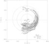 |
Fig. 11 Plane view x − y of chromospheric distances ⟨ d ⟩ centered at Q0. The dashed curves are three circles fitted to the wavefronts. NF and SF indicate the measured points of the filaments. F1, F2, and F3 indicate the earliest wavefronts. SE is the small-scale ejectum initial location. Q1, Q2, and Q3 indicate the earliest wavefront RPs. |
 |
Fig. 12 2D Space and time location for all features. Linear and quadratic fits of the coronal distance ⟨ d ⟩, averaged over the great circles corresponding to P1 − P40 related to Q0. |
 |
Fig. 13 Sequence showing the evolution of the small-scale ejectum in the TRACE images (black arrows). The FoV is ≈95″ × 175″, which is indicated in the HASTA image of Fig. 5 with a white rectangle. |
7. The flaring region seen by TRACE
TRACE images cover the full flare event with a temporal cadence of 2 s. The 160 nm UV passband filter shows atmospheric emission in the temperature range of ≈(5 × 10³ − 105) K. Since from these images it is not possible to distinguish wavefront features as in the Hα Moreton ones, we measured other dynamic characteristics to analyze their relation with the Moreton wave event.
The more relevant feature is a small-scale ejectum at the west side of the flaring region, which appears close in time with the ignition of the flare (Balasubramaniam et al. 2010). The small-scale ejectum is able to produce coronal shocks (Warmuth 2007; Pohjolainen et al. 2008; Temmer et al. 2009).
Accordingly, we measured the 2D evolution of this TRACE feature by using Procedure 2, as done with the Moreton wavefronts, i.e., first enhancing the images with the running difference technique, then identifying wavefront points and calculating their positions by intersecting great circles with polygonal lines traced over them.
The evolution of the small-scale ejectum starts at t = 18:42:20 UT and lasts ≃1 min. It has an apparent shape of a rising magnetic loop, which would indicate the eruption of a narrow filament as noted by Balasubramaniam et al. (2010). Figure 13 shows with black arrows the TRACE location of the bright plasmoid for different times, moving from northwest to southeast. The initial position of the ejectum is (234,414); (N00.7 E63.5) and is indicated as SE with a dark circle in Fig. 7. Figure 14 shows the distance traveled by the small-scale ejectum in evolution superimposed with a second-degree polynomial curve fit. We estimated a constant acceleration of a ≃ 33.8 km s-2 by using the equation of rectilinear motion with uniform acceleration. We obtained the ascending speed and height from the projected coordinate (x,y) assuming that the small-scale ejectum travels perpendicularly to the solar surface. The angle used to make calculations is the angle between the tangent plane to the sun surface at the point QSE and the plane of view, i.e., ≃63.4°. This allowed us to estimate a constant acceleration of ≃37.3 km s-2 and a final speed of ~2160 km s-1, at t = 18:43:20 UT (at the end of its visibility). By assuming that the event started its motion close to the solar surface, it is at this time that the plasmoid reaches a height of 60 Mm. We measured a radius of R ≃ 1 Mm for the plasmoid at the beginning of its evolution. Later it expanded, reaching almost R ≃ 5 Mm at t = 18:43:00 UT. Following Temmer et al. (2009), it can be argued that the small-scale ejectum is capable of producing shock waves in the solar corona.
 |
Fig. 14 2D Displacement of the small-scale ejectum as a function of time. |
 |
Fig. 15 Solid line: 2D averaged chromospheric distance ⟨ d ⟩ measured from SE together with dispersion bars. Earliest wavefronts F1, F2, and F3 plotted at t = 18:45:40 UT (indicated with a vertical line). The single wavefronts are plotted after t. Curves A, and B: partial and total single wavefronts quadratic fits. Curve C: linear single wavefronts fit. D: power-law single wavefront fit. Curves U and V: quadratic and linear fits for the earliest wavefront F1. |
8. The RP located at the origin of the small-scale ejectum
We took RP as the initial position of the ejectum SE by assuming hypothesis H3, assuming moreover that the whole Moreton event, – or part of it –, is generated by the small-scale ejectum (Warmuth et al. 2007). We measured the chromospheric distances from SE to the Moreton wavefronts and obtained the kinematic curve shown in Fig. 15. If we compare the kinematic curve of Fig. 9 with that of Fig. 15, this last shows a larger scatter of data, a misalignment of the earliest wavefront curve F3, a better alignment of the earliest wavefront F2, and a differentiated kinematic curve for the earliest wavefront F1. The F1 curve has a positive acceleration and appears to be detached from the other curves. Curves U and V correspond to a quadratic and a linear fit for F1. The quadratic fit U yields an acceleration of 4.2 ± 4.4 km s-2 and the linear fit V indicates a mean speed of 597 ± 64 km s-1.
9. Discussion
HASTA data interpretation
The HASTA December 6, 2006 event of the AR10930 can be described as a typical Moreton wave phenomenon despite its global scale.
A distinctive feature of this event is the presence of irregular shapes identified as the three earliest Moreton wavefronts. They are recognized as three circular patterns that appear sequentially. They were analyzed separately to identify more than one RP or more than one propagating disturbance (Muhr et al. 2010). We used several appropriate procedures to obtained the RP locations. We measured the chromospheric distances traveled by the wave from the calculated RPs to analyze the feasibility of different triggering mechanisms.
The kinematics of the Moreton wave event
We assumed that the RP is placed at Q0 and that the wavefront propagates spherically. An unambiguously identifiable average kinematic curve, within measurement errors, adjusts the whole phenomenon, i.e., the three earliest wavefronts as well as the single wavefront. This could indicate that the perturbation consists of a single coronal propagating wave triggered by a single ignition process.
Following Warmuth (2004a), we used a quadratic and a power-law curve fit to obtain the kinematic parameters of the event. We provided only fits for the single wavefront, i.e., the time range where the disturbance is more extended angularly and apparently just one front. Because the Moreton wave seems to be slightly decelerated with time and distance, as noted by Warmuth (2004a), we performed several fits for different parts of the curve, considering an initial quadratic evolution ending in a linear trend toward the final visible stage of the perturbation. This fitting procedure resulted in curves A and C, as shown in Fig. 12. Curve A gives a correct depiction of the dynamic behavior described by ⟨ d ⟩, from the initial visibility of the disturbance to ≈7 min later, covering a distance of ≈300 Mm. The perturbation starts with a constant deceleration of ≃− 2.4 ± 1.1 km s-2, with an initial speed of ≃1463 km s-1, slowing down to ≃696 km s-1 at the final stage of the visible time range, where the evolution is almost linear (curve C). The onset time (t0 = 18:42:28 ± 38 UT), extrapolated from the quadratic curve A reaches a good agreement with the GOES time associated to half the derivative rising slope (t = 18:43 UT), the time associated to half the rising slope of the flare light curve in Zone 1 (t = 18:42:45), and the small-scale ejectum activation time (t = 18:42:20 UT). The onset time obtained is also coincident with the peak of the photospheric net Lorentz force obtained from the GONG magnetograph, as reported by Balasubramaniam et al. (2010).
Several authors (Warmuth et al. 2001; 2004b; Veronig et al. 2006; Okamoto et al. 2004; Temmer et al. 2009) agree that there is a coincidence between the beginning of the flare and the origin of the Moreton perturbation, which supports hypothesis H1. However, other authors (Narukage et al. 2002; Muhr et al. 2010) suggest that Moreton waves are generated prior to the flare ignition, which supports hypothesis H2. The onset time obtained in this paper from curve A indicates that the Moreton wave event is generated close to the flare explosive phase (Smith & Harvey 1971). The maximum intensity of the flare, measured from the TRACE light curves, occurs ≃1 min later, at t = 18:43:27 UT.
As suggested by Balasubramaniam et al. (2010), there could be a coincidence of the onset time with the CME launch (hypothesis H2) since the photospheric changes of the Lorentz force result from changes in the coronal magnetic field, which correspond to the main acceleration phase of the CME.
The power-law fit resulting in curve D (see Fig. 12) is an accurate fit of ⟨ d ⟩ for the whole evolution of the Moreton single wavefront. The extrapolated onset time (t0 = 18:42:30 ± 01 UT) agrees with the obtained value for curve A; however, the extrapolated acceleration at the onset time (a0 = −30.2 ± 0.3 km s-2) and the corresponding speed (s0 = 2121 ± 23 km s-1) are much higher than the others. As discussed by Warmuth et al. (2004a), a strong initial deceleration of the wave could be caused by the denser medium inside the AR. In the later evolution (during the visibility of the Moreton wavefront) these values could diminish and become comparable to those obtained from curves A,B.
The fitted quadratic curve B (see Fig. 12) gives a reasonable fit for ⟨ d ⟩ throughout the evolution of the disturbance but appears to be less suitable to describe the last part of the event. Its starting constant deceleration is a0 ≃ − 1.2 ± 1.1 km s-2, with an initial speed of s0 ≃ 1170 km s-1, slowing down to s2 ≃ 510 km s-1 at the end of the visibility stage. The extrapolated onset time (t0 = 18:41:48 ± 30 UT) occurs ≃40 s before the power-law case.
As stated in Warmuth et al. (2004a), the event could be more adequately characterized with a non-constant deceleration, as is in the case of the fitting by parts (curves A and C), or in the power-law fit (curve D). This would constrain the nominal onset time to be t0 ≈ 18:42:30 UT, and the initial acceleration and speed a0,s0 would be equal to or higher than those found for curve A.
The interaction Moreton wave-filaments
We measured the activation times of NF and SF to study their winking by analyzing the light curves coming from points lying over the filaments. However, the real process of interaction between the Moreton wavefront and the quiescent structure of the prominence is unknown and these values could be inaccurate. In accord with the filament light curves, the NF exhibits a kink-mode oscillation that can be attributed to the oblique impact of the Moreton wavefront over the NF (see Fig. 11). Instead, the SF is almost perpendicular to the Moreton wavefronts and oscillates along the spine. The SF has an estimated height of 0.09 R⊙ and the lower NF height is <0.01 R⊙ (Gilbert et al. 2008). In order to test the hypothesis of a single propagating disturbance we determined whether the obtained kinematic curves can approximately explain the winking of both filaments.
The SF is located in line with the more intense Moreton disturbances, but far away from the AR, therefore it was not possible to measure the passage of the wave in its surroundings. The NF, located nearer to the AR, is outside the zone where the wave can be distinguished in the Hα images. The curves B, C, and D (see Fig. 12) are concordant with the NF position and activation time, considering the error band of the measurement. This would indicate that the evolution of the wave continues with the same trend in the north direction. Instead, the SF could only be aligned by the linear fit CSF, measured along the great circle passing over it. This fact could be attributed to changes in the physical parameters of the medium found by the shock front as it travels. The same fact would produce a noncircular shape on the latest Moreton wavefront shown in Figs. 8 and 11, which suggests that the wave evolves irregularly away from the origin, particularly in the direction of the SF. Even though the Moreton wave event is visible in a quiet chromospheric region we know that the perturbation passes through a complex magnetic region, i.e., the AR10930 southwest features.
If we consider curve A, it transforms into a straight line after the initial quadratic trend. This later linear dynamic trend is consistent with the location and time activation of the SF, by considering curve CSF. Unfortunately, the image resolution is poor in the latest images and it was not possible to obtain detailed measurements that might have led to a more reliable fit. Far from the RP, as in the case of the SF (d ≃ 800 Mm), the kinematic parameters obtained by measuring the wavefronts at the chromospheric height could also be inaccurate for the coronal event because of the solar surface curvature.
The earliest wavefronts F2 and F3 appear to be well aligned with the mean single wavefront kinematic curve (quadratic fit A, B, and D shown in Fig. 12). If the misalignment of F1 at the beginning of the curve is discarded due to the high error values, it could be asserted that the Moreton wave event is a single spherical wave generated by a single RP, which activates both filaments with the wavefront passage.
The origin of the Moreton wave event
As a first approximation, it seems that the December 6, 2006 Moreton wave event is better explained by a blast-wave scenario, in which a single source, compact and expansive, causes a spherical coronal shock wave. A blast-wave could be initiated by a pressure pulse or by an impulsive 3D piston, generating a perturbation that steepens into a shock. Moreover, the pressure pulse could be generated by the flare itself (flare-ignited wave scenario, H1, Vr nak et al. 2006).
According to Temmer et al. (2009) and Pomoell et al. (2008), a Moreton wave event can also be produced by a strong and impulsive acceleration of a source acting as a temporary piston. Therefore, the scenario of a CME-induced piston mechanism (hypothesis H2) can be related to the motion of the top of a rising flux rope (Chen et al. 2002, 2005a,b) or to the motion of the two sides of the flux rope when the flanks expand (Muhr et al. 2010; Veronig et al. 2008). Temmer et al. (2009) suggested that the lateral motion of the CME flanks is the more reliable source for a Moreton event. Conversely, Narukage et al. (2008) proposed that not the CME itself but the erupting filament can act as a piston that is responsible for the Moreton wave generation. Balasubramaniam et al. (2010) argued that the December 6, 2006 Moreton wave event is a consequence of the variation of the Lorentz force applied to the photosphere and caused by a substantial change in the coronal magnetic field that had led to the main acceleration phase of a CME. The peak of this force, which occurred at t ≈ 18:42:00 UT, shows a good coincidence with the onset times obtained in this paper (see Table 1).
Because no high acceleration values are expected for the top of the CME, a lateral acceleration ≈4.5–5.5 km s-2 would account for the time and distance needed for the Moreton shock formation. Thus, Balasubramaniam et al. (2010) postulated that the eruption of the western arcade is responsible for the CME and consequently for the Moreton coronal shock.
The RP Q0 is located to the east of the western arcade, in the direction of the flaring region. This position is not coincident with any of the likely sources of the disturbance. However, this inconsistency could be attributed to inhomogeneities of the medium that distort the initial shock formation and not to a real location of its origin, i.e., the gradient in the Alfvén speed at the border of the AR could retard the shock formation toward the AR. Although there is evidence of a halo-type CME, detailed observations are not available to analyze its relation with the Moreton wave. There is also a lack of EIT observations to study related coronal transients. Therefore, the scenario of a CME-induced piston mechanism, as suggested by Balasubramaniam et al. (2010), cannot be examined in more detail.
Regarding the flare pressure pulse scenario (hypothesis H1), Balasubramaniam et al. (2010) showed that the timing of the pressure pulse during the shock formation argues against this hypothesis. Approximate calculations led to rather extreme values of speed and acceleration. Thus, the needed scale length of the pressure pulse exceeds the size of a typical flare kernel of ~10 000 km (Vrnak & Cliver 2008). From our calculations, the timing agrees with the values obtained by Balasubramaniam et al. (2010). However, we find that initial speed values faster than 1400 km s-1 and accelerations higher than − 2.4 km s-2 are, as discussed above, feasible and thus could favor the flare pressure pulse hypothesis.
Temmer et al. (2009) reproduced a Moreton wave event by simulating the piston-like accelerated expanding source with a pressure pulse and analyzed the effects of different source sizes and velocities. By referring to hypothesis H3, our measurements of the small-scale ejectum radius of ~1 − 5 Mm and acceleration of ~37 km s-2 are at least one order of magnitude smaller and faster than those considered the most probable by Temmer et al. (2009). However, the strong acceleration of the small-scale ejectum (probably produced by magnetic structuring processes during the CME) could act as a temporary piston to generate perturbations that could steepen into shocks that propagate freely, (Warmuth et al. 2004a,b). Fast accelerated small 3D piston-like ejecta are capable of generating shock waves. As noted in Vrnak & Cliver (2008), a piston driver of the blunt type, not necessarily supersonic, generates a hyperbolic-shaped shock wave at its front. Meanwhile, the distance between the shock and the driver increases with time. The track of the shocks induced by the small-scale ejecta could presumably exhibit an accelerated motion when they arrive to the chromosphere, depending on the vertical acceleration, the direction of motion, and the speed reached by the ejecta. This could indicate that the kinematic curve with a positive acceleration corresponding to the earliest wavefront F1 shown in Fig. 15 (fitted curve U) is a shock wave generated by the motion of the small-scale ejectum. This assumption could be reinforced by the location of SE in front of the earliest wavefronts F1 shown in Fig. 11. It could be argued that the ejectum is too small to produce a chromospheric trace with the characteristics of F1. Balasubramaniam et al. (2010) suggested that the eruption of the eastern arcade could generate the northern part of the wave, and could be acting as a precursor for the western arcade eruption. If this is the case, F1 is probably the imprint of this eruption.
The proximity of SE and Q0 suggests that if two waves were launched simultaneously from these points, they would be seen superimposed at a certain distance from the origin. After the temporary pistons that generate the waves finished their actions, they would show similar kinematic evolutions. Moreover the more intense flaring region (Zone 1) is located at the vicinity of SE, therefore it is possible that the flare itself generated F1. Assuming that the small-scale ejectum produced the earliest wavefront F1, is it possible that a similar mechanism in the western arcade launched the single disturbance? This would mean a rising magnetic structure faster and less massive than the CME itself. The hypothesis that the small-scale ejectum is a precursor of the main disturbance seems incorrect. The ejectum acquires a fast speed after the probable ignition of the single disturbance, as discussed above. In contrast, the onset time and the proximity of SE to Q0 suggest that the ejectum could be initiated by the main Moreton disturbance. The first emergence of the earliest wavefront F1 could be explained as a fast 3D piston generating a shock wave, which is initially faster than the single disturbance. Later the shocks would slow down and merge, forming an apparently single wavefront.
As discussed above, the different scenarios proposed in the literature (e.g. CME generated 3D piston, flare-ignited pressure pulse) could oversimplify the description. A more complex and mixed scenario might be required to explain each observational case. Not only the origin and number of blast waves is under discussion, but also there could be more than one scenario. From this analysis it could be inferred that several distinct events were launched almost simultaneously, some of which are capable of generating shock waves in the solar corona. Their ignition could be related to a drastic magnetic restructuring of the coronal medium, which would be the CME lift-off part of this process.
10. Conclusions
We conclude that the Moreton wave event observed on December 6, 2006 detected with the Hα Solar Telescope for Argentina (HASTA), is a coronal fast-shock wave of a “blast” type originated in a single source during a CME. Its onset time is concurrent with the peak of the Lorentz force applied to the photosphere measured by other authors for the same event. The event shows an overlap with the flare explosive phase and small-scale ejectum ignition. The kinematic parameters obtained, i.e., the onset time of the event (t0 ≃ 18:42:28 UT), the initial deceleration (a0 ≥ 2.4 km s-2), and the initial speed (s0 ≥ 1463 km s-1), are higher than those obtained by other authors for the same event. Simultaneously with the evolution of the shock wave, two distant filaments were activated.
The wavefronts have local irregularities that can be attributed to inhomogeneities of the coronal medium that crosses the disturbance. At the initial stages, the three earliest wavefronts, which can be regarded as a result of these irregularities, appear to be detached. However, the first of them could be considered to have a kinematic evolution different from that the others. This could occur if the origin is placed east-side of the RP, in the surroundings of the small-scale ejectum location, which could indicate a separate origin for this earliest wavefront.
Acknowledgments
We are grateful to L. Balmaceda, J. Castro, M. Schneiter, G. Stenborg and R. Torres for their comments and useful discussions.
References
- Bagalá, L. G., Bauer, O. H., Fernández Borda, R., et al. 1999, European Meeting on Solar Physics Magnetic Fields and Solar Processes, ESA SP, 448, 469 [NASA ADS] [Google Scholar]
- Balasubramaniam, K., Pevtsov, A., & Neidig, D. 2007, ApJ, 658, 1372 [NASA ADS] [CrossRef] [Google Scholar]
- Balasubramaniam, K., Cliver, E., Pevtsov, A., et al. 2010, ApJ, 723, 587 [NASA ADS] [CrossRef] [Google Scholar]
- Brueckner, G., Howard, R., Koomen, M., et al. 1995, Sol. Phys., 162, 357 [NASA ADS] [CrossRef] [Google Scholar]
- Chen, P. F., Wu, S. T., Shibata, K., & Fang, C. 2002, ApJ, 572, L99 [NASA ADS] [CrossRef] [Google Scholar]
- Chen, P. F., Ding, M. D., & Fang, C. 2005a, Sp. Sc. Rev., 121, 201 [Google Scholar]
- Chen, P. F., Fang, C., & Shibata, K. 2005b, ApJ, 622, 1202 [Google Scholar]
- Eto, S., Isobe, H., Narukage, N., et al. 2002, PASJ, 54, 481 [NASA ADS] [CrossRef] [Google Scholar]
- Gilbert, H. R., Daou, A. G., Young, D., Tripathi, D., & Alexander, D. 2008, ApJ, 685, 629 [NASA ADS] [CrossRef] [Google Scholar]
- Handy, B. N., Acton, L. W., Kankelborg, C. C., et al. 1999, Sol. Phys., 187, 229 [NASA ADS] [CrossRef] [Google Scholar]
- Moreton, G. E., & Ramsey, H. E. 1960, PASP, 72, 357 [Google Scholar]
- Muhr, N., Vršnak, B., Temmer, M., Veronig, A. M., & Magdalenić, J. 2010, ApJ, 708, 1639 [Google Scholar]
- Narukage, N., Ishii, T., Nagata, S., et al. 2008, ApJ, 684, L45 [Google Scholar]
- Narukage, N., Hudson, H. S., Morimoto, T., et al. 2010, ApJ, 572, L109 [Google Scholar]
- Okamoto, T., Nakai, H., Keiyama, A., et al. 2004, ApJ., 608, 1124 [NASA ADS] [CrossRef] [Google Scholar]
- Pohjolainen, S., Hori, K., & Sakurai, T. 2008, Sol. Phys., 253, 291 [NASA ADS] [CrossRef] [Google Scholar]
- Pomoell, J., Vainio, R., & Kissmann, R. 2008, Sol. Phys., 253, 249 [NASA ADS] [CrossRef] [Google Scholar]
- Smith, S., & Harvey, K. 1971, Physics of the Solar Corona, ed. C. J. Macris (Dordrecht: Reidel), 156 [Google Scholar]
- Temmer, M., Vršnak, B., Žic, T., & Veronig, A. M. 2009, ApJ, 702, 1343 [NASA ADS] [CrossRef] [Google Scholar]
- Uchida, Y. 1968, Sol. Phys., 4, 30 [NASA ADS] [CrossRef] [Google Scholar]
- Uchida, Y., Altschuler, M. D., & Newkirk, G. 1973, Sol. Phys., 28, 495 [Google Scholar]
- Veronig, A., Temmer, M., Vršnak, B., & Thalmann, J. 2006, ApJ, 647, 1466 [NASA ADS] [CrossRef] [EDP Sciences] [Google Scholar]
- Veronig, A., Temmer, M., & Vršnak, B. 2008, ApJ, 681, 113 [Google Scholar]
- Vršnak, B., Warmuth, A., Temmer, M., et al. 2006, A&A, 448, 739 [Google Scholar]
- Vršnak, B., & Cliver, E. 2008, Sol. Phys., 253, 215 [NASA ADS] [CrossRef] [Google Scholar]
- Warmuth, A., Vršnak, B., Aurass, H., & Hanslmeier, A. 2001, ApJ, 560, L105 [Google Scholar]
- Warmuth, A., Vršnak, B., Magdalenie, J., Hanslmeier, A., & Otruba, W. 2004a, A&A, 418, 1101 [NASA ADS] [CrossRef] [EDP Sciences] [Google Scholar]
- Warmuth, A., Vršnak, B., Magdalenie, J., Hanslmeier, A., & Otruba, W. 2004b, A&A, 418, 1117 [NASA ADS] [CrossRef] [EDP Sciences] [Google Scholar]
- Warmuth, A. 2007, The High Energy Solar Corona: Waves, Eruptions, Particles, eds. K.-L. Klein, & A. L. MacKinnon (Springer) Lect. Notes Phys., 725, 107 [Google Scholar]
All Tables
All Figures
|
Fig. 1 GOES11: integrated X-ray flux, 1 − min averaged. The shaded area corresponds to the visibility range of the Moreton wave event. XL: (1–8 Å), XS: (0.5–3 Å). |
| In the text | |
|
Fig. 2 Left: HASTA observation of NOAA AR10930, northern (NF) and southern filaments (SF). Right: MDI photospheric magnetic field distribution (white/black corresponding to +/− polarity). |
| In the text | |
|
Fig. 3 HASTA evolution of the Moreton wave event. The images were treated to enhance the wave. |
| In the text | |
|
Fig. 4 NOAA AR10930 light curves. Upper panel: whole region; upper middle panel: zone 1; lower middle panel: zone 2; lower panel: zone 3. |
| In the text | |
|
Fig. 5 HASTA view of the NOAA AR10930 at t = 18:45:35 UT. The dark rectangles indicate the three HASTA zones. The FoV is 232″ × 260″ centered at P = (248,420), which corresponds to the region denoted in Fig. 2, left panel. The white rectangle indicates the TRACE region shown in Fig. 13. |
| In the text | |
|
Fig. 6 Determination of the single wavefront RP position. Upper panel: X coordinate; middle panel: Y coordinate; lower panel: radii of the extrapolated circles. The dashed lines correspond to the linear fits. |
| In the text | |
|
Fig. 7 Location of the RPs: Q0 corresponds to the single wavefront; Q1, Q2, and Q3 correspond to the earliest wavefronts F1, F2, and F3. The sizes of the crosses indicate the measured error. SE indicates the small-scale ejectum origin. The FoV is 800″ × 600″. |
| In the text | |
|
Fig. 8 Track of the polygonal lines or Moreton wavefronts are denoted in black; the 41 great circles passing through Q0 are denoted in white; they are equispaced by five degrees counterclockwise starting from P0. The FoV is ≈1400″ × 1400″. |
| In the text | |
|
Fig. 9 Solid line: 2D averaged chromospheric distance ⟨ d ⟩ from Q0 with a 1-sigma dispersion value. Earliest wavefronts F1,F2,F3 before t = 18:45:40 UT.A: partial quadratic fit. B: total quadratic fit. C: partial linear fit. D: power-law fit. |
| In the text | |
|
Fig. 10 2D filament light curves: activation times for SF (left) (PL = (641,149)) and NF (right) (PT = (250,743)). |
| In the text | |
|
Fig. 11 Plane view x − y of chromospheric distances ⟨ d ⟩ centered at Q0. The dashed curves are three circles fitted to the wavefronts. NF and SF indicate the measured points of the filaments. F1, F2, and F3 indicate the earliest wavefronts. SE is the small-scale ejectum initial location. Q1, Q2, and Q3 indicate the earliest wavefront RPs. |
| In the text | |
|
Fig. 12 2D Space and time location for all features. Linear and quadratic fits of the coronal distance ⟨ d ⟩, averaged over the great circles corresponding to P1 − P40 related to Q0. |
| In the text | |
|
Fig. 13 Sequence showing the evolution of the small-scale ejectum in the TRACE images (black arrows). The FoV is ≈95″ × 175″, which is indicated in the HASTA image of Fig. 5 with a white rectangle. |
| In the text | |
|
Fig. 14 2D Displacement of the small-scale ejectum as a function of time. |
| In the text | |
|
Fig. 15 Solid line: 2D averaged chromospheric distance ⟨ d ⟩ measured from SE together with dispersion bars. Earliest wavefronts F1, F2, and F3 plotted at t = 18:45:40 UT (indicated with a vertical line). The single wavefronts are plotted after t. Curves A, and B: partial and total single wavefronts quadratic fits. Curve C: linear single wavefronts fit. D: power-law single wavefront fit. Curves U and V: quadratic and linear fits for the earliest wavefront F1. |
| In the text | |
Current usage metrics show cumulative count of Article Views (full-text article views including HTML views, PDF and ePub downloads, according to the available data) and Abstracts Views on Vision4Press platform.
Data correspond to usage on the plateform after 2015. The current usage metrics is available 48-96 hours after online publication and is updated daily on week days.
Initial download of the metrics may take a while.