| Issue |
A&A
Volume 551, March 2013
|
|
|---|---|---|
| Article Number | A134 | |
| Number of page(s) | 9 | |
| Section | Interstellar and circumstellar matter | |
| DOI | https://doi.org/10.1051/0004-6361/201220904 | |
| Published online | 06 March 2013 | |
The twofold debris disk around HD 113766 A⋆
Warm and cold dust as seen with VLTI/MIDI and Herschel/PACS
1 Max Planck Institut für Astronomie, Königstuhl 17, 69117 Heidelberg, Germany
e-mail: This email address is being protected from spambots. You need JavaScript enabled to view it.
2 UJF-Grenoble 1/CNRS-INSU, Institut de Planétologie et d’Astrophysique de Grenoble (IPAG), UMR 5274, Grenoble, France
3 Leiden Observatory, Leiden University, PO Box 9513, 2300 RA Leiden, The Netherlands
4 Astronomy Department, University of Texas at Austin, 1 University Station C1400, Austin, TX 78712-0259, USA
5 Département d’Astrophysique, Géophysique et Océanographie, Université de Liège, 17 Allée du Six Août, 4000 Sart Tilman, Belgium
6 University Heidelberg, Kirchhoff-Institut für Physik, 69120 Heidelberg, Germany
Received: 13 December 2012
Accepted: 22 January 2013
Abstract
Context. Warm debris disks are a sub-sample of the large population of debris disks, and display excess emission in the mid-infrared. Around solar-type stars, very few objects (~2% of all debris disks) show emission features in mid-IR spectroscopic observations that are attributed to small, warm silicate dust grains. The origin of this warm dust could be explained either by a recent catastrophic collision between several bodies or by transport from an outer belt similar to the Kuiper belt in the solar system.
Aims. We present and analyze new far-IR Herschel/PACS photometric observations, supplemented by new and archival ground-based data in the mid-IR (VLTI/MIDI and VLT/VISIR), for one of these rare systems: the 10–16 Myr old debris disk around HD 113766 A. We improve an existing model to account for these new observations.
Methods. We implemented the contribution of an outer planetesimal belt in the Debra code, and successfully used it to model the spectral energy distribution (SED) as well as complementary observations, notably MIDI data. We better constrain the spatial distribution of the dust and its composition.
Results. We underline the limitations of SED modeling and the need for spatially resolved observations. We improve existing models and increase our understanding of the disk around HD 113766 A. We find that the system is best described by an inner disk located within the first AU, well constrained by the MIDI data, and an outer disk located between 9–13 AU. In the inner dust belt, our previous finding of Fe-rich crystalline olivine grains still holds. We do not observe time variability of the emission features over at least an eight-year time span in an environment subjected to strong radiation pressure.
Conclusions. The time stability of the emission features indicates that μm-sized dust grains are constantly replenished from the same reservoir, with a possible depletion of sub- μm-sized grains. We suggest that the emission features may arise from multi-composition aggregates. We discuss possible scenarios concerning the origin of the warm dust observed around HD 113766 A. The compactness of the innermost regions as probed by the MIDI visibilities and the dust composition suggest that we are witnessing the results of (at least) one collision between partially differentiated bodies, in an environment possibly rendered unstable by terrestrial planetary formation.
Key words: stars: individual: HD 113766 A / zodiacal dust / circumstellar matter / infrared: stars / techniques: spectroscopic / techniques: high angular resolution
Based on Herschel observations, OBSIDs: 1342227026, 1342227027, 1342237934, and 1342237935. Herschel is an ESA space observatory with science instruments provided by European-led Principal Investigator consortia and with important participation from NASA. Based on VISIR observations collected at the VLT (European Southern Observatory, Paranal, Chile) with program 089.C-0322(A).
© ESO, 2013
1. Introduction
Debris disks are byproducts of the planet formation process once the massive, gas-rich circumstellar disk has dissipated. After the gas disks are lost, planetary systems including asteroids and comets may remain and evolve through gravitational interactions. The presence of dust, which originates from the collisions or evaporation of these bodies, translates into a mid- to far-infrared (IR) excess, as demonstrated for the first time for Vega (Aumann et al. 1984) using the Infrared Astronomical Satellite. Departure from photospheric emission at these wavelengths is the consequence of thermal emission arising from dust grains heated by the stellar radiation. Several hundred stars are now known to harbor such excess emission (e.g., Chen et al. 2006). Our understanding of their nature has progressed during the past decades, both observationally and theoretically (see Wyatt 2008 and Krivov 2010 for recent reviews). In most cases, these systems compare very well with the Kuiper belt observed in our solar system (e.g., Carpenter et al. 2009; Liseau et al. 2010; Löhne et al. 2012), where excess emission is detected in the far-IR. Several studies made use of high angular resolution instruments to detect hot exozodiacal dust around well-known debris disks (e.g., Fomalhaut and Vega, see Absil et al. 2009; Defrère et al. 2011, respectively). In such cases, the near-IR excess is relatively small (~1%) and departure from photospheric emission only becomes significant at mid- or far-IR wavelengths. A small sample of the debris disk population is referred to as “warm debris disks” (e.g., Moór et al. 2009), where emission in excess is significant in the mid-IR, suggesting the presence of warm dust grains close to the star. Within this class of warm debris disks, a few objects are of particular interest since they also display emission features in mid-IR spectroscopic observations. These emission features are associated with (sub-) μm-sized dust grains that are warm enough to contribute significantly in the mid-IR (see Henning 2010 for a review on optical properties of silicate dust).
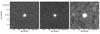 |
Fig. 1 Herschel/PACS observations at 70, 100, and 160 μm (left to right). |
These warm debris disks with emission features around solar-type stars are rare (~2% of all debris disks, Bryden et al. 2006; Chen et al. 2006). As discussed in Wyatt (2008), the abnormal brightness of these debris disks cannot be solely explained by a steady state collisional evolution. If it was, the collisional lifetime of the parent bodies responsible for the dust production, and hence the infrared luminosity, would be too short compared to the age of the host star. Consequently, two scenarios are possible, either a recent catastrophic collision between two planetesimals, or an outer belt feeding the inner regions, for instance via scattering of bodies by one ore more planets (Bonsor et al. 2012), or in a similar scenario to the late heavy bombardment phase, that happened in the solar system (Gomes et al. 2005). The overall scarcity of the “warm debris disk” phenomenon would suggest a relatively low probability for such events to happen and produce enough dust to be detected. Thorough studies of such objects can therefore improve our understanding of the final steps of planetary formation, and can provide important clues to the origin of zodiacal dust or Kuiper-belt dust in our solar system.
The binary system HD 113766 is one of these rare warm debris disks that show prominent emission features in the mid-IR. The system is a binary of two almost identical stars with spectral types F3/F5, with a projected separation of 1.3′′ (~160 AU at d⋆ = 123 pc, van Leeuwen 2007), the dust being located around the primary HD 113766 A (L⋆ = 4.4 L⊙, Lisse et al. 2008). The Spitzer/IRS spectrum of the 10–16 Myr old debris disk was first studied by Lisse et al. (2008). In Olofsson et al. (2012) we presented a first model to reproduce the Spitzer/IRS spectrum of this source. In the following we present new Herschel/PACS photometric observations at 70, 100, and 160 μm, supplemented by archival VLTI/MIDI interferometric measurements as well as (new and archival) VLT/VISIR observations in the N- and Q-bands. In Sect. 2 we describe the observations and data processing; in Sect. 3 we present our model and results. We discuss the implications of our findings in Sect. 4 before concluding.
2. Observations and data processing
2.1. Herschel/PACS observations
We observed HD 113766 A with the PACS photometer (Poglitsch et al. 2010) onboard Herschel (Pilbratt et al. 2010). The dataset consists of four PACS mini-scan maps (program “OT1_jolofsso_1”), two in the blue filter (70 μm, OBSIDs 1342227026 and 1342227027), and two in the green filter (100 μm, OBSIDs 1342237934 and 1342237935). The observing duration was 220 × 2 s in the blue filter and 670 × 2 s in the green filter. When observing with PACS with the blue camera (blue or green filters, at 70 and 100 μm, respectively), data is also simultaneously acquired with the red camera (160 μm). We therefore combined the four mini-scan maps in the red filter to obtain the photometry at 160 μm.
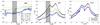 |
Fig. 2 VLTI/MIDI visibilities and correlated fluxes for HD 113766 A (left and middle panels, respectively). The baselines used and their lengths are reported in the caption of the left panel. Right panel shows the VISIR N-band spectrum at different epochs (2009 and 2012, in thick red and thin blue, respectively). The Spitzer/IRS spectrum is shown in open black circles in the middle and right panels. |
The data were processed using the Herschel interactive processing environment (HIPE, version 10.0.667), using standard scripts that include bad pixel flagging, detection and correction for glitches and HighPass filtering in order to remove the 1/f noise (see Poglitsch et al. 2010 for more details). We discarded the first column of each detector sub-array in order to eliminate electronic crosstalk. Finally, we processed the data with different HighPass filter widths to test the robustness of the data reduction. The different values are tabulated in Table 1 (Col. HP).
The aperture photometry in all three filters was extracted within HIPE from the combined maps. The aperture radii are set at 10′′ for the blue and green filters and 20′′ for the red filter. The final flux values do not depend on the aperture sizes since an aperture correction is performed to compensate for flux loss outside of the aperture. This correction is based on a calibrated encircled energy fraction parametrisation contained in the calibration data that is included in HIPE. In order to estimate the noise level and thus the quality of the detection in all filters, we randomly placed apertures within a distance of 100, 75, and 50 pixels (for blue, green, and red filters, respectively) from the central pixel. Doing so, we avoided borders of maps that are noisier due to a smaller detector coverage, and are therefore not representative of the noise close to the source. We extracted the photometry for all of these apertures and then fitted a Gaussian profile to the flux distribution histogram to estimate the σ uncertainty from the width of the Gaussian. Overall, these uncertainties are consistent with predictions from the HerschelSpot1 software. Figure 1 show the PACS images at 70, 100, and 160 μm (left to right, respectively), where the source is clearly detected at all three wavelengths. Table 1 summarizes the final results of the data processing, with pixel sizes for the three filters, aperture corrected fluxes for the different HighPass filter widths, and estimated 1σ uncertainties in units of mJy. The fluxes used in the analysis are the averages of those reported in Table 1. For all three filters, the photometric values are almost identical for the different HighPass filter widths within the uncertainties. One should notice that the measured 70 μm flux is consistent with the Mips observations reported by Chen et al. (2011, F70 = 390 ± 11.
Final products of Herschel/PACS data processing.
2.2. Complementary observations
In addition to the far-IR observations, we included the Spitzer/IRS spectrum of HD 113766 A (between 5 and 35 μm) in the analysis (see Olofsson et al. 2012 for details on the data processing). We supplemented these data with VLT/VISIR observations (our program and data published in Smith et al. 2012) and VLTI/MIDI interferometric measurements (Smith et al. 2012).
On the night of 2012-Apr-21, HD 113766 A was observed with the VLT/VISIR instrument (program 089.C-0322(A)) in the N-band. We defined four spectral windows, centered at 8.8 μm (8.0 ≤ λ ≤ 9.6 μm), 9.8 μm (9.0 ≤ λ ≤ 10.6 μm), 11.4 μm (10.4 ≤ λ ≤ 12.5 μm), and 12.4 μm (11.4 ≤ λ ≤ 13.5 μm) in low resolution mode (R ~ 350 at 10 μm). We additionally retrieved the spectroscopic observations presented and analyzed in Smith et al. (2012). These observations were also performed in low resolution mode on the night of the 2009-May-11 for two spectral windows centered at 8.8 and 11.4 μm (program 083.C-0775(E)). Both datasets were processed using standard scripts provided within the ESO Gasgano software2. The right panel of Fig. 2 shows the IRS and VISIR spectra obtained in 2004, 2009, and 2012 (open black circles, thick red, and thin blue lines, respectively). One should note that both VISIR spectra, taken almost three years apart agree surprisingly well. However, the spectrum obtained in our program in the 9.8 μm spectral window displays an offset of about 10% higher in flux. Such “stiching” problems are not unusual, but the exact causes are not clear. We checked the atmospheric conditions during our observing program: the seeing and atmospheric pressures appear to be constant over the run. Besides the 9.8 μm band offset, both VISIR spectra show a deficit of flux of about 30% compared to the IRS spectrum. Smith et al. (2012) already discussed in detail these differences (e.g., spatially extended emission) and concluded these differences to be within the absolute calibration uncertainites of VISIR (see discussion in Geers et al. 2007).
The archival MIDI data presented in Smith et al. (2012) were processed using scripts dedicated to observations of faint targets with MIDI (see Burtscher et al. 2012 for more details) interfaced with the MIA+EWS software3. Table 2 summarizes the observing log for the interferometric measurements. As in Smith et al. (2012), we found that the observations performed on the night of 2007-May-30 (program 079.C-0259(F)) had a low signal to noise ratio, and we did not include them in our analysis. The calibrated visibilities and correlated fluxes for HD 113766 A are displayed in the left and middle panels of Fig. 2. The IRS spectrum is also shown for comparison to the correlated fluxes. Because of the challenge of accurately calibrating the VISIR spectra, we used the IRS spectrum to compute visibilities from the correlated fluxes. The calibrated dataset compares very well with the data reduction of Smith et al. (2012), except for one single run (083.C-0775(B), observed at 05:32:55). When calibrating these observations with their corresponding calibrator (HD 112213, observed at 05:15:45), we found a correlated flux much higher than the IRS spectrum. We constructed the transfer function based on all the calibrators observed during that night. At the time of the science observations, we found a variation of about a factor of 2 compared to the average transfer function over the rest of the night. This suggests that the observing conditions were strongly varying. We reduced these science observations with a later observation of the same calibrator (06:34:00). One can see in Fig. 2 that both visibilities and correlated fluxes are large for this run (orange dashed line) and that there is a fairly significant difference with the consecutive observations on the same night with the same baseline (06:09:53, orange dotted line). As explained in Burtscher et al. (2012), uncertainties are given by the quadratic sum of the photon noise error delivered by the MIA+EWS software and the standard deviation of the transfer function over the night of observations. Overall, the final uncertainties are dominated by the standard deviation (between 5 and 10%). For the “problematic” observing run (083.C-0775(B), time 05:32:55) the standard deviation of the transfer function over the night is closer to 25%.
We did not reduce the VLT/VISIR images analyzed in Smith et al. (2012). We instead used the full width at half maximum (FWHM) presented in their study. In none of the N- and Q-band images (λc = 11.85 and 18.72 μm, with Δλ = 2.34 and 0.88 μm, respectively) presented by the authors, was the debris disk spatially resolved compared to a reference point spread function (PSF). They fitted the azimuthally averaged surface brightness distributions with Gaussian profiles with FWHM of 0.322′′ and 0.498′′ in the N- and Q-bands, respectively. During the analysis, we will check if synthetic images convolved with such PSFs are consistent with the measurements of Smith et al. (2012). After convolving the synthetic images with the reference PSF, we will compare the surface brightness distribution to check for possible resolved emission in both bands.
3. Multi-technic, multi-wavelength modelling
As in Olofsson et al. (2012), a given debris belt is fully described by four free parameters plus a dust model: the inner and outer radii of the dust belt (rin and rout), a volume density exponent α (Σ(r) = Σ0(r/r0)α, α < 0), and an exponent p for the grain size distribution (dn(s) ∝ spds, p < 0). The Σ0 reference value is found by adjusting the total mass of the dust Mdust, which in turn is obtained by fitting the SED. The relative abundances for the different dust species are also free parameters in the modeling and are found by fitting the SED and the emission features detected in the IRS spectrum. For each set of rin, rout, α, and p, the fitting of the abundances is performed via a Levenberg-Marquardt algorithm on a linear combination of the thermal contributions of all the dust species considered. The best-fit disk model is found via a Monte-Carlo Markov chain (MCMC) exploration of the parameter space (emcee package, Foreman-Mackey et al. 2012). All the uncertainties quoted in the next sections represent the standard deviations of all the values tested during the fitting process.
In the following we will first present a model of the debris disk assuming that the dust is distributed in a single belt around the central star (referred to as model 1B for “one belt”). We will test the robustness of this model, comparable to the one presented in Olofsson et al. (2012), with respect to the new far-IR photometric observations and mid-IR interferometric measurements. The Herschel data provide new constraints on the cold counterpart of the debris disk, while the mid-IR MIDI data are more sensitive to the warmer dust and provide direct information on the geometry of the dust distribution; the interferometric observations suggest the region emitting in the N-band is compact (≲10 mas, or 1.2 AU in diameter, according to Smith et al. 2012). In contrast, our previous best-fit model described in Olofsson et al. (2012) was found to be fairly extended (rout ~ 12 AU, with a density profile with an exponent of α = −1.8). We can therefore foresee that fitting the SED and the MIDI data simultaneously will be challenging.
In order to compare our model to the MIDI and VISIR observations we updated the Debra code to produce synthetic images at different wavelengths. To do this, at a given wavelength we distribute the thermal surface brightness distribution (Fν(r), between rin and rout), assuming the disk is axisymmetric and infinitely flat. Possible inclination effects are taken into account by projecting pixels of the image onto the sky plane. However, because we assumed the disk to be infinitely flat, we chose the inclination i (0° being face-on) to be smaller than 60°. In the case of HD 113766 A this choice is supported by the analysis of Smith et al. (2012) who could successfully model the MIDI data with a circularly symmetric flux distribution (i.e., small i). As we are solely interested in the variation of the visibilities as a function of the baseline lengths, we averaged the MIDI visibilities in the spectral range 10.5 ± 0.5 μm for each MIDI baseline. We tested different values for i and the position angle (PA) of the debris disk. We tested four different values for i (0, 20, 40, and 60°) and 30 values linearly distributed between 0 and 180° for the PA (0° meaning the semi-major axis is oriented along the north-south direction).
3.1. One belt model (1B)
Best-fit results for the disk parameters for both the 1B and 2B models.
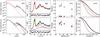 |
Fig. 3 Upper and lower panels: results for the 1B and 2B models. Left panel: SED of HD 113766 A. The IRS spectrum is in black, PACS data are shown as black open circles. For the 1B model, the final best fit is in red. For the 2B model, the final total fit is in green, the separate contributions of the inner and outer belts are in red and blue, respectively. Middle left panel: blow-up of the stellar subtracted IRS spectrum. Color coding is the same as for the left panel. Residuals (100 × [ Fν,obs − Fν,mod ] /Fν,obs) are displayed below the spectra. Middle right panel: observed and modeled MIDI visibilities as a function of the baseline (open black circles and red squares, respectively, with 1σ uncertainties). Right panel: modeled surface brightness at 10 and 20 μm (thin and thick black lines, respectively) of synthetic images convoled with 2D Gaussian with FWHM of 0.322 and 0.498′′. The 2D Gaussian with the aforementioned FWHM, assumed to be PSF representative of the images, are shown in thin and thick dashed red lines for comparison. |
At first we tried to model solely the SED, including the new PACS photometric points and the IRS spectrum. As mentioned earlier, the MIDI data suggest that the regions emitting in the N-band is compact (r ≤ 1.2 AU). Therefore, we first want to test how robust the assumption of a single dust belt is, with respect to the far-IR measurements, and to underline at the same time the limitations of such approach. We will then compare the best-fit 1B model to the interferometric data and discuss the subsequent implications on the spatial distribution of the dust. The dust properties (absorption efficiences and grain sizes) are the same as the ones described in Olofsson et al. (2012). Grain sizes for the crystalline dust grains are 0.1 ≤ s ≤ 1 μm, and for the amorphous dust grains 0.1 μm ≤ s ≤ 1 mm. The minimum and maximum values for the grain sizes are not free parameters in the modeling. This choice mostly originates from the experimental setup for the laboratory experiments that led to the extinction efficiencies of crystalline olivine grains (see Olofsson et al. 2012 for more details).
Modeling only the SED with the new far-IR observations, we now find the dust to be located between (0.4 ± 0.2) AU and (51.9 ± 25.2) AU, with a volume density exponent of α = −1.9 ± 0.3, and an exponent for the grain size distribution p = −3.0 ± 0.1. The total dust mass is 1.3 × 10⁻² M⊕. The relative abundances for the different dust species are as follows: (43.1 ± 1.4)% of amorphous silicates (with a predominance of MgFeSi2O6 and MgFeSiO4 grains, optical constant from Dorschner et al. 1995), (17.3 ± 0.7)% of Mg-rich crystalline olivine grains, (21.0 ± 0.6)% of Fe-rich crystalline olivine grains (laboratory measurements from Tamanai & Mutschke 2010 for the olivine data), (11.6 ± 0.5)% of enstatite (Jäger et al. 1998a), (0.0 + 0.8)% of β-cristobalite (Tamanai 2010), and (7.0 ± 0.6)% of amorphous carbon dust grains (Jäger et al. 1998b, mostly in the form of cellulose pyrolized at 800 °C, “cel800”). Disk parameters for the best-fit model are reported in the first line of Table 3.
Fits to the SED, the stellar subtracted IRS spectrum, MIDI data, and a comparison to the VISIR images are displayed on the upper four panels of Fig. 3 (left to right, respectively). For the SED, the IRS spectrum is shown in black, the PACS data are shown as black open circles, and the best fit is represented as a solid red line. The color coding is the same for the blow up of the fit to the IRS spectrum (second column), and residuals are shown below the fit. Residuals are computed as 100 × [ Fν,obs − Fν,mod ] /Fν,obs, where Fν,obs and Fν,mod are the observed and modeled fluxes. The third column panel shows the observed and modeled MIDI visibilities for the best-fit to the SED (uncertainties are 1σ). The right panel shows the comparison between the PSFs fitted to the VISIR observations (Smith et al. 2012) in the N- and Q-bands and the azimuthally averaged profiles of synthetic images for the final best-fit model, convolved with PSFs with FWHMs of 0.322′′ and 0.498′′, respectively, as in Smith et al. (2012).
While the best-fit model agrees well with the SED and the IRS spectrum, the observed MIDI visibilities are severely under-predicted. As discussed above, this can be explained by the relative compactness of the emitting regions probed by the interferometric data. The N-band emission in our best-fit model is too extended and therefore the modeled visibilities drop very quickly. This is also true for the VISIR observations. The modeled surface brightness profiles over-predict the observed 2D Gaussian profiles assumed to be representative of the PSFs in the N-band and even more in the Q-band (the disk was not resolved in the VISIR observations).
As a final test, we tried to include the MIDI observations in the fitting process (by summing the reduced  from the fits to the SED and MIDI data), but could not achieve any better results. Both the MIDI and the mid- to far-IR segment of the SED are under-predicted. This can be explained as a tradeoff between the compactness of the dust belt and its contribution to the far-IR. Under the assumption of a single dust belt, the fits to the SED and interferometric data are diametrically opposed. From a modeling perspective, the main conclusion of this exercise is that SED modeling can be misleading: as shown in the upper left panel of Fig. 3, we could obtain a decent fit to the SED, but this model is quickly proven wrong as soon as spatially resolved observations are available.
3.2. Two belts model (2B)
Several recent studies have shown that debris disks may contain several planetesimal belts (e.g., Morales et al. 2011, or the disk around τ Ceti, di Folco et al. 2007; Greaves et al. 2004). We have shown in Sect. 3.1 that the assumption of one single dust belt around HD 113766 A cannot account for all the available dataset. We can therefore start discussing the possibility of two, spatially separated dust belts around the central star: an inner dust belt, compact and close to the star that can reproduce the MIDI data and the near- to mid-IR flux, and a second dust belt, farther away from the star that will contribute to the emission in the far-IR. To account for an additional belt, the modification to be applied to the Debra code is straightforward, as we simply duplicated the computations done for one dust belt to the second one. A second radial grid, with different rin and rout values, with its own volume density (α) is generated, as well as the corresponding dust temperatures as the function of the grain sizes and compositions. The dust properties in the outer belt can be defined separately from the properties in the inner belt (different dust species, smin, smax, and p). Finally, the fitting to the SED is performed over the sum of the contributions of the two dust belts (returning the dust mass for each belt).
As discussed in Olofsson et al. (2012), the radiation pressure force is strong around HD 113766 A. We computed the unitless β ratio between the radiation pressure and gravitational forces for different grain sizes and dust compositions as described in Burns et al. (1979). We find that grains with sizes smaller than (4 ± 0.5) μm (depending on their compositions) are expected to be short-lived around the central star (see Sect. 4.1). However, the detection of strong emission features indicates that warm (sub-) μm-sized grains must be located close to the star to contribute to the IRS spectrum. Therefore, the dust properties (absorption efficiencies and grain sizes) of the innermost dust belt in the two-belt model (2B) are chosen to be similar to the 1B model (Sect. 3.1), regardless of the radiation pressure issue. The relative abundances are still free parameters. For the outer dust belt, we did not include such small grains. The ratio β between the radiation pressure and gravitational forces is distance-independent (both forces decreasing as r-2, their ratio no longer depends on r), while the collisional timescale is longer at greater distances (Sect. 4.1). We set the minimum grain size to smin = 4 μm for all dust species in the outer belt, as there is no observational evidence, such as emission features at long wavelengths, that would require including smaller dust grains. Because we assumed in our model that crystalline dust grains have sizes smaller than 1 μm, they are not accounted for in the outer belt (see Sect. 4.3 for further discussion). This time, for each model of the MCMC run we fitted the SED and the MIDI observations simultaneously.
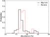 |
Fig. 4 Probability distributions from the MCMC run for model 2B, as a function of relative abundances of Mg- and Fe-rich olivine grains (solid black and dashed red, respectively). |
For the inner dust belt, we obtained a best fit to the data with dust being located between (0.6 ± 0.1) AU and (0.9 ± 0.2) AU, a density profile in α = −1.7 ± 0.3, and a grain size distribution exponent of − 3.5 ± 0.1 (consistent with the prediction for a collisional cascade p = −3.5, Dohnanyi 1969). The total dust mass is 9.0 × 10⁻⁵ M⊕. The relative abundances for the inner belt are the following: (44.5 ± 1.4)% of amorphous silicate grains (dominated by Mg2SiO4 grains, optical constant from Jäger et al. 2003), (17.0 ± 0.8)% and (18.8 ± 0.8)% of Mg-rich and Fe-rich crystalline olivine grains, respectively, as well as (7.7 ± 1.2)% of enstatite, (9.4 ± 0.4)% of β-cristobalite, and (2.7 ± 0.5)% of amorphous carbon grains (cellulose pyrolized at 800 °C, “cel800”). Figure 4 shows the marginalized probability distributions built from the MCMC run for the relative abundances of Mg- and Fe-rich crystalline olivine grains (solid black and dashed red histograms, respectively). Even though more Fe-rich crystalline olivine grains are found than Mg-rich olivine grains, both distributions are close to each other overall. This result differs from the abundances previously found in Olofsson et al. (2012, ~. This difference can be explained because the outer planetesimal belt acts as a source of featureless, continuum emission. Consequently, this modifies the required contribution of the inner dust belt that is responsible for the emission features, and hence the relative abundances of the dust species. Nonetheless, it means that Fe-rich crystalline olivine dust grains are necessary to provide a good fit to the emission features detected in the mid-IR spectrum.
For the outer belt, we found rin = (9.0 ± 1.4) AU and rout = (13.1 ± 3.4) AU, with α = −1.2 ± 0.3 and p = −3.8 ± 0.2. The dust mass in the outer planetesimal belt is about 2.4 × 10⁻³ M⊕. The dust content of the outer planetesimal belt consists entirely of amorphous carbon grains (68.7% of “cel600” and 31.3% of “cel1000”). This can be explained by our choice of smin = 4 μm which damps most of the emission features, as well as the lack of significant emission features in the spectral range where the outer dust belt contributes most. Similar results were found by Lebreton et al. (2012) in the process of modeling the SED of HD 181327. When considering only silicates and carbonaceous grains, carbon grains were preferentially used to fit the data. The authors pushed their models further by including the effects of porosity as well as the contribution of icy grains, reducing at the same time the relative fraction of carbon grains. For HD 113766 A, given the intertwined contributions of both the inner and outer belt and the limited spectral coverage at wavelengths longer than 160 μm, we did not perform similar investigations. One should also note that our result for the location of the outer belt is highly dependent on the minimum grain size smin chosen for in our model. We find typical temperatures for the carbon grains between 100 and 200 K. To have comparable temperatures, if smin > 4 μm, the grains will have to be located closer to the star, and farther from the star if smin < 4 μm. Spatially resolved observations of the outer belt are mandatory to better constrain its location and the dust content. Even though the disk is not detected in the VISIR images, they provide an upper limit of about 0.14′′ (17 AU at 123 pc) for the maximal extent of the disk (Smith et al. 2012). Disk parameters for the best-fit model are reported in the last two lines of Table 3.
The four lower panels of Fig. 3 show the results for the 2B model, with the same arrangement as described in Sect. 3.1. For the left and middle left panels (SED and IRS spectrum) the total fit is shown as a solid green line, while the two contributions of the inner and outer dust belts are represented as red and blue solid lines, respectively. Compared to the 1B model, the best-fit model is much more compact and therefore both the MIDI and VISIR data are much better reproduced (except the “problematic” MIDI run discussed in Sect. 2). As shown by the SED, the contribution of the outer belt in the N-band is almost negligible compared to the total flux. Therefore, the MIDI observations are mostly sensitive to the inner belt, which is much more compact. We find its inclination to be of 40° with a position angle of 120°, however, one should note that the inclination is sampled by steps of 20° only. The overall compactness of the inner dust belt also explains why the modeled N-band VISIR synthetic image agrees with the observations, as most of the emission at 10 μm arises from the inner belt. As for the Q-band image, Smith et al. (2012) found an upper limit at 0.14′′ (17 AU at 123 pc) for the maximum extent of the disk consistent with our rout = 13 AU.
Our best fit model indicates that the inner and outer belt has to be spatially separated. However, we further pushed our modeling effort and tried to fit the dataset with a single dust belt that shows a “break” in the density distribution (i.e., a single but not continuous belt as opposed to Sect.3.1), the motivation being to mimic an inward radial drift of dust grains, followed by the formation of a dust ring at the sublimation radius, as described in Kobayashi et al. (2009). We therefore ran a new set of models, for which we forced the inner radius of the outer belt to be the same as the outer radius of the inner belt (seven free parameters instead of eight). The best fit results for the SED and the MIDI data could not reach the quality of the best-fit 2B model. We find that the disk extends from 0.6 AU up to 16.5 AU, with a break in the density at about 0.7 AU. The fit to the IRS spectrum is acceptable, except for the red wing of the 10 μm emission feature where the modeled flux is larger than the observed flux. Because the disk extends farther out than ~1 AU, the interferometric measurements are still under-predicted (V ~ 0.5−0.6). To compare our results with the calculations presented in Kobayashi et al. (2009), we computed the number density n as a function of the distance r. For the best-fit model, the break at the intersection between the two adjacent dust belts has to be extremely large: the quantity n × r is more than five orders of magnitude larger in the innermost regions (r < 0.7) than in the outermost regions of the disk (r > 0.7). If the warm ring was the consequence of radial drift and dust sublimation, Kobayashi et al. (2009) predicted an enhancement factor smaller than 10 for silicate dust grains around a F-type star. We can therefore confidently rule this scenario out to explain the origin of the transient dust around HD 113766 A.
As mentioned in Sect. 1, the secondary of the binary system is located at 1.3′′ of HD 113766 A (160 AU at 123 pc). Without a fully characterized orbital solution for the binary system it is challenging to discuss in detail the influence of the secondary on the debris disk. However, it is unlikely that it can have a major effect on the outer disc located at ~13 AU from the primary. The only possibility would be if the companion star was on a very eccentric orbit with a periastron passing close to the outer belt, but in this case the secondary would spend most of its time in remote regions close to its apoastron, leaving much time for the circumprimary disc to “recover” from the perturbations at periastron passages (Thébault et al. 2010; Thébault 2012).
4. Discussion
Results presented in Sect. 3 show that the available dataset for HD 113766 A can be best reproduced under the assumption of two spatially separated dust belts. Even though the SED alone can be reproduced under the assumption of a single dust belt, the MIDI observations proved extremely useful to constrain the spatial extent of the region responsible for the emission in the N-band. If the inner dust belt extends farther out than ~1 AU, the modeled MIDI visibilities are greatly under-predicted at all baselines. Our model is in good agreement with the results of Smith et al. (2012) who modeled the MIDI data with either a symmetric Gaussian model with a FWHM of 10 mas (1.2 AU in diameter) or a ring model with a radius of 6 mas (~0.7 AU). Our modeling results, supported by the new PACS observations enabled us to go one step further and demonstrate the presence of an additional planetesimal belt farther out in the system.
4.1. Time variability
Even though the absolute calibration of the VISIR spectra is challenging, one can already see from the right panel of Fig. 2 that the shape of the emission features has not changed between 2004, 2009, and 2012. The relative strengths, the widths, and peak positions of the features seem to remain the same over a time span of at least eight years. This phenomenon also appears to be valid for other debris disks with strong emission features (Olofsson et al. 2012; Johnson et al. 2012), while rapid dissipation of circumstellar material has only been observed for one single object (Melis et al. 2012). If (sub-) μm-sized crystalline dust grains are solely responsible for the emission features observed at 10 and 11 μm, it would suggest that this population of grains is replenished from the very same reservoir (same composition), on the timescale of the evacuation by radiation pressure. To compute this timescale trp, we followed the formalism to be presented in Lebreton et al. (in preparation, private communication). The authors define trp, which depends on the β ratio, as the time needed for a dust grain to be transported from its initial distance r to twice this distance 2 × r. As mentioned earlier, we computed the β ratio for grains of different compositions as a function of their sizes. For HD 113766 A, this ratio peaks at β = 3 for grains with sizes of about 0.5 μm. For these dust grains, assuming r = 0.75 AU ([rout − rin ] /2), we find trp ~ 1 month. On the other hand, small dust grains are continuously produced by collisions. To estimate the collisional lifetime of the smallest grains in the inner dust belt we used the formula tc = (Ωτ)-1, where Ω is the angular velocity at a distance r and τ is the geometrical vertical optical depth (Thébault & Augereau 2007). Even though the exact collisional timescales may depart from this value, it provides an order of magnitude estimate. At a distance r = 0.75 AU, we find a collisional lifetime (source of dust replenishment) of about 2 months, twice the timescale of evacuation by radiation pressure trp. For the outer belt, assuming r = 10 AU, we find trp ~ 5 years (for grains with β = 3) and tc = 300 years, which supports our choice of smin = 4 μm in the outer belt. One should note that the timescale for the Poynting-Robertson drag is much longer than the aforementioned timescales and can be ignored in the case of HD 113766 A (Wyatt 2005).
The sub- μm-sized grains responsible for the observed emission features should be evacuated rapidly from the inner belt. One may therefore consider dust aggregates of different compositions (e.g., Lindsay et al. 2010) as a possible explanation. Computations of absorption coefficients, making use of the discrete-dipole approximation method (Draine 1988) have shown that small crystalline monomers may be incorporated into larger dust aggregates but still show prominent emission features associated with crystalline dust grains (e.g., Wooden et al. 2012). These larger aggregates would then be less subjected to radiation pressure and stay gravitationally bound to the central star on longer timescales. But even these aggregates will eventually collide, fragment, and be blown out of the system. This suggests that replenishment from a reservoir with the same bulk composition has to occur. Another way to explain the overall stability of the emission features would be to introduce a deficit in the grain size distribution for grains that are affected by radiation pressure (e.g., Johnson et al. 2012). However, this modeling is out of the scope of this paper given the total number of free parameters and the lack of spatially resolved observations to better constrain the location of the dust.
4.2. The optical depth and opening angle
Natively, the model space in the Debra code is 1D: there is only a radial dependence on the density and temperatures of the dust grains. However, an infinitely flat disk would quickly become radially optically thick. Therefore, the vertical dimension is described via an opening angle θ (0° being an infinitely flat disk). At constant volume density, increasing θ decreases the local density in all of the radial cells, and the optical depth becomes smaller as well. For a given disk model, the Debra code returns a threshold value θlim, which is the smallest opening angle for which the debris disk is still in the optically thin regime. One should note that for small opening angles, θ is comparable to twice the aspect ratio of the disk 2H/r (same formalism as in Thébault 2009). For the best-fit “2B” model, we found a θlim, inner of about 3.8° for the innermost belt, a value consistent with the one found by Lisse et al. (2008, 4°. The opening angle for the outer belt is smaller (θlim, outer ~ 0.9°). The lower limit for the opening angle θlim, inner is in good agreement with the work presented in Thébault (2009), who found a minimum “natural” observed aspect ratio of ~2.3° (defined as θ/2).
4.3. The origin of transient dust
In Olofsson et al. (2012) we hypothesized that the transient dust grains observed around HD 113766 A may be the outcome of a disruptive collision of partially differentiated bodies. This conclusion was based on specific mineralogic markers: the composition of crystalline olivine grains containing a Fe/[Fe + Mg] fraction of about 20%. Based on the new observations available, we refined our previous best-fit model by including an additional planetesimal belt farther away from the star. How does this new model fit in this picture? One scenario that has been suggested in the literature to explain the excess emission observed around warm debris disks is that an outer belt is “feeding” the innermost regions. Comet-like bodies from the outer regions may be scattered inwards, for instance by a planet or a chain of planets as described in Bonsor et al. (2012). These bodies will then collide with each other or sublimate and release small dust grains in the immediate vicinity of the star. With our discovery of an outer dust belt, one may wonder if such an event is taking place around HD 113766 A.
The N-band MIDI observations ruled out any significant emission to be outside of ~1 AU, suggesting that the phenomenon responsible for the transient dust has to be “local”, as opposed to extended. For icy comets scattered inwards from the outer belt, sublimation may release a population of dusty grains. The majority of these grains would be released inside of 3.3 AU, based on heating of large, km-sized comets by a stellar radiation field from a 4.4 L⊙ star (Bonsor & Marboeuf, priv. comm.; Bonsor et al., in prep.). The fate of such grains released from a comet is unclear. Whilst they could supply the observed excess emission, release of dust grains from an eccentric comet does not by itself explain the compact nature of the inner dust belt. If the observed warm material originated from the outer regions, the MIDI data could only be explained by the capture of a massive comet that is outgassing and evaporating close to the star (a local production of dust, Beichman et al. 2005 concerning HD 69830).
Our best-fit model can successfully reproduce the emission features detected in the IRS spectrum without including crystalline dust grains in the outer belt. This choice, initially motivated by the strength of the radiation pressure can also be justified by the lack of emission features associated with crystalline grains beyond 30 μm. If the outer belt contained small crystalline dust grains, they would be cold enough to be responsible for emission features at long wavelengths (especially the 33 μm feature arising from crystalline olivine grains). The thermal emission of the outer belt peaks at about 25–30 μm, and the fact that the 33 μm feature is not detected suggests that such μm-sized crystalline grains are not present at a detectable level in the outer belt. The effect of crystalline monomer inclusions in aggregates has been studied for the 10 μm emission feature (e.g., Min et al. 2008), but not for other emission features at longer wavelengths. Further investigations have to be performed to estimate how many crystalline grains can potentially be included in aggregates and still not show any detectable emission feature around 30 μm. Overall, this suggests that the crystallinity fraction has to be smaller in the outer belt than in the inner belt, pointing towards a different composition between the two dust belts. Should the mineralogical differences between the two belts be confirmed, this would argue against the capture of a massive comet originating from the outer regions.
Our spectral decomposition results suggest that the crystalline olivine grains in the inner belt contain more Fe than is expected for comet-like bodies (Wooden 2008; Zolensky et al. 2008; Hanner & Zolensky 2010). Similar results were also found for cold crystalline olivine grains observed in other debris disks (β Pic, de Vries et al. 2012), and protoplanetary disks (e.g., Olofsson et al. 2010; Sturm et al. 2010, 2013). For these young disks Juhász et al. (2010) found an upper limit of 10% for the Fe fraction. As previously discussed in Olofsson et al. (2012), crystallization via thermal annealing or gas-phase condensation are unlikely to produce Fe-bearing crystalline olivine grains in proto-planetary disks (Nuth & Johnson 2006; Gail 2004). Observation of a significant fraction of Fe-rich crystals (more than half the total abundance of crystalline olivine grains) indicates that the dust composition has been altered. Internal metamorphism of the olivine content, as discussed in Nakamura et al. (2011) concerning the asteroid Itokawa, can provide an explanation for our finding. Consequently, with present-day observations and laboratory measurements of optical properties, we reiterate our previous conclusion that we may be witnessing the aftermath of a disruptive collision within the first AU from the central star. The inferred composition suggests that the dust must have been processed in a way which is not consistent with our current understanding and knowledge about the mineralogy of cometary bodies and protoplanetary disks. A collision of differentiated bodies as the origin of the transient dust seems to provide a better explanation of our results. If so, this conclusion also suggests that the parent bodies do not originate from the outer belt, supporting the scenario of a “local” event. As discussed in Trieloff & Palme (2006), thermal metamorphism by internal heating is expected to be more efficient inside the first planetesimals that are formed, as they accrete more short-lived radionuclides (26Al). As the timescale for planetesimal formation depends on the distance to the star (and the surface density, Kenyon & Bromley 2004; Wyatt 2008) planetesimals in the outer belt are formed later on and thus may remain undifferentiated.
In a recent study, Jackson & Wyatt (2012) investigated the outcome of a massive collision in the framework of the formation of the Moon. They found that such an impact would release enough dust for the corresponding excess emission to be detectable in the mid-IR up to 25 Myr after the collision happened. Their numerical simulations suggest that the orbits of the debris released upon the impact would circularize in about 10 kyr. Naturally, to take place, events of this kind require the presence of large planetesimals, implying that km-sized bodies must have formed around HD 113766 A. As detailed in the review by Wyatt (2008, and references therein), planet formation models suggest that such bodies had sufficient time to be formed in the 10–16 Myr old system. In turn, the chaotic phase of planetesimal growth in the innermost regions scatters the orbits of km-sized bodies and increases the probability of a collision (e.g., Kenyon & Bromley 2006).
5. Conclusion
In this study, we presented a new model for the debris disk around HD 113766 A. This model accounts for new far-IR photometric observations as well as archival mid-IR interferometric measurements. We underlined the limitations of SED modeling and the importance of spatially resolved observations. Our approach of simultaneously modeling the SED from near-IR to far-IR wavelengths and interferometric measurements has enabled us to have a deeper understanding of the morphology of the debris disk around HD 113766 A. We found that the available dataset can be best explained by two spatially separated dust belts. A first inner dust belt is located within 1 AU from the star, a distance well constrained by the MIDI observations. This inner belt contains warm sub-μm-sized dust grains. These small grains are responsible for the emission features observed via mid-IR spectroscopy. An outer planetesimal belt, located between 9–13 AU (distances much less constrained by the observations) account for the far-IR emission observed with PACS. The new observations support our previous conclusion (Olofsson et al. 2012), where we suggested that the observed transient dust is the result of a disruptive collision. This collision could be the consequence of on-going terrestrial planet formation around the young debris disk (10–16 Myr).
http://herschel.esac.esa.int/Tools.shtml version 6.2.0.
http://www.eso.org/sci/software/gasgano/ version 2.4.0.
http://home.strw.leidenuniv.nl/~jaffe/ews/ version 2.0.
Acknowledgments
The authors thank the referee, Philippe Thébault, for positive and constructive comments that improved the paper. J.C.A. thanks the French National Research Agency (ANR) for financial support through contract ANR-2010 BLAN-0505-01 (EXOZODI).
References
- Absil, O., Mennesson, B., Le Bouquin, J.-B., et al. 2009, ApJ, 704, 150 [NASA ADS] [CrossRef] [Google Scholar]
- Aumann, H. H., Beichman, C. A., Gillett, F. C., et al. 1984, ApJ, 278, L23 [NASA ADS] [CrossRef] [Google Scholar]
- Beichman, C. A., Bryden, G., Gautier, T. N., et al. 2005, ApJ, 626, 1061 [NASA ADS] [CrossRef] [Google Scholar]
- Bonsor, A., Augereau, J.-C., & Thébault, P. 2012, A&A, 548, A104 [NASA ADS] [CrossRef] [EDP Sciences] [Google Scholar]
- Bryden, G., Beichman, C. A., Trilling, D. E., et al. 2006, ApJ, 636, 1098 [NASA ADS] [CrossRef] [Google Scholar]
- Burns, J. A., Lamy, P. L., & Soter, S. 1979, Icarus, 40, 1 [NASA ADS] [CrossRef] [Google Scholar]
- Burtscher, L., Tristram, K. R. W., Jaffe, W. J., & Meisenheimer, K. 2012, SPIE Conf. Ser., 8445, id. 84451G [Google Scholar]
- Carpenter, J. M., Bouwman, J., Mamajek, E. E., et al. 2009, ApJS, 181, 197 [NASA ADS] [CrossRef] [Google Scholar]
- Chen, C. H., Sargent, B. A., Bohac, C., et al. 2006, ApJS, 166, 351 [NASA ADS] [CrossRef] [Google Scholar]
- Chen, C. H., Mamajek, E. E., Bitner, M. A., et al. 2011, ApJ, 738, 122 [NASA ADS] [CrossRef] [Google Scholar]
- de Vries, B. L., Acke, B., Blommaert, J. A. D. L., et al. 2012, Nature, 490, 74 [NASA ADS] [CrossRef] [Google Scholar]
- Defrère, D., Absil, O., Augereau, J.-C., et al. 2011, A&A, 534, A5 [NASA ADS] [CrossRef] [EDP Sciences] [Google Scholar]
- di Folco, E., Absil, O., Augereau, J.-C., et al. 2007, A&A, 475, 243 [NASA ADS] [CrossRef] [EDP Sciences] [Google Scholar]
- Dohnanyi, J. S. 1969, J. Geophys. Res., 74, 2531 [NASA ADS] [CrossRef] [Google Scholar]
- Dorschner, J., Begemann, B., Henning, T., Jäger, C., & Mutschke, H. 1995, A&A, 300, 503 [NASA ADS] [Google Scholar]
- Draine, B. T. 1988, ApJ, 333, 848 [NASA ADS] [CrossRef] [Google Scholar]
- Foreman-Mackey, D., Hogg, D. W., Lang, D., & Goodman, J. 2012, PASP, accepted [arXiv:1202.3665] [Google Scholar]
- Gail, H.-P. 2004, A&A, 413, 571 [NASA ADS] [CrossRef] [EDP Sciences] [Google Scholar]
- Geers, V. C., van Dishoeck, E. F., Visser, R., et al. 2007, A&A, 476, 279 [NASA ADS] [CrossRef] [EDP Sciences] [Google Scholar]
- Gomes, R., Levison, H. F., Tsiganis, K., & Morbidelli, A. 2005, Nature, 435, 466 [NASA ADS] [CrossRef] [PubMed] [Google Scholar]
- Greaves, J. S., Wyatt, M. C., Holland, W. S., & Dent, W. R. F. 2004, MNRAS, 351, L54 [NASA ADS] [CrossRef] [MathSciNet] [Google Scholar]
- Hanner, M. S., & Zolensky, M. E. 2010, in Lecture Notes in Physics 815, ed. T. Henning (Berlin: Springer Verlag), 203 [Google Scholar]
- Henning, T. 2010, ARA&A, 48, 21 [NASA ADS] [CrossRef] [Google Scholar]
- Jackson, A. P., & Wyatt, M. C. 2012, MNRAS, 425, 657 [NASA ADS] [CrossRef] [Google Scholar]
- Jäger, C., Molster, F. J., Dorschner, J., et al. 1998a, A&A, 339, 904 [NASA ADS] [Google Scholar]
- Jäger, C., Mutschke, H., & Henning, T. 1998b, A&A, 332, 291 [NASA ADS] [Google Scholar]
- Jäger, C., Dorschner, J., Mutschke, H., Posch, T., & Henning, T. 2003, A&A, 408, 193 [NASA ADS] [CrossRef] [EDP Sciences] [Google Scholar]
- Johnson, B. C., Lisse, C. M., Chen, C. H., et al. 2012, ApJ, 761, 45 [NASA ADS] [CrossRef] [Google Scholar]
- Juhász, A., Bouwman, J., Henning, T., et al. 2010, ApJ, 721, 431 [NASA ADS] [CrossRef] [Google Scholar]
- Kenyon, S. J., & Bromley, B. C. 2004, AJ, 127, 513 [NASA ADS] [CrossRef] [Google Scholar]
- Kenyon, S. J., & Bromley, B. C. 2006, AJ, 131, 1837 [NASA ADS] [CrossRef] [Google Scholar]
- Kobayashi, H., Watanabe, S.-I., Kimura, H., & Yamamoto, T. 2009, Icarus, 201, 395 [NASA ADS] [CrossRef] [Google Scholar]
- Krivov, A. V. 2010, RAA, 10, 383 [Google Scholar]
- Lebreton, J., Augereau, J.-C., Thi, W.-F., et al. 2012, A&A, 539, A17 [NASA ADS] [CrossRef] [EDP Sciences] [Google Scholar]
- Lindsay, S., Wooden, D. H., Kelley, M. S., et al. 2010, in AAS/Division for Planetary Sciences Meeting Abstracts, 42, 28.38 [Google Scholar]
- Liseau, R., Eiroa, C., Fedele, D., et al. 2010, A&A, 518, L132 [NASA ADS] [CrossRef] [EDP Sciences] [Google Scholar]
- Lisse, C. M., Chen, C. H., Wyatt, M. C., & Morlok, A. 2008, ApJ, 673, 1106 [NASA ADS] [CrossRef] [Google Scholar]
- Löhne, T., Augereau, J.-C., Ertel, S., et al. 2012, A&A, 537, A110 [NASA ADS] [CrossRef] [EDP Sciences] [Google Scholar]
- Melis, C., Zuckerman, B., Rhee, J. H., et al. 2012, Nature, 487, 74 [Google Scholar]
- Min, M., Hovenier, J. W., Waters, L. B. F. M., & de Koter, A. 2008, A&A, 489, 135 [NASA ADS] [CrossRef] [EDP Sciences] [Google Scholar]
- Moór, A., Apai, D., Pascucci, I., et al. 2009, ApJ, 700, L25 [NASA ADS] [CrossRef] [Google Scholar]
- Morales, F. Y., Rieke, G. H., Werner, M. W., et al. 2011, ApJ, 730, L29 [NASA ADS] [CrossRef] [Google Scholar]
- Nakamura, T., Noguchi, T., Tanaka, M., et al. 2011, Science, 333, 1113 [NASA ADS] [CrossRef] [Google Scholar]
- Nuth, J. A., & Johnson, N. M. 2006, Icarus, 180, 243 [NASA ADS] [CrossRef] [Google Scholar]
- Olofsson, J., Augereau, J.-C., van Dishoeck, E. F., et al. 2010, A&A, 520, A39 [NASA ADS] [CrossRef] [EDP Sciences] [Google Scholar]
- Olofsson, J., Juhász, A., Henning, T., et al. 2012, A&A, 542, A90 [NASA ADS] [CrossRef] [EDP Sciences] [Google Scholar]
- , Corrigendum, 2012, A&A, 547, C1 [CrossRef] [EDP Sciences] [Google Scholar]
- Pilbratt, G. L., Riedinger, J. R., Passvogel, T., et al. 2010, A&A, 518, L1 [CrossRef] [EDP Sciences] [Google Scholar]
- Poglitsch, A., Waelkens, C., Geis, N., et al. 2010, A&A, 518, L2 [NASA ADS] [CrossRef] [EDP Sciences] [Google Scholar]
- Smith, R., Wyatt, M. C., & Haniff, C. A. 2012, MNRAS, 422, 2560 [NASA ADS] [CrossRef] [Google Scholar]
- Sturm, B., Bouwman, J., Henning, Th., et al. 2010, A&A, 518, L129 [NASA ADS] [CrossRef] [EDP Sciences] [Google Scholar]
- Sturm, B., Bouwman, J., Henning, Th., et al. 2013, A&A, submitted [Google Scholar]
- Tamanai, A. 2010, in “Dust in Planetary Systems, Workshop, Jena, Germany” [Google Scholar]
- Tamanai, A., & Mutschke, H. 2010, Infrared spectroscopy of dust particles in aerosols for astronomical application, Fundamentals and Applications in Aerosol Spectroscopy, eds. J. Reid, & R. Signorell, 101 (Florida: Taylor & Francis Group) [Google Scholar]
- Thébault, P. 2009, A&A, 505, 1269 [NASA ADS] [CrossRef] [EDP Sciences] [Google Scholar]
- Thébault, P. 2012, A&A, 537, A65 [NASA ADS] [CrossRef] [EDP Sciences] [Google Scholar]
- Thébault, P., & Augereau, J.-C. 2007, A&A, 472, 169 [NASA ADS] [CrossRef] [EDP Sciences] [Google Scholar]
- Thébault, P., Marzari, F., & Augereau, J.-C. 2010, A&A, 524, A13 [NASA ADS] [CrossRef] [EDP Sciences] [Google Scholar]
- Trieloff, M., & Palme, H. 2006, in The origin of solids in the early Solar System, eds. H. Klahr, & W. Brandner (Cambridge University Press), 64 [Google Scholar]
- van Leeuwen, F. 2007, Hipparcos, the New Reduction of the Raw Data, Astrophysics and Space Science Library (Berlin: Springer), 350 [Google Scholar]
- Wooden, D. H. 2008, Space Sci. Rev., 138, 75 [NASA ADS] [CrossRef] [Google Scholar]
- Wooden, D. H., Lindsay, S. S., Harker, D. E., Kelley, M. S., & Woodward, C. E. 2012, in AAS/Division for Planetary Sciences Meeting Abstracts, 44, 314.03 [Google Scholar]
- Wyatt, M. C. 2005, A&A, 433, 1007 [NASA ADS] [CrossRef] [EDP Sciences] [Google Scholar]
- Wyatt, M. C. 2008, ARA&A, 46, 339 [NASA ADS] [CrossRef] [Google Scholar]
- Zolensky, M., Nakamura-Messenger, K., Rietmeijer, F., et al. 2008, Meteor. Planet. Sci., 43, 261 [Google Scholar]
All Tables
All Figures
|
Fig. 1 Herschel/PACS observations at 70, 100, and 160 μm (left to right). |
| In the text | |
|
Fig. 2 VLTI/MIDI visibilities and correlated fluxes for HD 113766 A (left and middle panels, respectively). The baselines used and their lengths are reported in the caption of the left panel. Right panel shows the VISIR N-band spectrum at different epochs (2009 and 2012, in thick red and thin blue, respectively). The Spitzer/IRS spectrum is shown in open black circles in the middle and right panels. |
| In the text | |
|
Fig. 3 Upper and lower panels: results for the 1B and 2B models. Left panel: SED of HD 113766 A. The IRS spectrum is in black, PACS data are shown as black open circles. For the 1B model, the final best fit is in red. For the 2B model, the final total fit is in green, the separate contributions of the inner and outer belts are in red and blue, respectively. Middle left panel: blow-up of the stellar subtracted IRS spectrum. Color coding is the same as for the left panel. Residuals (100 × [ Fν,obs − Fν,mod ] /Fν,obs) are displayed below the spectra. Middle right panel: observed and modeled MIDI visibilities as a function of the baseline (open black circles and red squares, respectively, with 1σ uncertainties). Right panel: modeled surface brightness at 10 and 20 μm (thin and thick black lines, respectively) of synthetic images convoled with 2D Gaussian with FWHM of 0.322 and 0.498′′. The 2D Gaussian with the aforementioned FWHM, assumed to be PSF representative of the images, are shown in thin and thick dashed red lines for comparison. |
| In the text | |
|
Fig. 4 Probability distributions from the MCMC run for model 2B, as a function of relative abundances of Mg- and Fe-rich olivine grains (solid black and dashed red, respectively). |
| In the text | |
Current usage metrics show cumulative count of Article Views (full-text article views including HTML views, PDF and ePub downloads, according to the available data) and Abstracts Views on Vision4Press platform.
Data correspond to usage on the plateform after 2015. The current usage metrics is available 48-96 hours after online publication and is updated daily on week days.
Initial download of the metrics may take a while.