| Issue |
A&A
Volume 551, March 2013
|
|
|---|---|---|
| Article Number | A121 | |
| Number of page(s) | 9 | |
| Section | Stellar structure and evolution | |
| DOI | https://doi.org/10.1051/0004-6361/201220454 | |
| Published online | 06 March 2013 | |
Masses and age of the chemically peculiar double-lined binary χ Lupi⋆,⋆⋆
1 UJF-Grenoble 1/CNRS-INSU, Institut de Planétologie et d’Astrophysique de Grenoble (IPAG) UMR 5274, Grenoble, France
e-mail: This email address is being protected from spambots. You need JavaScript enabled to view it.
2 European Organisation for Astronomical Research in the Southern Hemisphere (ESO), Casilla 19001, Santiago 19, Chile
3 CNRS/Univ. de Chile, Laboratoire Franco-Chilien d’Astronomie (LFCA), UMI 3386, Santiago, Chile
Received: 27 September 2012
Accepted: 8 January 2013
Abstract
Aims. We aim at measuring the stellar parameters of the two chemically peculiar components of the B9.5Vp HgMn + A2 Vm double-lined spectroscopic binary HD 141556 (χ Lup), whose period is 15.25 days.
Methods. We combined historical radial velocity measurements with new spatially resolved astrometric observations from PIONIER/VLTI to reconstruct the three-dimensional orbit of the binary, and thus obtained the individual masses. We fit the available photometric points together with the flux ratios provided by interferometry to constrain the individual sizes, which we compared to predictions from evolutionary models.
Results. The individual masses of the components are Ma = 2.84 ± 0.12 M⊙ and Mb = 1.94 ± 0.09 M⊙. The dynamical distance is compatible with the Hipparcos parallax. We find linear stellar radii of Ra = 2.85 ± 0.15 R⊙ and Rb = 1.75 ± 0.18 R⊙. This result validates a posteriori the flux ratio used in previous detailed abundance studies. Assuming coevality, we determine a slightly sub-solar initial metallicity Z = 0.012 ± 0.003 and an age of (2.8 ± 0.3) × 108 years. Finally, our results imply that the primary rotates more slowly than its synchronous velocity, while the secondary is probably synchronous. We show that strong tidal coupling during the pre-main sequence evolution followed by a full decoupling at zero-age main sequence provides a plausible explanation for these very low rotation rates.
Key words: binaries: spectroscopic / stars: chemically peculiar / stars: individual:χLupi / stars: rotation / techniques: interferometric
Based on data collected with the PIONIER visitor-instrument installed at the ESO Paranal Observatory under program 088.D-0828.
Appendices are available in electronic form at http://www.aanda.org
© ESO, 2013
1. Introduction
Chemically peculiar stars (CP), usually classified as Bp, Ap, HgMn, or Am stars, have challenged our understanding of stellar atmospheres for decades (Preston 1974). Although not completely understood yet, the origin of the peculiariarities seems closely related to a slow rotation velocity (Abt et al. 1972) and to the presence of a magnetic field that could bring to the atmosphere the stability needed for diffusion processes to be important (Michaud 1970; Michaud et al. 1974). The CP stars of mercury-manganese (HgMn) type are exceptional cases where no clear magnetic field is detected but peculiarities (and sometimes spots) are still present on the stellar surface. Observations suggest a correlation between the presence of a weak magnetic field, abundance anomalies, and binary properties (Schöller et al. 2010; Hubrig et al. 2012). More studies of HgMn stars are especially important for understanding the role of the multiplicity and the magnetic field as well as the evolutionary aspects of the chemical peculiarity phenomenon.
The abundance anomalies of the non-magnetic CP star HD 141556 (χ Lup) are among the most extreme of this class. This star provides a unique astrophysical light source for atomic spectroscopy because it is very bright and exhibits numerous very sharp lines in the UV and visible parts of the spectrum. It has been observed at very high signal-to-noise ratio by the Goddard High Resolution Spectrograph on the Hubble Space Telescope and other optical instruments, with the goal to derive abundances that fully span the periodic table of elements. See for instance the paper series by Wahlgren et al. (1994), Leckrone et al. (1999), Brandt et al. (1999)Proffitt (2002), and Nielsen et al. (2005) about the so-called χ Lupi pathfinder project.
Part of the complexity of the task is that HD 141556 is in fact a double-lined spectroscopic binary (SB2) composed of a B9.5Vp HgMn primary and an A2 Vm secondary. In agrement with the properties of these classes, the primary seems not to host an organized magnetic field while the secondary does (Mathys & Hubrig 1995). On the other hand, this characteristic provides the chance to determine dynamically the masses of the individual stars and the distance to the system. With this is mind, this well-studied object becomes a perfect case to compare the stellar parameters with the prediction from evolutionary tracks. However, absolute masses have not been determined so far, most probably because of the rather small size (3 milli-arcsec) of the apparent orbit. This is the purpose of this paper.
Log of interferometric observations with PIONIER at the VLTI together with the measured astrometric positions of b (faintest) with respect to a (brightest) and flux ratio in the H band.
Section 2 presents the historically available radial velocity measurements as well as the new astrometric observations obtained with long-baseline interferometry. The data set is used to solve for the dynamical masses of each component and the distance of the system. In Sect. 3 we constrain the linear radius of each component by fitting the integrated photometry and the new flux ratio in the H band obtained by interferometry. Results are compared with the prediction from evolutionary tracks, providing an estimate of the age and initial metallicity of the system. Section 4 discuses the state of orbit circularization and rotation synchronization of the system. The paper ends with brief concluding remarks.
2. Masses and orbital determination
Interferometric data were obtained with the PIONIER combiner (Le Bouquin et al. 2011) and the four auxiliary telescopes of the Very Large Telescope Interferometer (VLTI, Haguenauer et al. 2010). Data were dispersed over three or seven spectral channels across the H band (1.50−1.80 μm). Data were reduced and calibrated with the pndrs package (Le Bouquin et al. 2011). Calibration stars were chosen in the JMMC Stellar Diameters Catalog1 (JSDC, Lafrasse et al. 2010). A log of the observations can be found in Table 1. The amount of observing time per night is about thirty minutes, calibrations included. The calibrated square visibilities and closures phases are shown in Figs. A.1 to A.4, together with the best-fit binary models. Thanks to the simultaneous combination of four telescopes, the binary is detected in all PIONIER observations with no ambiguity in the relative position of the two components.
We used the LITpro2 software (Tallon-Bosc et al. 2008) to extract the binary parameters, namely the flux ratio (assumed to be constant across the H band) and the astrometric separation. The expected diameters of the individual components (≈0.4 mas and ≈0.25 mas) were taken as fixed parameters. This assumption has no significant impact on the results because these diameters are almost unresolved by the longest VLTI baselines. The uncertainties computed by LITpro are unrealistically small. We performed a bootstrap analysis by randomly selecting subsets of the observations and adding noise to these datasets. The uncertainty is given by the dispersion of the best-fit parameters when fitting these datasets. This procedure was repeated independently for each date. We obtained a typical dispersion of 0.05−0.1 mas on the astrometry. Consequently, we assigned a conservative uncertainty of ±0.1 mas in both right ascension and declination. Results are summarized in Table 1.
Table 2 summarizes the radial velocity (RV) measurements extracted from Dworetsky (1972), which include older data from Campbell and Moore (1928). We arbitrarily assigned uncertainties to the RV measurements by looking at the dispersion of each individual data set in Fig. I from Dworetsky (1972).
Radial velocity data extracted from Dworetsky (1972).
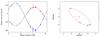 |
Fig. 1 Best-fit orbit compared to the historical RV observations (left) and the new astrometric observations from PIONIER (right). |
The specificity of the present data set is that we have RV data for the two components of the binary and astrometric data of the relative orbital motion. A combined fit of these data allows one to determine unambiguously all masses and orbital parameters of the system. In a standard Keplerian model, the radial velocities vrad,a and vrad,b of the two stellar components and the (x,y) relative astrometric position (projected onto the sky) of component b relative to component a read  Here, Ka and Kb are the individual amplitudes of the RV wobbles of both stars, v0 is the systemic heliocentric offset velocity, e is the orbital eccentricity, and i, Ω and ω stand for the inclination, longitude of ascending node, and argument of periastron of the orbit with respect to a fixed referential frame. The OXYZ referential frame is chosen in such a way that the XOY plane corresponds to the plane of the sky, that the OZ axis points toward the Earth, and that Ω is measured counterclockwise from north (the OX axis is Δδ and points toward north; the OY axis is Δα and points toward east). aapp is the apparent semi-major axis of the astrometric orbit in milli-arcsec, and ν is the current true anomaly along the orbit. ν is related to the time by standard Kepler formalism, via the introduction of the orbital period P (or the orbital angular velocity n) and the time of periastron passage tp.
There are therefore ten independent parameters to fit, namely v0, Ka, Kb, tP, n, e, i, Ω, ω, and aapp. Additional physical quantities can then be derived from the knowledge of these parameters. The RV amplitudes are for instance related to the individual masses Ma and Mb by  (6)where aphy is the physical semi-major axis of the orbit (in AU). Thanks to our astrometric data, the inclination i can be fitted as an independent parameter, so that aphy can be simply deduced from Ka + Kb. Then, with the knowledge of n, the total mass Ma + Mb is derived from Kepler’s third law, and the values of Ka and Kb yield the individual masses Ma and Mb. Finally, the comparison between the physical (aphy) and apparent (aapp) semi-major axes gives access to the distance d of the system.
We performed a combined Levenberg-Marquardt least-square fit of the data. The convergence toward a single and deep χ2 minimum is rapid and robust for a wide range of initial guesses, so that we are confident in our orbital determination. The error bars on the parameters were deduced from their covariance matrix, which is relevant in the present case of a deep minimum where the errors are probably Gaussian. The result of this fit is summarized in Fig. 1 and Table 3.
The very large time separation between the first RV observations (1911) and the last astrometric measurements (2012) allows the orbital period to be determined with a very high accuracy (≈6 s, i.e., ≈5 × 10⁻⁶ relative accuracy). The physical separation corresponds to about 15 stellar radii of the primary. The orbit is compatible with a null eccentricity, because the error bar on the eccentricity is comparable to the fitted value. Consequently, the ω parameter is meaningless and unconstrained. The estimated distance to the system is compatible with the Hipparcos parallax for this star 16.71 ± 0.27 mas = 59.8 ± 1 pc (van Leeuwen 2007). The mass of the primary is slightly larger than the photometric estimate Ma = 2.72 M⊙ from Guthrie (1986).
Best-fit orbital elements and related physical parameters.
 |
Fig. 2 Observed SED of the integrated flux of the binary (gray points), modeled by a sum of two Kurucz models with the stellar parameters described in Sect. 3 (solid black line). The red and blue circles are the flux of the primary and the secondary obtained by combining the observed flux ratio with the total flux at nearby wavelengths. These points are lowered by half a decade for clarity purpose. The dashed lines represent the flux of the corresponding Kurucz models. |
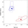 |
Fig. 3 Solid lines are the 3σ confidence regions (blue for the primary and red for the secondary) when adjusting the photometry and the flux ratio with Kurucz models. The dot, dashed and dash-dot lines are the confidence region derived from the studies of Smith & Dworetsky (1993), Wahlgren et al. (1994), and Hubrig et al. (1999) respectively. The filled stars are the adopted stellar parameters. |
3. Temperatures, sizes, and age
We retrieved the observed spectral energy distribution (SED) of the sum of the two components using the tool VOSpec3 provided by the ESA Virtual Observatory (data coming from the following catalogs: IUE for the UV, Johnson and SDSS for the optical, 2MASS for the near-infrared, and IRAS for the infrared). In addition, the interferometric observations presented in the previous section constrain the flux ratio to be 2.9 ± 0.1 in the H band (1.63 μm). From spectroscopic analysis in the optical, Wahlgren et al. (1994) determined a slightly higher flux ratio of 3.92 at 0.44 μm and 3.62 at 0.6 μm. All these measurements are reported in Fig. 2.
We built synthetic SEDs for each component using the DFSYNTHE, KAPPA9, ATLAS9, and SYNTHE codes and tables (Kurucz 1991; Sbordone et al. 2004; Castelli 2005). We used the GNU/LINUX port from Sbordone4 and Castelli5. For the primary, we furthermore computed a custom opacity density function (ODF) table using the abundances published by Wahlgren et al. (1994) before running the ATLAS9 code. The surface gravity of the models were adjusted to correspond to the masses estimated in Sect. 2 although the impact on the result is very small. We used the distance estimated in the previous section to compute the apparent fluxes. Typical values for the interstellar extinction in the solar neighborhood give an extinction of A(V) = 0.05, which has negligible impact on the results.
The diameters and effective temperatures of both components were adjusted so that the predictions from the models match the integrated photometric measurement and the available flux ratio. We explored a grid of diameters from one to four solar radii and temperatures from 6000 K to 15 000 K. The result in shown in Fig. 3. The confidence regions of our adjustment are represented by the solid lines. The results for the secondary are partially degenerated because the measurements of the flux ratio lie in the Rayleigh-Jeans domain.
Several estimates of the effective temperatures and the surface gravities for this system exist in the literature, generally using Strömgren and Geneva photometry. Smith & Dworetsky (1993) measured the stellar parameters of the primary component and found Ta = 10 750 K and log (ga) = 4.0. Wahlgren et al. (1994) iteratively determined the parameters of the two components by a detailed spectroscopic modeling and obtained Ta = 10 650 K, Tb = 9200 K, log (ga) = 3.89 and log (gb) = 4.2. Hubrig et al. (1999) found Ta = 10 664 ± 400 K and log (ga) = 4.22 ± 0.05, when fixing the parameters of the secondary to Tb = 9200 K and log (gb) = 4.2 (taken from Wahlgren et al. (1994)). Our independent determination of the masses of each component allows us to convert the surface gravity g and the mass M into the physical radius R of the photosphere: 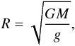 (7)where G is the gravitational constant. The resulting confidence region in effective temperature and radii are represented by the dot, dashed, and dashed-dot lines in Fig. 3. When no other information is given in the literature, we assumed an uncertainty of ± 250 K on the temperature and ± 0.1dex on the log (g). The error boxes overlay adequately with our confidence regions.
To better constrain the stellar radii we decided to adopt the effective temperature of the primary determined from spectroscopy by Wahlgren et al. (1994), i.e. Ta = 10 650 K. Doing so, we obtained a best fit with Tb = 9100 K, Ra = 2.85 ± 0.15 R⊙ and Rb = 1.75 ± 0.18 R⊙. Assuming an uncertainty of ± 250 K on the effective temperature of the primary does not significantly modify the stellar radii. The resulting modeled SED is displayed in Fig. 2, together with the available measurements. Our revision of the stellar radii lead to a ratio Ra / Rb = 1.63 ± 0.08. This is in reasonable agreement with the value Ra / Rb = 1.67 derived by Wahlgren et al. (1994) from the spectroscopic flux ratio. The flux ratio in the B, R, and H bands are all correctly reproduced. Since the latter is a direct and fully independent measurement, it validates a posteriori the flux ratio used in the abundance studies from Leckrone et al. (1999), Brandt et al. (1999), and Nielsen et al. (2005).
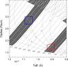 |
Fig. 4 Evolutionary tracks from Mowlavi et al. (2012) for slightly sub-solar initial metallicity (Z = 0.012). Dashed lines are isochrones for ages from 1 to 5 × 10⁸ years. The gray regions correspond to tracks compatible with the dynamical masses estimated in Sect. 2. The colored boxes are the effective temperatures and stellar radii discussed in Sect. 3. |
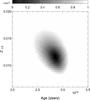 |
Fig. 5 Map of Log(χ2) versus initial metalicity (vertical axis) and age of the system (horizontal axis) when comparing the effective temperatures and radii to the prediction of the evolutionary tracks from Mowlavi et al. (2012). We used the dynamical masses estimated in Sect. 2 and assumed coevality and identical initial metallicity for the two components. |
We then compared our estimates of the effective temperatures and stellar radii with predictions from evolutionary tracks computed for the masses determined in Sect. 2. This is shown in Fig. 4. The confidence boxes represent the intersection of the different constraints from Fig. 3. We used the tracks from Mowlavi et al. (2012) and a slightly sub-solar initial metallicity Z = 0.012. For both components, the confidence boxes overlap correctly with the evolutionary tracks. We explored how sensitive the agreement is to the chosen initial metallicity. We performed a grid of {Age, Z}, and compared the predicted radii and effective temperature to the observations. Doing so, we assumed that the two components are coeval and have the same initial metallicity. These are realistic assumptions for such a tight binary of massive stars, whose probability to result from a capture is extremely low. The resulting χ2 map is shown in Fig. 5. Every initial metallicity in the range Z = 0.009 to 0.014 provides a correct agreement between the tracks and the boxes, and respects coevality. The best agreement is formally found for an initial metallicity Z = 0.0115 and an age of 2.85 × 10⁸ years.
Angular rotation velocities, assuming the radii determined in the present work and vsinir values from the literature.
4. Circularization and synchronization
The mechanisms responsible for the development of the chemical anomalies in the stellar atmosphere of HgMn stars are not yet fully understood. Slow rotational velocities are definitely the most important ingredients. For HD 141556, the existing studies all found low small rotational velocities but disagree on the exact values (see Table 4). Measuring such a small broadening is indeed challenging. However, we note that the vsinir are still higher than the microturbulent velocities (ξa = 0 km s-1 and ξb = 2 km s-1, Wahlgren et al. (1994)). This makes us confident that the measured rotational velocities are, at least, reliable upper limits. The literature provides no uncertainties for these quantities and we used instead the dispersion of the existing measurements.
It is worth questioning, then, whether the system has reached such low rotational velocities by means of synchronisation between rotation and orbital motion, thanks to past or still present tidal interaction. To do this, we need to compare the true angular rotation velocities of the stars with the orbital angular velocity n = 4.7 μrad s-1.
Tides in a binary system usually act to align and synchronize spins with orbital motion and at circularizing the orbit. It is well known that spin alignement and synchronization are usually achieved before circularization. The virtually zero eccentricity of the pair is an indication for an already achieved tidal circularization, and thus spin alignement and synchronization. Consequently, we may reasonably assume that the stars have rotation axes perpendicular to their orbital plane (zero obliquities, ir = i). With this assumption and our knowledge of the stellar radii, it is then possible to derive the angular rotation velocities Na and Nb of the stars: 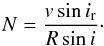 (8)The results are displayed in Table 4. An exact synchronism would imply Na = Nb = n. While the secondary could appear to be synchronized within the error bars, obviously the primary rotates sub-synchronously with respect to the orbital motion. Sub-synchronism is rare among short-period binaries, but some cases have already been reported (Casey et al. 1995; Fekel et al. 2011). Strikingly, the occurence of sub-synchronism seems to be higher in binaries with an HgMn component (Guthrie 1986; Hubrig & Mathys 1995). Hence it is interesting to study the history of synchronization in the HD 141556 system.
There are different theories for tides in close binary stars that provide predictions for synchronization and circularization times. The first one is the equilibrium tide, where each component, distorted by the other, reaches an equilibrium figure. Then the viscosity prevents the equilibrium bulges from permanently pointing toward each other. The result is a coupling between rotation and orbital motion. This theory was first described in detail by Alexander (1973). The synchronization and circularization times depend on the mean viscosity of the stars, which are poorly constrained parameters. But Press et al. (1975) showed that in radiative envelopes, turbulent viscosity dominates, and the authors deduced explicit formulas.
Zahn (1975) introduced another mechanism called dynamical tides that mainly applies to stars with radiative envelopes. In these stars, non-adiabatic oscillations driven by one component onto the other are damped by radiative dissipation, which causes a torque that is responsible for coupling between rotation and orbital motion. Zahn (1977) gives characteristic times.
A third mechanism was introduced by Tassoul & Tassoul (1992) and is based on tidally driven meridional currents within the stars. According to these authors, this purely hydrodynamical mechanism can naturally explain the high degree of synchronism and circularization observed among close early-type and late-type binaries. They provide characteristic times for synchronization and circularization that mainly depend on the masses, sizes, luminosity, and separation of the components.
Characteristic times for the different tidal mechanisms, computed at ZAMS.
The characteristic times are summarized in Table 5, while the details of the computation can be found in the appendix. The difficulty is always to estimate the various characteristic constants that appear in these formulas. Note that the actual circularization time is computed from the two separate circularization times 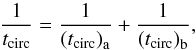 (9)because the contributions of both stars to the circularization process are added.
The mechanism proposed by Tassoul & Tassoul (1992) is by far the fastest, as already noted by Beust et al. (1997). However, the reality of this mechanism is questioned (Rieutord & Zahn 1997). We also note that dynamical tides are more efficient than equilibrium tides. This agrees with Zahn (2008), who stressed that dynamical tides are the dominant mechanism in stars with an outer radiative envelope (which is the case here), and that equilibrium tides are stronger for stars with a convective envelope and for planets.
What conclusion can we derive for the HD 141556 system? First, we note that irrespective of the mechanism, circularization is not expected to be achieved at the age of the system. This could appear to be surprising given the eccentricity we measure, but it is worth recalling that the strength of the tides is highly time-variable. Basically, for such stars, tides are expected to be much stronger in the pre-main sequence (PMS) phase, thanks to the presence of convective envelopes. Circularization is therefore very likely to have enough time to be reached during the PMS phase. But in that case, the stars should also meanwhile have synchronized their rotations. Second, we stress that if the Tassoul & Tassoul (1992) mechanism were active today, both stars would still be perfectly synchronized. The synchronization times associated to this mechanism are indeed very short. Hence any departure from synchronism should be quickly damped by meridional circulation. Thus the observed sub-synchronism of the primary (whatever its origin) indicates that meridional circulation is very likely inactive in this pair.
Our proposed scenario is then the following: in the PMS phase, the tidal coupling of these stars was strong. It could be due to both dynamical and equilibrium tides. This strong coupling resulted in a rapid synchronization and circularization of the pair. Then, after the zero-age main-sequence (ZAMS) and the settling of a radiative envelope, the tidal coupling dropped drastically. In the absence of any external perturbation to the orbit, the eccentricity remained low. But between ZAMS and today, both stars underwent a significant radius increase. With our knowledge of the current radii and of the radii at ZAMS (Fig. 4), we can compute the expected angular velocities for the present day Nnow = n (Rzams / Rnow)2. This formula assumes perfect synchronism at the ZAMS, conservation of the rotational angular momenta between ZAMS and now, and no change in the internal structures of the stars. We found Na = 1.9 μrad s-1 and Nb = 3.5 μrad s-1. These values are still slightly higher than that of Table 4, but, at first order, this simplistic scenario provides a plausible explanation for the sub-synchronism of the two components.
We stress that there is no definite theory for the explanation of sub-synchronous rotation. A classical scenario for slowing down stars is of course a magnetic field. The existence of an efficient magnetic braking has been proposed to explain why all the magnetic A stars (Ap) have very slow rotational velocities. In binary system, such a magnetic braking could overcome the tidal synchronisation and naturally lead to sub-synchronous rotation (Hubrig & Mathys 1995). This is especially true for HD 141556 because the tidal coupling seems weak according to the calculation presented above. However, this scenario requires that the two components are, or were at some point, strongly magnetized. Moreover, it does not explain the almost perfect circularization of the orbit.
5. Concluding remarks
HD 141556 is a promising target for a precision test of evolutionary models with chemically peculiar stars. Accurate radial velocity measurements (according to modern standards) and a few additional interferometric observations spread over the orbital cycle should considerably reduce the mass uncertainties, which are currently at the ≈5% level. A single interferometric observation in the visible could provide a direct estimate of the flux ratio in this band (existing estimates rely on spectroscopic analysis), which should help in constraining the temperatures and the ratio of radii. A direct measurement of the stellar diameters (0.43 mas) is within reach with the SUSI interferometer or a next-generation optical instrument at VLTI.
Our proposed scenario to explain the current rotation velocities implies that the stars have been synchronized by tidal coupling in the final stage of contracting toward the zero-age main sequence, and then fully decoupled during their evolution on the main sequence. Adding generality to this result, it supports the fact that many HgMn stars are found in young multiple systems and in young associations. It is conceivable that these stars have been synchronized and that their peculiarities were established as early as the pre-main sequence phase. A quantitative test of this scenario requires modeling the internal structure of the two stars at all times, including the pre-main sequence.
Online material
Appendix A: Interferometric observations
 |
Fig. A.1 Square visibilities (left), closure phases (middle) and corresponding reduced χ2 map (right) for the PIONIER observation of 2012-02-24. The corresponding best-fit binary model is shown in red. |
Appendix B: Computation of characteristic times for circularization and synchronization
Appendix B.1: Equilibrium tide
Press et al. (1975) provide explicit formulas. For each component of the binary, we have 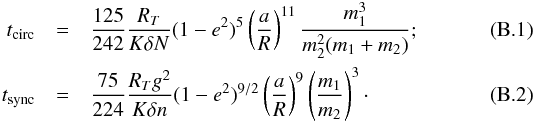 Here N is the angular rotation velocity of the star, g is its gyration radius (the moment of inertia is defined as g2mR2), RT is an effective Reynolds number that can be taken ~20, and K and δ are numerical parameters. According to Press et al. (1975), we can typically assume K = 0.025 and δ = 0.1. The other symbols have their meaning introduced above. These formulas are valid for either component of the binary. In each case, m1 stands for the mass of the star we are considering, and m2 for the mass of the other star.
Appendix B.2: Dynamical tides
Zahn (1977) gave characteristic times. 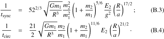
The conventions are the same as above. E2 is a dimensionless constant characteristizing the strength of the dynamical tide. Zahn (1975) provided a table of E2 and gyration radius at ZAMS for various masses. We interpolated these values for the actual masses and computed the characteristic times, assuming n = N and e = 0.
Appendix B.3: Tidally driven meridional currents
According to Tassoul & Tassoul (1992), the characteristic times in years are 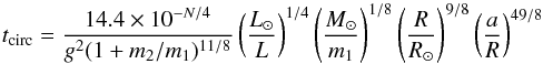 (B.5)and
 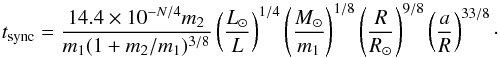 (B.6)L is the stellar luminosity and N is a charateristic exponent that can be taken as 10 for stars with a convective envelope, and 0 for stars with a radiative envelope, which is the case here.
Acknowledgments
PIONIER is funded by the Université Joseph Fourier (UJF, Grenoble) through its Poles TUNES and SMING and the vice-president of research, the Institut de Planétologie et d’Astrophysique de Grenoble, the “Agence Nationale pour la Recherche” with the program ANR EXOZODI, and the Institut National des Sciences de l’Univers (INSU) with the programs “Programme National de Physique Stellaire” and “Programme National de Planétologie”. The integrated optics beam combiner is the result of a collaboration between IPAG and CEA-LETI based on CNES R&T funding. FMe acknowledges support from EU FP7-2011 under grant agreement No. 284405 (DIANA) and from the Milenium Nucleus P10-022-F, funded by the Chilean Government. The authors want to warmly thank all the people involved in the VLTI project. It made use of the Smithsonian/NASA Astrophysics Data System (ADS), of the Centre de Données astronomiques de Strasbourg (CDS) and of the Jean-Marie Mariotti Center (JMMC). Some calculations and graphics were performed with the freeware Yorick.
References
- Abt, H. A., Chaffee, F. H., & Suffolk, G. 1972, ApJ, 175, 779 [Google Scholar]
- Alexander, M. E. 1973, Ap&SS, 23, 459 [NASA ADS] [CrossRef] [Google Scholar]
- Beust, H., Corporon, P., Siess, L., Forestini, M., & Lagrange, A.-M. 1997, A&A, 320, 478 [Google Scholar]
- Brandt, J. C., Heap, S. R., Beaver, E. A., et al. 1999, AJ, 117, 1505 [NASA ADS] [CrossRef] [Google Scholar]
- Casey, B. W., Mathieu, R. D., Suntzeff, N. B., & Walter, F. M. 1995, AJ, 109, 2156 [NASA ADS] [CrossRef] [Google Scholar]
- Castelli, F. 2005, Mem. Soc. Astron. It. Suppl., 8, 34 [Google Scholar]
- Dworetsky, M. M. 1972, PASP, 84, 254 [NASA ADS] [CrossRef] [Google Scholar]
- Fekel, F. C., Williamson, M. H., & Henry, G. W. 2011, AJ, 141, 145 [NASA ADS] [CrossRef] [Google Scholar]
- Guthrie, B. N. G. 1986, MNRAS, 220, 559 [NASA ADS] [Google Scholar]
- Haguenauer, P., Alonso, J., Bourget, P., et al. 2010, in SPIE Conf. Ser. 7734 [Google Scholar]
- Hubrig, S., & Mathys, G. 1995, in Laboratory and Astronomical High Resolution Spectra, eds. A. J. Sauval, R. Blomme, & N. Grevesse, ASP Conf. Ser., 81, 555 [Google Scholar]
- Hubrig, S., Castelli, F., & Mathys, G. 1999, A&A, 341, 190 [NASA ADS] [Google Scholar]
- Hubrig, S., González, J. F., Ilyin, I., et al. 2012, A&A, 547, A90 [NASA ADS] [CrossRef] [EDP Sciences] [Google Scholar]
- Kurucz, R. L. 1991, in Stellar Atmospheres − Beyond Classical Models, eds. L. Crivellari, I. Hubeny, & D. G. Hummer, NATO ASIC Proc., 341, 441 [Google Scholar]
- Lafrasse, S., Mella, G., Bonneau, D., et al. 2010, in SPIE Conf. Ser., 7734 [Google Scholar]
- Le Bouquin, J.-B., Berger, J.-P., Lazareff, B., et al. 2011, A&A, 535, A67 [NASA ADS] [CrossRef] [EDP Sciences] [Google Scholar]
- Leckrone, D. S., Proffitt, C. R., Wahlgren, G. M., Johansson, S. G., & Brage, T. 1999, AJ, 117, 1454 [NASA ADS] [CrossRef] [Google Scholar]
- Mathys, G., & Hubrig, S. 1995, A&A, 293, 810 [NASA ADS] [Google Scholar]
- Michaud, G. 1970, ApJ, 160, 641 [NASA ADS] [CrossRef] [Google Scholar]
- Michaud, G., Reeves, H., & Charland, Y. 1974, A&A, 37, 313 [NASA ADS] [Google Scholar]
- Mowlavi, N., Eggenberger, P., Meynet, G., et al. 2012, A&A, 541, A41 [NASA ADS] [CrossRef] [EDP Sciences] [Google Scholar]
- Nielsen, K. E., Wahlgren, G. M., Proffitt, C. R., Leckrone, D. S., & Adelman, S. J. 2005, AJ, 130, 2312 [NASA ADS] [CrossRef] [Google Scholar]
- Press, W. H., Smarr, L. L., & Wiita, P. J. 1975, ApJ, 202, L135 [NASA ADS] [CrossRef] [Google Scholar]
- Preston, G. W. 1974, ARA&A, 12, 257 [NASA ADS] [CrossRef] [MathSciNet] [Google Scholar]
- Proffitt, C. R. 2002, ApJ, 571, 955 [NASA ADS] [CrossRef] [Google Scholar]
- Rieutord, M., & Zahn, J.-P. 1997, ApJ, 474, 760 [NASA ADS] [CrossRef] [Google Scholar]
- Sbordone, L., Bonifacio, P., Castelli, F., & Kurucz, R. L. 2004, Mem. Soc. Astron. It. Suppl., 5, 93 [Google Scholar]
- Schöller, M., Correia, S., Hubrig, S., & Ageorges, N. 2010, A&A, 522, A85 [NASA ADS] [CrossRef] [EDP Sciences] [Google Scholar]
- Smith, K. C., & Dworetsky, M. M. 1993, A&A, 274, 335 [NASA ADS] [Google Scholar]
- Tallon-Bosc, I., Tallon, M., Thiébaut, E., et al. 2008, in SPIE Conf. Ser., 7013 [Google Scholar]
- Tassoul, J.-L., & Tassoul, M. 1992, ApJ, 395, 259 [NASA ADS] [CrossRef] [Google Scholar]
- van Leeuwen, F. 2007, A&A, 474, 653 [NASA ADS] [CrossRef] [EDP Sciences] [Google Scholar]
- Wahlgren, G. M., Adelman, S. J., & Robinson, R. D. 1994, ApJ, 434, 349 [NASA ADS] [CrossRef] [Google Scholar]
- Zahn, J.-P. 1975, A&A, 41, 329 [NASA ADS] [Google Scholar]
- Zahn, J.-P. 1977, A&A, 57, 383 [NASA ADS] [Google Scholar]
- Zahn, J.-P. 2008, in EAS Publ. Ser. 29, eds. M.-J. Goupil, & J.-P. Zahn, 67 [Google Scholar]
All Tables
Log of interferometric observations with PIONIER at the VLTI together with the measured astrometric positions of b (faintest) with respect to a (brightest) and flux ratio in the H band.
Angular rotation velocities, assuming the radii determined in the present work and vsinir values from the literature.
All Figures
|
Fig. 1 Best-fit orbit compared to the historical RV observations (left) and the new astrometric observations from PIONIER (right). |
| In the text | |
|
Fig. 2 Observed SED of the integrated flux of the binary (gray points), modeled by a sum of two Kurucz models with the stellar parameters described in Sect. 3 (solid black line). The red and blue circles are the flux of the primary and the secondary obtained by combining the observed flux ratio with the total flux at nearby wavelengths. These points are lowered by half a decade for clarity purpose. The dashed lines represent the flux of the corresponding Kurucz models. |
| In the text | |
|
Fig. 3 Solid lines are the 3σ confidence regions (blue for the primary and red for the secondary) when adjusting the photometry and the flux ratio with Kurucz models. The dot, dashed and dash-dot lines are the confidence region derived from the studies of Smith & Dworetsky (1993), Wahlgren et al. (1994), and Hubrig et al. (1999) respectively. The filled stars are the adopted stellar parameters. |
| In the text | |
|
Fig. 4 Evolutionary tracks from Mowlavi et al. (2012) for slightly sub-solar initial metallicity (Z = 0.012). Dashed lines are isochrones for ages from 1 to 5 × 10⁸ years. The gray regions correspond to tracks compatible with the dynamical masses estimated in Sect. 2. The colored boxes are the effective temperatures and stellar radii discussed in Sect. 3. |
| In the text | |
|
Fig. 5 Map of Log(χ2) versus initial metalicity (vertical axis) and age of the system (horizontal axis) when comparing the effective temperatures and radii to the prediction of the evolutionary tracks from Mowlavi et al. (2012). We used the dynamical masses estimated in Sect. 2 and assumed coevality and identical initial metallicity for the two components. |
| In the text | |
|
Fig. A.1 Square visibilities (left), closure phases (middle) and corresponding reduced χ2 map (right) for the PIONIER observation of 2012-02-24. The corresponding best-fit binary model is shown in red. |
| In the text | |
 |
Fig. A.2 Same as Fig. A.1 for the PIONIER observation of 2012-03-02. |
| In the text | |
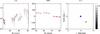 |
Fig. A.3 Same as Fig. A.1 for the PIONIER observation of 2012-03-03. |
| In the text | |
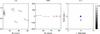 |
Fig. A.4 Same as Fig. A.1 for the PIONIER observation of 2012-03-05. |
| In the text | |
Current usage metrics show cumulative count of Article Views (full-text article views including HTML views, PDF and ePub downloads, according to the available data) and Abstracts Views on Vision4Press platform.
Data correspond to usage on the plateform after 2015. The current usage metrics is available 48-96 hours after online publication and is updated daily on week days.
Initial download of the metrics may take a while.