© ESO, 2013

1. Introduction

Statistical information about the motions of stars relative to the sun may contain important hints concerning the origin and history of the stars themselves (e.g., by identifying kinematic populations and streams) as well as of the physical properties of the Galaxy (through dynamical interpretation of the motions). Ideally this requires that all six components of phase space (positions and velocities) are known for all the stars in the investigated sample. This can in principle be achieved through a combination of astrometric data (providing positions and distances, from the parallaxes, and tangential velocities from the proper motions and parallaxes) and spectroscopic radial velocities. Very often, however, such complete data are not available for all the stars in a sample. For example, the Hipparcos Catalogue (ESA 1997) gives the required astrometric information for large samples of nearby stars, but not all of them have known radial velocities. Restricting the investigation to stars with measured radial velocities could introduce a serious selection bias (Binney et al. 1997). The Gaia mission (de Bruijne 2012) will not only provide vastly improved astrometric data for much larger stellar samples, but also radial-velocity measurements for stars brighter than  ≃ 17 mag; for the fainter stars, however, the phase space data will still be incomplete. On the other hand, on-going spectroscopic surveys such as RAVE (Steinmetz et al. 2006) already provide radial velocities for large samples without the complementary astrometry. Thus we are often faced with the problem to estimate kinematical parameters (such as mean velocities and velocity dispersions) from incomplete phase space data, lacking either the radial or tangential velocity components, or the accurate distances needed to derive the tangential velocities from proper motions.

Dehnen & Binney (1998) derive a simple and elegant method to derive local stellar kinematics (mean velocity and velocity dispersion) for a group of stars, when the tangential velocities are known, but not the radial velocities. This method has become popular and can be considered a standard for this purpose. We will refer to it as the projection method (PM) throughout this paper. In addition to the original work by Dehnen & Binney (1998), the same method (or variants of it) has been used, e.g., by Mignard (2000), Brosche et al. (2001), van Leeuwen (2007), and Aumer & Binney (2009).

Despite its wide usage in the literature, the projection method is not founded on any particular estimation principle such as maximum likelihood (ML) or Bayesian estimation, but simply fit the projected first and second moments of the space velocities to the corresponding observed moments of the tangential velocities. This works well for large samples, provided that the observational uncertainties in the data are negligible compared to the uncertainties due to the sampling, but there is no guarantee that it is unbiased, or asymptotically efficient as expected for an ML estimate. On the contrary, by neglecting the observational errors the resulting velocity dispersions are probably overestimated. Moreover, for small samples the projection method may sometimes give unphysical results, in that the estimated dispersion tensor is not positive-definite – implying that the mean square velocity is negative in some directions. Since it is desirable that the kinematic parameters can be consistently and efficiently estimated also for small samples and in the presence of non-negligible observational uncertainties, we introduce here a new and more rigorous approach, based on the maximum likelihood method.

2. Kinematic parameters and the projection method

For a homogeneous population of stars the phase space density f(r,v,t) describes the density of stars as a function of position (r), velocity (v) and time t. By the local kinematics we mean the distribution function here (r = 0) and now (t = 0), that is f(v) ≡ f(0,v,0). It is usually assumed that f(v) is a smooth function, and the most common assumption is the Schwarzschild approximation, that f(v) is a three-dimensional Gaussian distribution (velocity ellipsoid), or a combination of a few Gaussian distributions. The velocity ellipsoid is completely described by the mean velocity v and the dispersion tensor D.

Throughout this paper we use heliocentric galactic coordinates (x,y,z) with  + x pointing towards the Galactic Centre,  + y in the direction of rotation at the Sun, and  + z towards the north Galactic pole. The corresponding heliocentric velocity components are denoted (v_x,v_y,v_z) or (u,v,w).

For a stellar population, the mean velocity and dispersion tensor are defined as $\begin{array}{ccc}{v̅}& \mathrm{=}& \\ \mathbf{D}& \mathrm{=}& \end{array}$where E is the expectation operator (population mean). Given the 3-dimensional velocities v_i, i = 1,   2,   ...,   n for a sample of stars it is possible to estimate the population mean values by the sample mean values, $\overline{{v}}\mathrm{\simeq }\frac{\mathrm{1}}{\mathit{n}}\sum _{\mathit{i}}{v}\mathit{i}\hspace{0.17em}\mathit{,} \mathbf{D}\mathrm{\simeq }\frac{\mathrm{1}}{\mathit{n}}\sum _{\mathit{i}}\mathrm{(}{v}\mathit{i}\mathrm{-}\overline{{v}}\mathrm{)}\mathrm{(}{v}\mathit{i}\mathrm{-}\overline{{v}}{\mathrm{)}}^{\mathrm{T}}\mathit{.}$(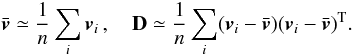3)Note that this estimate of D is always positive definite (except in trivial degenerate cases), but it requires 3-dimensional velocities and the dispersions are likely to be overestimated when the velocity components have significant observational errors.

The tangential velocity of a star can be written ${\tau }\mathrm{=}\mathbf{A}{v}\mathit{,}$(4)where A is a projection matrix depending only on the position of the star. In the projection method the assumption that the positions (and hence the matrices A) are uncorrelated with the velocities is invoked to derive a relation between the mean of τ and the mean of A, allowing the latter to be solved. In a similar way, the elements of D are derived from the relation between the second moments of τ and v. For further details we refer to the paper by Dehnen & Binney (1998).

3. Maximum likelihood estimation of the kinematic parameters

3.1. Overview of the model

We assume a Gaussian distribution of the velocities in all directions. That is, the velocity of a star follows a 3-dimensional normal distribution, ${v}\mathrm{~}{N}\mathrm{\left(}\overline{{v}}\mathit{,}\mathbf{D}\mathrm{\right)}$¹. Given the position and true parallax p of the star we can calculate its true proper motion in longitude and latitude (μ_l,μ_b). Adding Gaussian observational errors to these we get the observed proper motions $\begin{array}{}{}_{\mathrm{˜}}\\ {\mathit{\mu }}_{\mathit{l}}\end{array}\mathrm{~}\mathit{N}\mathrm{\left(}{\mathit{\mu }}_{\mathit{l}}\mathit{,}{\mathit{\sigma }}_{\mathit{\mu }}^{\mathrm{2}}\mathrm{\right)}$, $\begin{array}{}{}_{\mathrm{˜}}\\ {\mathit{\mu }}_{\mathit{b}}\end{array}\mathrm{~}\mathit{N}\mathrm{\left(}{\mathit{\mu }}_{\mathit{b}}\mathit{,}{\mathit{\sigma }}_{\mathit{\mu }}^{\mathrm{2}}\mathrm{\right)}$ and the observed parallax $\begin{array}{}{}_{\mathrm{˜}}\\ \mathit{p}\end{array}\mathrm{~}\mathit{N}\mathrm{\left(}\mathit{p,}{\mathit{\sigma }}_{\mathit{p}}^{\mathrm{2}}\mathrm{\right)}$. The observational uncertainties σ_μ and σ_p are assumed to be known. The ML formulation requires that the probability density function of the observed data $\mathrm{\left(}\begin{array}{}{}_{\mathrm{˜}}\\ {\mathit{\mu }}_{\mathit{l}}\end{array}\mathit{,}\begin{array}{}{}_{\mathrm{˜}}\\ {\mathit{\mu }}_{\mathit{b}}\end{array}\mathit{,}\begin{array}{}{}_{\mathrm{˜}}\\ \mathit{p}\end{array}\mathrm{\right)}$ is written as a function of the model parameters.

3.2. Exact expression for the likelihood

For a problem involving n stars, the parameters of the model are:

• $\overline{{v}}\mathrm{=}$ the mean velocity of the stellar population (a 3-vector, or 3 × 1 matrix);

• D =  the dispersion tensor of the stellar population (a symmetric 3 × 3 matrix; contains 6 non-redundant elements);

• p =  the true parallaxes of the stars (an n-vector, or n × 1 matrix).

It is necessary to introduce the true parallaxes p_i as formal model parameters, although the strategy is that they will be eliminated on a star-by-star basis leaving us with a problem with only nine model parameters, namely the (non-redundant) components of $\overline{{v}}$ and D. We denote by the vector θ the complete set of model parameters (i.e., the unknowns to be estimated). For n stars the total number of model parameters is n + 9.

The observables are, for each star i = 1...n, the observed components of proper motion, $\begin{array}{}{\mathrm{˜}}_{}\\ {\mathit{\mu }}_{\mathit{l,i}}\end{array}$ and $\begin{array}{}{\mathrm{˜}}_{}\\ {\mathit{\mu }}_{\mathit{b,i}}\end{array}$, and the observed parallax $\begin{array}{}{\mathrm{˜}}_{}\\ {\mathit{p}}_{\mathit{i}}\end{array}$. The total number of observables is 3n. These have observational uncertainties that are given by the 3 × 3 covariance matrix C_i. Sometimes it is useful to denote by the vector x the complete set of observables (or data).

Given the observations, the likelihood function $\mathit{L}\mathrm{\left(}{\theta }\mathrm{\right)}\mathrm{\equiv }\mathit{L}\mathrm{\left(}\overline{{v}}\mathit{,}\mathbf{D}\mathit{,}{p}\mathrm{\right)}$ numerically equals the probability density function (pdf) f_x(x | θ) of the observables x, given the model parameters θ. The objective is to find the ML estimate of θ, denoted $\hat{{\theta }}$, i.e., the (hopefully unique) set of parameter values that maximizes L(θ) or, equivalently, the log-likelihood ℓ(θ) = lnL(θ). The total log-likelihood function is given by $\mathit{\ell }\mathrm{\left(}\overline{{v}}\mathit{,}\mathbf{D}\mathit{,}{p}\mathrm{\right)}\mathrm{=}\sum _{\mathit{i}}\mathrm{\left[}\ln {\mathit{f}}_{\begin{array}{}\mathrm{˜}\\ {\mu }\end{array}\mathit{,i}}\mathrm{\right(}{\begin{array}{}\mathrm{˜}\\ {\mu }\end{array}}_{\mathit{i}}\mathrm{\left|}{\mathit{p}}_{\mathit{i}}\mathrm{\right)}\mathrm{+}\ln {\mathit{g}}_{\mathit{i}}\mathrm{(}\begin{array}{}\mathrm{˜}\\ {\mathit{p}}_{\mathit{i}}\end{array}\mathrm{-}{\mathit{p}}_{\mathit{i}}{\mathrm{\left)}}^{\mathrm{\right]}}\hspace{0.17em}\mathit{,}$(5)where g_i is the centered normal pdf with standard deviation ${\mathit{\sigma }}_{\mathit{p,i}}\mathrm{=}\mathrm{[}{\mathbf{C}}_{\mathit{i}}{\mathrm{]}}_{\mathrm{33}}^{\mathrm{1}\mathit{/}\mathrm{2}}$, i.e., the uncertainty of the parallax p_i. It is clear that the parameter p_i only affects the ith term in the sum above. Therefore, when maximizing with respect to p_i we only need to consider that one term. For simplicity we drop, for the moment, the subscript i so that the term to consider (for one star) can be written: $\begin{array}{ccc}\mathit{\ell }\mathrm{\left(}\overline{{v}}\mathit{,}\mathbf{D}\mathit{,p}\mathrm{\right)}& \mathrm{=}& \ln {\mathit{f}}_{\begin{array}{}\mathrm{˜}\\ {\mu }\end{array}}\mathrm{\left(}\begin{array}{}\mathrm{˜}\\ {\mu }\end{array}\mathrm{\right|}\mathit{p}\mathrm{)}\mathrm{+}\ln \mathit{g}\mathrm{(}\begin{array}{}\mathrm{˜}\\ \mathit{p}\end{array}\mathrm{-}\mathit{p}\mathrm{)}\\ & \mathrm{=}& \ln {\mathit{f}}_{\begin{array}{}\mathrm{˜}\\ {\mu }\end{array}}\mathrm{\left(}\begin{array}{}\mathrm{˜}\\ {\mu }\end{array}\mathrm{\right|}\mathit{p}\mathrm{)}\mathrm{-}\frac{\mathrm{1}}{\mathrm{2}}\ln \mathrm{(}\mathrm{2}\mathit{\pi }{\mathit{\sigma }}_{\mathit{p}}^{\mathrm{2}}\mathrm{)}\mathrm{-}\frac{\mathrm{(}\mathit{p}\mathrm{-}\begin{array}{}\mathrm{˜}\\ \mathit{p}\end{array}{\mathrm{)}}^{\mathrm{2}}}{\mathrm{2}{\mathit{\sigma }}_{\mathit{p}}^{\mathrm{2}}}\mathit{,}\end{array}$(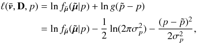6)where we have used 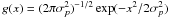$\mathit{g}\mathrm{\left(}\mathit{x}\mathrm{\right)}\mathrm{=}\mathrm{\left(}\mathrm{2}\mathit{\pi }{\mathit{\sigma }}_{\mathit{p}}^{\mathrm{2}}{\mathrm{)}}^{\mathrm{-}\mathrm{1}\mathit{/}\mathrm{2}}\exp \mathrm{\right(}\mathrm{-}{\mathit{x}}^{\mathrm{2}}\mathit{/}\mathrm{2}{\mathit{\sigma }}_{\mathit{p}}^{\mathrm{2}}\mathrm{)}$ for the normal pdf with standard deviation σ_p. Note that ${\mathit{f}}_{\begin{array}{}{}_{\mathrm{˜}}\\ {\mu }\end{array}}\mathrm{\left(}\begin{array}{}{}_{\mathrm{˜}}\\ {\mu }\end{array}\mathrm{\right|}\mathit{p}\mathrm{)}$ of course depends on $\overline{{v}}$ and D as well, although we focus on the dependence on p here. We now need an explicit expression for the pdf ${\mathit{f}}_{\begin{array}{}{}_{\mathrm{˜}}\\ {\mu }\end{array}}\mathrm{\left(}\begin{array}{}{}_{\mathrm{˜}}\\ {\mu }\end{array}\mathrm{\right|}\mathit{p}\mathrm{)}$ of the observed proper motion $\begin{array}{}{\mathrm{˜}}_{}\\ {\mu }\end{array}$ when the true parallax p is known. This is clearly a two-dimensional Gaussian (since both the velocities and the observational errors are Gaussian), with expected value $\mathrm{E}\left[\begin{array}{}\mathrm{˜}\\ {\mu }\end{array}\right]\mathrm{=}\mathbf{M}\overline{{v}}\mathit{.}$(7)Here, M is the 2 × 3 matrix $\mathbf{M}\mathrm{=}\frac{\mathit{p}}{\mathit{K}}\left[\begin{array}{c}\\ \mathrm{-}\sin \mathit{l}& \cos \mathit{l}& \mathrm{0}\\ \mathrm{-}\cos \mathit{l}\sin \mathit{b}& \mathrm{-}\sin \mathit{l}\cos \mathit{b}& \cos \mathit{b}\end{array}\right]$(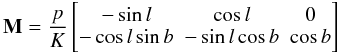8)projecting any vector (in this case $\overline{{v}}$) to its components in the directions of increasing galactic coordinates l and b. The factor p/K converts the velocity to proper motion (numerically, K = 4.7405 if the units used are km s^-1, mas, and mas yr^-1). Assuming that the observational errors are not correlated with the velocities, the covariance of $\begin{array}{}{\mathrm{˜}}_{}\\ {\mu }\end{array}$ is the sum of the covariance due to the velocity dispersion and the covariance due to the observational errors, i.e.: $\mathrm{Cov}\left[\begin{array}{}\mathrm{˜}\\ {\mu }\end{array}\right]\mathrm{\equiv }{\mathbf{C}}_{\begin{array}{}\mathrm{˜}\\ {\mu }\end{array}}\mathrm{=}\mathbf{MD}{\mathbf{M}}^{\mathrm{T}}\mathrm{+}\left[\begin{array}{c}\\ {\mathit{\sigma }}_{\mathit{\mu l}}^{\mathrm{2}}& \mathit{\rho }{\mathit{\sigma }}_{\mathit{\mu l}}{\mathit{\sigma }}_{\mathit{\mu b}}\\ \mathit{\rho }{\mathit{\sigma }}_{\mathit{\mu l}}{\mathit{\sigma }}_{\mathit{\mu b}}& {\mathit{\sigma }}_{\mathit{\mu b}}^{\mathrm{2}}\end{array}\right]\mathit{,}$(9)where σ_μl and σ_μb are the observational uncertainties in μ_l and μ_b, and ρ their correlation coefficient. The pdf is then ${\mathit{f}}_{\begin{array}{}\mathrm{˜}\\ {\mu }\end{array}}\mathrm{\left(}\begin{array}{}\mathrm{˜}\\ {\mu }\end{array}\mathrm{\right|}\mathit{p}\mathrm{)}\mathrm{=}\mathrm{(}\mathrm{2}\mathit{\pi }{\mathrm{)}}^{-1}{\left|{\mathbf{C}}_{\begin{array}{}\mathrm{˜}\\ {\mu }\end{array}}\right|}^{\mathrm{-}\mathrm{1}\mathit{/}\mathrm{2}}\exp \left[\mathrm{-}\frac{\mathrm{1}}{\mathrm{2}}{\left(\begin{array}{}\mathrm{˜}\\ {\mu }\end{array}\mathrm{-}\mathbf{M}\overline{{v}}\right)}^{\mathrm{\prime }}{\mathbf{C}}_{\begin{array}{}\mathrm{˜}\\ {\mu }\end{array}}^{-1}\left(\begin{array}{}\mathrm{˜}\\ {\mu }\end{array}\mathrm{-}\mathbf{M}\overline{{v}}\right)\right]\hspace{0.17em}\mathit{.}$(10)

3.3. Eliminating the parallaxes

The large number of parameters in the likelihood function in Eq. (5) makes it difficult to maximize. We approach this problem by finding the maximum of Eq. (6) with respect to p for each star and thus eliminating p. Since the expression for ${\mathit{f}}_{\begin{array}{}{}_{\mathrm{˜}}\\ {\mu }\end{array}}\mathrm{\left(}\begin{array}{}{}_{\mathrm{˜}}\\ {\mu }\end{array}\mathrm{\right|}\mathit{p}\mathrm{)}$ is quite complicated, it is not likely that this can be done exactly, by analytical means, but we can find an approximate solution valid in the limit of small relative parallax error, σ_p/p ≪ 1.

To eliminate p we take the partial derivative of Eq. (6) with respect to p and set it equal to 0. The result is 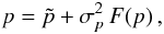$\mathit{p}\mathrm{=}\begin{array}{}\mathrm{˜}\\ \mathit{p}\end{array}\mathrm{+}{\mathit{\sigma }}_{\mathit{p}}^{\mathrm{2}}\hspace{0.17em}\mathit{F}\mathrm{\left(}\mathit{p}\mathrm{\right)}\hspace{0.17em}\mathit{,}$(11)where we introduced for brevity 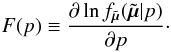$\mathit{F}\mathrm{\left(}\mathit{p}\mathrm{\right)}\mathrm{\equiv }\frac{\mathit{\partial }\ln {\mathit{f}}_{\begin{array}{}\mathrm{˜}\\ {\mu }\end{array}}\mathrm{\left(}\begin{array}{}\mathrm{˜}\\ {\mu }\end{array}\mathrm{\right|}\mathit{p}\mathrm{)}}{\mathit{\partial p}}\mathrm{·}$(12)So far no approximation has been made. However, in Eq. (11) the function F is to be evaluated for the value of p which we are seeking, so we have not really solved the problem. But if σ_p ≪ p we can evaluate F(p) at $\mathit{p}\mathrm{=}\begin{array}{}{}_{\mathrm{˜}}\\ \mathit{p}\end{array}$ to obtain the explicit formula 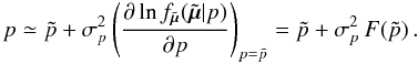$\mathit{p}\mathrm{\simeq }\begin{array}{}\mathrm{˜}\\ \mathit{p}\end{array}\mathrm{+}{\mathit{\sigma }}_{\mathit{p}}^{\mathrm{2}}{\left(\frac{\mathit{\partial }\ln {\mathit{f}}_{\begin{array}{}\mathrm{˜}\\ {\mu }\end{array}}\mathrm{\left(}\begin{array}{}\mathrm{˜}\\ {\mu }\end{array}\mathrm{\right|}\mathit{p}\mathrm{)}}{\mathit{\partial p}}\right)}_{\mathit{p}\mathrm{=}\begin{array}{}\mathrm{˜}\\ \mathit{p}\end{array}}\mathrm{=}\begin{array}{}\mathrm{˜}\\ \mathit{p}\end{array}\mathrm{+}{\mathit{\sigma }}_{\mathit{p}}^{\mathrm{2}}\hspace{0.17em}\mathit{F}\mathrm{\left(}\begin{array}{}\mathrm{˜}\\ \mathit{p}\end{array}\mathrm{\right)}\hspace{0.17em}\mathit{.}$(13)This approximation is safe to do under the assumption of small relative parallax error, since Eq. (13) is obviously correct to first order in ${\mathit{\sigma }}_{\mathit{p}}^{\mathrm{2}}$. Inserting the first-order Taylor expansion $\ln {\mathit{f}}_{\begin{array}{}\mathrm{˜}\\ {\mu }\end{array}}\mathrm{\left(}\begin{array}{}\mathrm{˜}\\ {\mu }\end{array}\mathrm{\right|}\mathit{p}\mathrm{)}\mathrm{\simeq }\ln {\mathit{f}}_{\begin{array}{}\mathrm{˜}\\ {\mu }\end{array}}\mathrm{(}\begin{array}{}\mathrm{˜}\\ {\mu }\end{array}\mathrm{\left|}\begin{array}{}\mathrm{˜}\\ \mathit{p}\end{array}\mathrm{\right)}\mathrm{+}\mathrm{(}\mathit{p}\mathrm{-}\begin{array}{}\mathrm{˜}\\ \mathit{p}\end{array}\mathrm{)}\mathit{F}\mathrm{\left(}\begin{array}{}\mathrm{˜}\\ \mathit{p}\end{array}\mathrm{\right)}$(14)in Eq. (6) and using $\mathit{p}\mathrm{-}\begin{array}{}{}_{\mathrm{˜}}\\ \mathit{p}\end{array}\mathrm{\simeq }{\mathit{\sigma }}_{\mathit{p}}^{\mathrm{2}}\mathit{F}\mathrm{\left(}\begin{array}{}{}_{\mathrm{˜}}\\ \mathit{p}\end{array}\mathrm{\right)}$ from Eq. (13), the log-likelihood maximized with respect to p becomes: $\mathit{\ell }\mathrm{\left(}\overline{{v}}\mathit{,}\mathbf{D}\mathrm{\right)}\mathrm{\simeq }\ln {\mathit{f}}_{\begin{array}{}\mathrm{˜}\\ {\mu }\end{array}}\mathrm{\left(}\begin{array}{}\mathrm{˜}\\ {\mu }\end{array}\mathrm{\right|}\begin{array}{}\mathrm{˜}\\ \mathit{p}\end{array}\mathrm{)}\mathrm{+}\frac{\mathrm{1}}{\mathrm{2}}{\mathit{\sigma }}_{\mathit{p}}^{\mathrm{2}}\hspace{0.17em}\mathit{F}\mathrm{(}\begin{array}{}\mathrm{˜}\\ \mathit{p}\end{array}{\mathrm{)}}^{\mathrm{2}}\hspace{0.17em}\mathit{.}$(15)Here we have neglected the additive constant $\mathrm{-}\frac{\mathrm{1}}{\mathrm{2}}\ln \mathrm{\left(}\mathrm{2}\mathit{\pi }{\mathit{\sigma }}_{\mathit{p}}^{\mathrm{2}}\mathrm{\right)}$, which does not depend on the model parameters and therefore is irrelevant for the ML problem.

Recalling that this is just the log-likelihood term for one star, the total log-likelihood function, after maximization with respect to p, is therefore: $\mathit{\ell }\mathrm{\left(}\overline{{v}}\mathit{,}\mathbf{D}\mathrm{\right)}\mathrm{\simeq }\sum _{\mathit{i}}\left[\ln {\mathit{f}}_{\begin{array}{}\mathrm{˜}\\ {\mu }\end{array}\mathit{,i}}\mathrm{\left(}{\begin{array}{}\mathrm{˜}\\ {\mu }\end{array}}_{\mathit{i}}\mathrm{\right|}{v̅}\mathit{,}\mathbf{D}\mathit{,}\begin{array}{}\mathrm{˜}\\ {\mathit{p}}_{\mathit{i}}\end{array}\mathrm{)}\mathrm{+}\frac{\mathrm{1}}{\mathrm{2}}{\mathit{\sigma }}_{\mathit{p,i}}^{\mathrm{2}}\hspace{0.17em}{\mathit{F}}_{\mathit{i}}\mathrm{(}\begin{array}{}\mathrm{˜}\\ {\mathit{p}}_{\mathit{i}}\end{array}{\mathrm{)}}^{\mathrm{2}}\right]\mathit{.}$(16)

3.4. Numerical solution method

We make use of a numerical method for maximizing the likelihood function, rather than an analytical one, as the derivatives of Eq. (16) become very complicated. We have used the Nelder-Mead simplex method (Lagarias et al. 1998), implemented in MATLAB as the function fminsearch, to minimize the negative of the log-likelihood. The simplex method is useful as it does not require us to know the derivatives.

As soon as there are enough stars in the sample the minimization works fine but we have found two situations in which the algorithm diverges. The first happens when some stars in the sample have very small parallaxes or very large tangential velocities. The second situation may occur when the sample is very small. What happens in both cases is that the estimated dispersion tends towards zero in some direction, apparently because the measurement errors are enough to explain the observed dispersion, resulting in a singular dispersion matrix.

To compute a solution even in these cases, we introduce a regularization parameter α > 0. The regularized log-likelihood is: $\mathit{\ell }\mathrm{\left(}\overline{{v}}\mathit{,}\mathbf{D}\mathrm{\right)}\mathrm{\simeq }\sum _{\mathit{i}}\left[\ln {\mathit{f}}_{\begin{array}{}\mathrm{˜}\\ {\mu }\end{array}\mathit{,i}}\mathrm{\left(}{\begin{array}{}\mathrm{˜}\\ {\mu }\end{array}}_{\mathit{i}}\mathrm{\right|}{v̅}\mathit{,}\mathbf{D}\mathit{,}\begin{array}{}\mathrm{˜}\\ {\mathit{p}}_{\mathit{i}}\end{array}\mathrm{)}\mathrm{+}\frac{\mathrm{1}}{\mathrm{2}}{\mathit{\sigma }}_{\mathit{p,i}}^{\mathrm{2}}\hspace{0.17em}{\mathit{F}}_{\mathit{i}}\mathrm{(}\begin{array}{}\mathrm{˜}\\ {\mathit{p}}_{\mathit{i}}\end{array}{\mathrm{)}}^{\mathrm{2}}\right]\mathrm{-}\mathit{\alpha }\ln \frac{{\mathit{S}}_{\max }}{{\mathit{S}}_{\min }}\mathit{,}$(17)where S_max and S_min are the extreme singular values of the singular value decomposition of D. S_max/S_min is the square of the ratio of the longest and shortest axes of the velocity ellipsoid. If α is large the algorithm will tend to favour a small axis ratio, resulting in an isotropic velocity dispersion in the limit of large α. In order to use as little regularization as necessary we try Eq. (17) with α = 0 and, if diverging, increase α by steps of 0.5 until a converged estimate is obtained. The result is a dispersion matrix that is always positive-definite, but when α > 0 it may be more isotropic than it should be (Table 1).

The derivative in Eq. (12) is calculated numerically, using the approximation 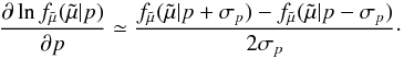$\frac{\mathit{\partial }\ln {\mathit{f}}_{\begin{array}{}\mathrm{˜}\\ \mathit{\mu }\end{array}}\mathrm{\left(}\begin{array}{}\mathrm{˜}\\ \mathit{\mu }\end{array}\mathrm{\right|}\mathit{p}\mathrm{)}}{\mathit{\partial p}}\mathrm{\simeq }\frac{{\mathit{f}}_{\begin{array}{}\mathrm{˜}\\ \mathit{\mu }\end{array}}\mathrm{\left(}\begin{array}{}\mathrm{˜}\\ \mathit{\mu }\end{array}\mathrm{\right|}\mathit{p}\mathrm{+}{\mathit{\sigma }}_{\mathit{p}}\mathrm{)}\mathrm{-}{\mathit{f}}_{\begin{array}{}\mathrm{˜}\\ \mathit{\mu }\end{array}}\mathrm{(}\begin{array}{}\mathrm{˜}\\ \mathit{\mu }\end{array}\mathrm{|}\mathit{p}\mathrm{-}{\mathit{\sigma }}_{\mathit{p}}\mathrm{)}}{\mathrm{2}{\mathit{\sigma }}_{\mathit{p}}}\mathrm{·}$(18)Using a step size of  ± σ_p is logical as we are looking for solutions typically within one standard deviation of the observed value.

4. Testing on synthetic and real samples

We test our method (ML) together with the projection method (PM) as described by Dehnen & Binney (1998) on two types of samples. The first type is a synthetic sample, where nearby “stars” with known mean velocity and velocity dispersion have been generated. This sample allows us to investigate the bias of the two methods. The second type is a sample of real stars taken from the Geneva–Copenhagen survey of nearby F and G dwarfs (Nordström et al. 2004). These stars have measured radial velocities which allow us to estimate their mean velocity and velocity dispersion directly from Eq. (3). We use the resulting estimates as the “true” values when comparing the methods.

4.1. Synthetic samples

4.1.1. Generating the data

The generation of synthetic stars strictly follows the probabilistic model outlined in Sect. 3.1. Observational uncertainties were set to σ_μ = 1, 3, 10 and 30 mas yr^-1 for the components of the proper motions, and to σ_p = 1 mas for the parallaxes. The stars have randomly generated positions (x,y,z) (in pc) within a radius of 100 pc from the sun. Each star is also given a randomized velocity using a normal distribution with the mean parameter  km s^-1 and dispersion matrix D = diag(22²,   14²,   10²) km² s^-2. From the rectangular coordinates the galactic longitude l and galactic latitude b are obtained with $\mathit{l}\mathrm{=}\mathrm{atan}\mathrm{2}\mathrm{\left(}\mathit{y,x}\mathrm{\right)}\hspace{0.17em}\mathit{,} \mathit{b}\mathrm{=}\mathrm{atan}\mathrm{2}\left(\mathit{z,}\sqrt{{\mathit{x}}^{\mathrm{2}}\mathrm{+}{\mathit{y}}^{\mathrm{2}}}\right)\mathit{.}$(19)Then for any position in sky (l,b) we define three orthogonal unit vectors ${u}\mathrm{=}\left[\begin{array}{c}\\ \cos \mathit{b}\cos \mathit{l}\\ \cos \mathit{b}\sin \mathit{l}\\ \sin \mathit{b}\end{array}\right] {l}\mathrm{=}\left[\begin{array}{c}\\ \mathrm{-}\sin \mathit{l}\\ \cos \mathit{l}\\ \mathrm{0}\end{array}\right] {b}\mathrm{=}\left[\begin{array}{c}\\ \mathrm{-}\sin \mathit{b}\cos \mathit{l}\\ \mathrm{-}\sin \mathit{b}\sin \mathit{l}\\ \cos \mathit{b}\end{array}\right]\mathit{,}$(20)where u is the direction towards the star, and l and b are unit vectors in the tangential plane in the sky:  + l in the direction of increasing longitude, and  + b in the direction of increasing latitude.  [u,l,b]  is called the normal galactic triad at the point (l,b).

The true parallax is given by $\mathit{p}\mathrm{=}\frac{\mathrm{1000} \mathrm{mas}}{\sqrt{{\mathit{x}}^{\mathrm{2}}\mathrm{+}{\mathit{y}}^{\mathrm{2}}\mathrm{+}{\mathit{z}}^{\mathrm{2}}}}\mathit{,}$(21)whereupon the true proper motion in longitude and latitude is calculated as ${\mathit{\mu }}_{\mathit{l}}\mathrm{=}\frac{\mathit{p}}{\mathit{K}}\hspace{0.17em}{l}\mathrm{·}{v} \mathrm{and} {\mathit{\mu }}_{\mathit{b}}\mathrm{=}\frac{\mathit{p}}{\mathit{K}}\hspace{0.17em}{b}\mathrm{·}{v}$(22)respectively. Here, K = 4.7405 km s^-1 kpc^-1 (mas yr^-1)^-1 is the numerical constant relating mas yr^-1 to km s^-1 kpc^-1.

To get the observed proper motions and parallax, the errors in proper motion and parallax are added to the true values. Errors were drawn from the normal distribution with zero mean value and standard deviation equal to the observational uncertainties σ_μ and σ_p.

As the simulated data set depends on many different parameters it is not possible to investigate the methods for all possible combination of the parameters. We restrict ourselves to keep most of the parameters fixed (, D, R and σ_p), and only study how the methods perform as a function of n, the number of stars in the sample, and σ_μ, the uncertainty in proper motion. We use n = 30, 100, 300, 1000 and σ_μ = 1, 3, 10, 30 mas yr^-1, which gives 16 different combinations. For each combination 100 samples are generated with different seeds for the random generator. The 100 samples are thus different in the generated true positions and velocities, as well as in the observational errors. The PM and ML methods were applied to all 1600 samples and the mean values and RMS variations of the estimated parameters calculated.

4.1.2. Results

With the synthetic sample we can see a difference in how the uncertainty in proper motion affects the values of the calculated velocities and velocity dispersions for the two methods.

In the left column of Fig. 1, results from the PM are shown. As expected, the dispersions are increasingly biased towards higher values when the uncertainty in proper motion increases. The effect is negligible when σ_μ = 1 or 3 mas yr^-1, but for σ_μ = 10 or 30 mas yr^-1 the increase in the dispersions is quite significant. This is reasonable since an error of 30 mas yr^-1, at the median distance of the sample (80 pc), corresponds to a linear velocity error of about 11 km s^-1, which is comparable to the true velocity dispersion. As can be seen in the bottom left panel of Fig. 1, the dispersion component in w is most severely overestimated ( ≃ 15 km s^-1 versus the true value 10 km s^-1), while the v and u components are somewhat less affected (18 versus 14 km s^-1 and 25 versus 22 km s^-1, respectively). Indeed, in all the cases the estimated dispersion (for n ≥ 100) is roughly equal to the sum in quadrature of the true dispersion and the linear velocity error corresponding to the proper motion uncertainty. This is a useful rule-of-thumb to estimate the expected bias of the PM under more general conditions. A more unexpected result is that, for the smallest samples (n = 30), the resulting dispersion matrix is unphysical (not positive definite) in about 1% of the cases. However, this does not happen with the larger samples.

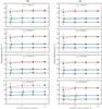Fig. 1 Plots illustrating velocity dispersion versus the number of stars, for different values of σμ, as calculated for the synthetic samples described in Sect. 4.1. Diagrams in the left column are for the projection method (PM), the right column is for the maximum likelihood method (ML). The symbols represent the different galactic components of the dispersion: σu (•), σv (▾), σw (▴). The true values are indicated by the horizontal lines.

The column to the right in Fig. 1 show the results of the ML method. We note that:

• 1.

  Unlike the PM, the ML method is able to give unbiaseddispersions even for very large σ_μ, at least if the sample is not too small (n ≥ 100).

• 2.

  For the smallest samples (n = 30) it is often necessary to use regularization. In most of these cases it is sufficient to use α = 0.5, which does not change the axis ratio much. Only in very few cases was α > 3 needed, which gives a nearly isotropic dispersion.

For the smallest sample size both PM and ML tend to underestimate the dispersion, especially along the major axis (u component) of the velocity ellipsoid.

4.2. Application to the Geneva-Copenhagen survey

The Geneva-Copenhagen survey (Nordström et al. 2004) is the largest and most complete study of a magnitude-limited, kinematically unbiased sample of F and G stars in the solar neighbourhood. It contains space velocities, Strömgren photometry, metallicities, rotation velocities and ages for more than 16 000 stars. The catalogue gives complete (u,v,w) space velocities based on Hipparcos data and radial velocities, from which the “true” vales of the mean velocity and velocity dispersion can be computed using Eq. (3).

4.2.1. Data used

Not all stars in the Geneva–Copenhagen survey could be used in this study. Stars with large relative parallax errors (p/σ_p < 10), large peculiar tangential velocities (|Δτ |  > 200 km s^-1), or missing some of the necessary data were eliminated. The remaining 7796 stars were divided into 10 bins of approximately equal size, sorted by their Strömgren color index b − y.

4.2.2. Results

Table 2 and Fig. 2 give results of both estimation methods (PM and ML) using tangential velocities only, as well as from the full space velocities (GC). No error bars are given here as the computation of the formal errors has not been implemented (cf. Sect. 5). It is seen that PM and ML give very similar results for all the samples and for all nine kinematic parameters, and they both agree well with the “true” values (GC). In the light of the experiments with the synthetic samples this is not surprising since the observational errors in this case are generally small (few mas), resulting in almost negligible tangential velocity errors. However, it is gratifying to note that the ML performs at least as well as the PM in this case.

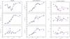Fig. 2 Left: mean velocities versus color index b − y for stars in the Geneva-Copenhagen (GC) survey. Middle: velocity dispersions σu,σv,σw versus color index b − y for stars in the GC survey. Right: correlation coefficients ρij = Dij(DiDjj) − 1/2 (where i,j = u,v,w) from the estimated dispersion matrix versus color index b − y for stars in the GC survey. Values calculated directly from the GC data are shown as a solid line. The symbols represent the two different methods used: PM (°), ML (•).

5. Conclusions

Galactic astrophysics is entering a new era in which large-scale astrometric, photometric and spectroscopic surveys provide vast quantities of data that need to be interpreted in terms of different structural, kinematic and evolutionary models. In this context it is essential to have at our disposal estimation techniques that can deal with incomplete data (e.g., missing radial velocities) and that are statistically efficient and reasonably unbiassed. It is also important to take the observational uncertainties into account, for although some of the surveys are much more precise than earlier ones (e.g., Gaia versus Hipparcos), they are also applied to much more distant stars, making the observational errors no less important.

For many stars brighter than 17th magnitude Gaia will provide the complete space velocity vector through a combination of its astrometric and spectroscopic measurements. However, the vast majority of stars observed by Gaia are fainter than 17th magnitude and will have no radial velocities. This is also the magnitude range where the astrometric errors in parallax and proper motion start to become problematic for studies of the galactic kinematics beyond the solar neighbourhood. For example, solar-type stars at 5 kpc distance will be observed at apparent magnitude 18 to 20, depending on the extinction, resulting in relative parallax errors of at least 50% and transverse velocity errors of several km s^-1. The very large number of such stars will permit a detailed mapping of their distribution functions provided that the statistical biases can be mastered.

In this paper we have considered a seemingly very simple problem, namely to estimate the nine parameters describing the velocity distribution of stars under the Schwarzschild approximation, based exclusively on astrometric data and taking into account the observational uncertainities in the parallaxes and proper motions. The rigorous application of the maximum likelihood method to this problem turns out to be surprisingly complex, and we have devised an approximate numerical method to solve it. We have tested the method on both synthetic and real samples of stellar data, and found that it performs slightly better than the simple projection method (Dehnen & Binney 1998), especially when the observational errors are important and for small samples. For very small samples (less than about 30 stars) the projection method sometimes gives unphysical results. This is avoided with our method, which however may require regularization for such small samples, leading to a more isotropic dispersion tensor.

Several authors have applied maximum likelihood or Bayesian methods to estimate stellar kinematics using formulations that differ in various aspects from our approach. For example, Dehnen (1998) describes how general three-dimensional velocity distributions can be derived from tangential velocities, using the so-called maximum penalized likelihood estimate, i.e., a maximum-likelihood estimate constrained to give a smooth velocity distribution. While this method is very general, it does not take into account the observational uncertainties. Hogg et al. (2005) and Bovy et al. (2009) derive the parameters for a mixture of Gaussian distributions from tangential velocity data. While they do include the observational uncertainties through a linear propagation to the tangential velocities, their formalism is quite different from ours in the treatment of the parallax errors. It could be interesting to compare the two methods as they both depend on (different) approximations for small relative parallax errors.

The present method could be extended and generalized in various ways. One obvious extension is to allow that some stars have a measured radial velocity instead of, or in addition to the astrometric data. Another is to consider a more complex velocity distribution, e.g., a superposition of several Gaussian components. It is also desirable to apply a more efficient numerical solution technique than the downhill simplex method which was chosen for the present experiments for its ease of implementation. Alternative methods such as a quasi-Newton with finite differences (Press et al. 2007) would almost certainly be much more efficient. We note that the computing time scales linearly with the number of stars (for a fixed number of kinematical parameters), which makes it feasible to apply the ML method also to much larger samples than in our experiments. Finally, the formal errors (or more generally confidence regions) of the estimated quantities need to be computed, which could be done with moderate effort by mapping the log-likelihood function around its maximum.

Acknowledgments

We wish to thank the anonymous referee for several useful suggestions which helped to improve the manuscript.

References

All Tables

All Figures

Fig. 1 Plots illustrating velocity dispersion versus the number of stars, for different values of σμ, as calculated for the synthetic samples described in Sect. 4.1. Diagrams in the left column are for the projection method (PM), the right column is for the maximum likelihood method (ML). The symbols represent the different galactic components of the dispersion: σu (•), σv (▾), σw (▴). The true values are indicated by the horizontal lines.

In the text

Fig. 2 Left: mean velocities versus color index b − y for stars in the Geneva-Copenhagen (GC) survey. Middle: velocity dispersions σu,σv,σw versus color index b − y for stars in the GC survey. Right: correlation coefficients ρij = Dij(DiDjj) − 1/2 (where i,j = u,v,w) from the estimated dispersion matrix versus color index b − y for stars in the GC survey. Values calculated directly from the GC data are shown as a solid line. The symbols represent the two different methods used: PM (°), ML (•).

In the text

References

- Aumer, M., & Binney, J. J. 2009, MNRAS, 397, 1286 [NASA ADS] [CrossRef] [Google Scholar]
- Binney, J. J., Dehnen, W., Houk, N., Murray, C. A., & Penston, M. J. 1997, in Hipparcos – Venice ’97, eds. R. M. Bonnet, E. Høg, P. L. Bernacca, L. Emiliani, A. Blaauw, C. Turon, J. Kovalevsky, L. Lindegren, H. Hassan, M. Bouffard, B. Strim, D. Heger, M. A. C. Perryman, & L. Woltjer, ESA Spec. Publ., 402, 473 [Google Scholar]
- Bovy, J., Hogg, D. W., & Roweis, S. T. 2009, ApJ, 700, 1794 [NASA ADS] [CrossRef] [Google Scholar]
- Brosche, P., Schwan, H., & Schwarz, O. 2001, Astron. Nachr., 322, 15 [Google Scholar]
- de Bruijne, J. H. J. 2012, Ap&SS, 341, 31 [NASA ADS] [CrossRef] [Google Scholar]
- Dehnen, W. 1998, AJ, 115, 2384 [NASA ADS] [CrossRef] [Google Scholar]
- Dehnen, W., & Binney, J. J. 1998, MNRAS, 298, 387 [NASA ADS] [CrossRef] [Google Scholar]
- ESA. 1997, The Hipparcos and Tycho Catalogues, ESA SP-1200 [Google Scholar]
- Hogg, D. W., Blanton, M. R., Roweis, S. T., & Johnston, K. V. 2005, ApJ, 629, 268 [NASA ADS] [CrossRef] [Google Scholar]
- Lagarias, J. C., Reeds, J. A., Wright, M. H., & Wright, P. E. 1998, SIAM J. Optimizat., 9, 112 [Google Scholar]
- Mignard, F. 2000, A&A, 354, 522 [NASA ADS] [Google Scholar]
- Nordström, B., Mayor, M., Andersen, J., et al. 2004, A&A, 418, 989 [NASA ADS] [CrossRef] [EDP Sciences] [Google Scholar]
- Press, W., Teukolsky, S., Vetterling, W., & Flannery, B. 2007, Numerical Recipes: The Art of Scientific Computing, 3rd edn. (Cambridge University Press) [Google Scholar]
- Steinmetz, M., Zwitter, T., Siebert, A., et al. 2006, AJ, 132, 1645 [NASA ADS] [CrossRef] [Google Scholar]
- van Leeuwen, F. 2007, A&A, 474, 653 [NASA ADS] [CrossRef] [EDP Sciences] [Google Scholar]
All Tables
An example with 100 stars illustrating how the estimated velocity dispersion depends on the value of α.
Results of both the projection method (PM) and our maximum likelihood method (ML) applied to samples from the Geneva-Copenhagen survey (Nordström et al. 2004).