| Issue |
A&A
Volume 551, March 2013
|
|
|---|---|---|
| Article Number | A14 | |
| Number of page(s) | 10 | |
| Section | Stellar atmospheres | |
| DOI | https://doi.org/10.1051/0004-6361/201220425 | |
| Published online | 12 February 2013 | |
Fundamental parameters of bright Ap stars from wide-range energy distributions and advanced atmospheric models
1
Institute of Astrophysics, Georg-August University,
Friedrich-Hund-Platz 1,
37077
Göttingen,
Germany
e-mail: This email address is being protected from spambots. You need JavaScript enabled to view it.
2
Institute of Astronomy, Russian Academy of Science,
Pyatnitskaya 48,
119017
Moscow,
Russia
3
Universität Wien, Institut für Astronomie,
Türkenschanzstraße
17, 1180
Wien,
Austria
4
Department of Physics and Astronomy, Uppsala
University, PO Box
516, 751 20
Uppsala,
Sweden
Received: 21 September 2012
Accepted: 8 November 2012
Abstract
Aims. As a well-established procedure for the vast majority of normal main-sequence stars, determination of atmospheric and stellar parameters turns to be a challenging process in case of magnetic chemically peculiar stars. Inhomogeneous distribution of chemical elements and strong magnetic fields make most of the standard photometric and spectroscopic calibrations inapplicable for this class of stars. In this work we make use of available observed energy distributions calibrated to absolute units, stellar parallaxes, high-resolution spectroscopic observations, and advanced stellar atmosphere models to derive parameters of three bright Ap stars: 33 Lib, γ Equ, and β CrB.
Methods. Model atmospheres and fluxes were computed with the LLmodels code. Synth3 and Synthmag codes were used to compute profiles of individual spectral lines involved in abundance analysis.
Results. For each of the stars, we construct a self-consistent atmospheric models assuming normal and depleted helium compositions and derive empirically stratification profiles of certain elements. The effective temperatures and surface gravities are found from the simultaneous fit to spectroscopic, photometric, and spectrophotometric observations calibrated to absolute units. We show that using advanced model atmospheres and accurate stellar parallaxes allows one to derive stellar radii with high accuracy, and these are consistent with those obtained from independent but more complicated interferometric observations.
Key words: stars: chemically peculiar / stars: atmospheres / stars: abundances / stars: fundamental parameters / stars: general
© ESO, 2013
1. Introduction
Accurate knowledge of fundamental stellar (mass, radius, luminosity, metallicity, age) and atmospheric (effective temperature, surface gravity, atmospheric abundances) parameters is essential for many fields of modern astrophysics. Stellar masses and abundances determine the whole chain of stellar evolution stages of a single star, and obtaining stellar luminosities and radii by means of observed data allows one to determine ages of stars, as well as to derive other parameters of interest, such as atmospheric chemistry from spectroscopic observations, to characterize extrasolar planets from transit data, to carry out asteroseismic modeling, and much more.
Determining stellar parameters is a delicate process, even in the case of normal stars, because it relies on theoretical evolutionary and atmospheric models. The former requires knowing metallicities and masses, the latter also needs effective temperatures and gravities as input. These are usually obtained from spectroscopic and photometric data employing well-developed calibration schemes. For chemically peculiar (CP) stars, however, things get much more complicated mainly because of the abnormal chemical composition of their atmospheres (see, e.g., Ryabchikova et al. 2004). This makes the spectra and energy distributions of CP stars look very different from their normal analogs, and therefore most of the photometric calibrations simply fail to work for CP stars. Furthermore, the strong surface magnetic fields detected in many CP stars additionally complicate the analysis of their spectra and determination of atmospheric parameters.
Since all parameters are linked, the accuracy in derived parameters, such as Teff and log (g), must be as high as possible. This is why the full set of stellar and atmospheric parameters can ideally only be derived using an iterative procedure where each parameter is adjusted in such a way as to fit all available observed data. Then, if needed, the other parameters are recalculated accordingly. For instance, deriving Teff and log (g) from photometric data and employing relevant calibrations one can carry out a detailed abundance analysis based on model atmospheres, but if derived abundances turn out to be different from those assumed in the construction of the model atmospheres then the latter must be recalculated with the appropriate chemistry, and the whole process should be repeated again. Because of the lack of appropriate calibrations and the wide diversity of abundance patterns, this is the only robust scheme for analyzing CP stars (see, e.g., Kochukhov et al. 2009; Shulyak et al. 2009; Pandey et al. 2011).
Recently, interferometry has been successfully applied to CP stars resulting in a first estimate of the radii of three stars: α Cir (HD 128898, Bruntt et al. 2008), β CrB (HD 137909, Bruntt et al. 2010), and γ Equ (HD 201601, Perraut et al. 2011). No doubt interferometry is a powerful technique with the strong advantage of providing model-independent estimates of stellar sizes, but its current world-wide facilities, unfortunately, are limited only to bright stars.
In this work we apply a self-consistent atmospheric analysis to three well-known magnetic CP stars: β CrB (HD 137909), γ Equ (HD 201601), and 33 Lib (HD 137949). Collecting available photometric, spectrophotometric, and spectroscopic observations we perform detailed abundance and stratification analysis of a number of chemical elements in the atmosphere of each star. The effective temperatures and gravities are found iteratively by comparing theoretical fits to all available observables. Using fluxes calculated consistently with model atmospheres, available stellar parallaxes, and observed fluxes calibrated to absolute units, we derive stellar radii and compare them with interferometric results.
2. Observations
Our investigation is based mainly on the low-resolution spectroscopic observations calibrated to absolute units and obtained by Space Telescope Imaging Spectrograph (STIS)1 mounted at the Hubble Space Telescope. STIS provides wide wavelength coverage (λλ1700−10 200) that is excellent for accurate analysis of the energy distributions of early type stars where both UV and visual fluxes are highly important. Among our targets, only 33 Lib was not observed with STIS. Nevertheless, medium-band spectro-photometric observations by Adelman et al. (1989) are available for all objects, as are UV fluxes from the International Ultraviolet Explorer (IUE)2. For 33 Lib and β CrB, additional wide-band UV fluxes were taken from the TD1 space mission (Boksenberg et al. 1973; Thompson et al. 1978). For β CrB we also made use of the spectro-photometric measurements of Alekseeva et al. (1996), Breger (1976), Komarov et al. (1995), and UV low-resolution fluxes from the Astron space satellite (Boiarchuk 1986).
We note that CP stars are known to demonstrate photometric variability, most of which is caused by the inhomogeneous surface distribution of chemical elements. However, as can be seen from e.g. Shulyak et al. (2010a) and Krtička et al. (2012), the amplitude of this variability is rather small to influence the derived effective temperatures much. For instance, using Adelman’s spectrophotometric catalog, we find that the relative characteristic correction to the effective temperatures due to flux variability is only a few ten K’s for all three target stars. Because of this, and also because the datasets listed above are not homogeneous in the sense of observing times and number of observations performed, we used mean fluxes when possible. For instance, only phase-averaged fluxes were used from Adelman’s catalog and the IUE data archive.
Chemical abundance and stratification analysis was based on high-resolution, high signal-to-noise-ratio spectra obtained with the UVES instrument (Dekker et al. 2000) at the ESO VLT. Observations of 33 Lib and β CrB were carried out in the context of program 68.D-0254, and published by, e.g., Ryabchikova et al. (2008), while spectra of γ Equ were extracted from the ESO archive (program 76.D-0169). Spectra of all three stars were obtained using both dichroic modes, thus covering wavelength intervals from λ3030 to λ10400 with a few gaps. Spectral resolution is about 80 000, and the signal-to-noise ratio at λ5000 is about 300–400. A detailed description of the data reduction is given by Ryabchikova et al. (2008; 33 Lib and β CrB) and by Cowley et al. (2007; γ Equ). In addition, for 33 Lib and γ Equ we used the UVES slicer spectra covering the λλ4960−6990 region and providing a resolving power of λ/Δλ ≈ 115 000. Time-resolved observation of these stars were obtained in the context of ESO programs 72.D-0138 and 077.D-0150 (e.g. Kurtz et al. 2006). We used average spectra constructed from the total of 111 and 178 short exposures for 33 Lib and γ Equ, respectively. Reduction of these data followed procedures described by Ryabchikova et al. (2007).
In the course of our analysis we found that for the β CrB and γ Equ the Hβ line of the UVES spectra always require systematically different temperatures compared to the one derived from the spectral energy distribution (SED) and other hydrogen lines. We attribute this to a problem of continuum normalization and made use of additional observations from different instruments. In particular, for β CrB we used spectroscopic data obtained at 2.6-m telescope mounted at Crimean Astrophysical Observatory (CrAO, Savanov & Kochukhov 1998). For γ Equ we used medium resolution spectra (R ≈ 37 000) obtained with the echelle spectrograph GIRAFFE, mounted at the 1.9-m Radcliffe telescope of SAAO (South African Astronomical Observatory). The data reduction of the GIRAFFE spectra was based on Vienna automatic pipeline for echelle spectra processing described in Tsymbal et al. (2003).
3. Basic methods
3.1. Model atmospheres
Our approach is based on the models and synthetic fluxes computed with the LLmodels stellar model atmosphere code (Shulyak et al. 2004). The code can treat individual homogeneous and depth-dependent abundances, which is a key feature in our modeling. In addition, the effect of the magnetic field is fully accounted via detailed computations of the anomalous Zeeman splitting and polarized radiative transfer as described in Khan & Shulyak (2006a). In all calculations we adopted magnetic field vector to lay perpendicular to the normal of the stellar surface (see Khan & Shulyak 2006b, for more details). This makes LLmodels a powerful tool for the modeling of the observed characteristics of magnetic CP stars. The model fluxes are computed on a fine frequency grid with the highest point density at the wavelengths occupying the region of maximum stellar flux. A total of about 600 000 frequency points are usually used, which provides the necessary resolution for accurate computation of photometric indicies of broad- and narrow-band photometric systems. Lines opacity coefficient is computed based on atomic parameters extracted from the VALD database (Piskunov et al. 1995; Kupka et al. 1999), which presently includes more than 6.6 × 10⁷ atomic lines. Most of them come from the latest theoretical calculations performed by R. Kurucz3.
Because of their large overabundance in atmospheres of Ap stars, rare-earth elements (REE) play an important and sometimes even dominating role in the appearance of spectroscopic features (Mashonkina et al. 2009, 2005) and can also affect the SED (Shulyak et al. 2010b). Here we used the same line lists of REE elements as presented in Shulyak et al. (2010b). The studies by Mashonkina et al. (2009, 2005) demonstrate that the line formation of Pr and Nd can strongly deviate from the local thermodynamic equilibrium (LTE) with the doubly ionized lines of these elements are unusually strong due to the combined effects of stratification of these elements and departures from LTE (known among spectroscopists as the “REE anomaly”). However, a precise NLTE analysis is beyond the scope of this paper and currently could not be directly coupled to a model atmosphere calculation. Therefore, we followed the approach outlined in Shulyak et al. (2009) where the authors used a simplified treatment of the REE NLTE opacity by reducing the oscillator strengths for the singly ionized REE lines by the corresponding LTE abundance difference, while using the abundances derived from second ions as input for model atmosphere calculations (or vice versa). Applying this line scaling procedure allowed us to mimic the line strengths that correspond to the NLTE ionization equilibrium abundance for each REE.
3.2. Abundance and stratification analysis
Initial homogeneous abundances for model calculations were taken from the papers by Ryabchikova et al. (2004; 33 Lib and β CrB) and by Ryabchikova et al. (1997) for γ Equ. These abundances were slightly corrected with synthetic spectral synthesis taking into account rather large magnetic fields of the program stars. Spectrum synthesis was performed by the magnetic synthesis code SYNTMAG (see Kochukhov 2007) using extraction of the atomic parameters and Landé-factors from the VALD database. To make abundance analysis of magnetic stars more efficient, we used the equivalent width method with the newly developed code WidSyn. This program provides an interface to the SYNTMAG code and allows abundances to be derived using theoretical equivalent widths obtained from the full polarized radiative transfer spectrum synthesis. This improved equivalent width method considerably accelerates abundance analysis without sacrificing accuracy.
The stratification of chemical elements was modeled by employing the DDAFit IDL-based automatic procedure that finds chemical abundance gradients from the observed spectra (see Kochukhov 2007). In this routine, the vertical abundance distribution of an element is described with the four parameters: chemical abundance in the upper atmosphere, abundance in deep layers, the vertical position of abundance step, and the width of the transition region where chemical abundance changes between the two values. All four parameters can be modified simultaneously with the least-squares fitting procedure and based on observations of an unlimited number of spectral regions. This procedure was successfully employed by a number of element stratification studies (e.g., Ryabchikova et al. 2005; Kochukhov et al. 2009; Shulyak et al. 2009; Pandey et al. 2011).
For Pr and Nd in γ Equ, we performed an NLTE stratification analysis as described in Mashonkina et al. (2005, 2009) using a trial-and-error method and the observed equivalent widths of the lines of the first and second ions. In NLTE calculations magnetic field effects were roughly approximated by pseudomicroturbulent velocity individual for each line. Such an analysis is applicable only for stars with small or moderate magnetic fields, e.g. for HD 24712, γ Equ (Mashonkina et al. 2005, 2009).
3.3. Determination of fundamental parameters
We follow the basic steps of the iterative procedure of atmospheric parameters determination outlined in, e.g., Shulyak et al. (2009). Briefly, this procedure consists of repeated steps of stratification and abundance analysis that provide an input for the calculations of model atmosphere until atmospheric parameters (Teff, log (g), etc.) converge and theoretical observables (energy distribution, profiles of hydrogen lines, etc.) fit observations. Thus, the derived abundance pattern is consistent with the physical parameters of the final stellar atmosphere.
We used low-resolution spectroscopic and/or spectro-photometric data calibrated to absolute units and available stellar parallaxes to derive radii of investigated stars. Fitting the full energy spectrum makes it possible to find reliable values for the atmospheric log (g) by matching the amplitudes of Balmer jump, which is very difficult or even impossible to do when only spectroscopic indicators or photometric indices are used. The fit to observed energy distributions is carried out on each iteration of abundance analysis using a grid of model atmospheres computed for a set of [Teff, log (g)] values. The radii of the star is found by minimizing the deviations between observed and predicted absolutely calibrated fluxes.
However, one important uncertainty remains in this analysis. As follows from the computations of atomic diffusion, helium always sinks in subphotosheric layers of A-F stars (Michaud et al. 1979). The same He depletion is also found by the diffusion models of the optically thin layers (Leblanc & Monin 2004), suggesting that the atmospheres of CP stars of spectral types A-F may well be He-deficient. No suitable diagnostic He lines are available for cool Ap stars to verify this conclusion observationally. The question of whether helium is indeed removed from the atmosphere is particularly important because this may noticeably change the molecular weight and T-P stratification of He-weak models in deep layers where temperatures become high enough for He to contribute to the total opacity coefficient. Having no clues to the true He stratification, we thus consider an additional case of He-weak atmosphere with adopted He abundance of [He/H] = −4 (decreasing He abundance below this value has only a marginal or no effect).
Fudamental parameters of Ap stars.
4. Results
In this section we present the results of the parameter determinations for individual Ap stars, which are combined in Table 1. For completeness, this table also lists our previous results derived for a few additional CP stars using the same analysis methodology. We also find that, with a few exceptions, the application of realistic model atmospheres did not result in a significant change of the mean element abundance estimates with respect to the studies cited above. Therefore, in the following we focus on the analysis of the vertical abundance profiles.
4.1. β CrB (HD 137909)
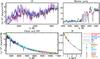 |
Fig. 1 Observed and predicted energy distributions of β CrB for two best-fitted models with solar and depleted helium contents. |
Among the three targets, β CrB is probably the most studied one. A number of independent spectrophotometric observations of energy distributions make it possible to test predictions of atmospheric models, as well as estimate uncertainties of derived fundamental parameters in detail. Furthermore, β CrB is known to be a binary system with orbital elements presented by Tokovinin (1984) and North et al. (1998). More recently, Bruntt et al. (2010) have carried out interferometric observations of the system, which resulted in the first model-independent determination of the radii of primary (A) and secondary (B) components: R(A) = 2.63 ± 0.09 R⊙, R(B) = 1.56 ± 0.07 R⊙. However, authors still used scaled-solar models computed with ATLAS9 model atmosphere code (Kurucz 1992, 1993) to predict bolometric flux of the system and thus to derive effective temperatures for both components. This was necessary because all modern flux data always contain the combined light of the two components. This is also true for the STIS observation, which was done with the 0.2′′ slit width on 25 Aug. 2003 when the visible separation between system components was r < 0.1′′. Effective temperatures were found to be Teff(A) = 7980 ± 180 K and Teff(B) = 6750 ± 230 K, respectively. The secondary component thus provides an important ≈18% contribution to the bolometric flux of the system and thus has been taken into account in our SED fitting procedure.
Available spectra of β CrB made it possible to analyze the stratification of five chemical elements: Mg, Si, Ca, Cr, and Fe, using from 8 to 23 neutral and singly-ionized lines per element. We did not perform NLTE Pr-Nd stratification analysis because of a rather strong magnetic field and an absence of any significant Pr-Nd anomaly (Ryabchikova et al. 2004), which is a manifestation of the rare-earth stratification. Starting from the Teff = 8000 K, log (g) = 4.3 homogeneous abundance model, and abundances presented in Ryabchikova et al. (2004), the atmospheric parameters were iterated to match the observed SED and profiles of hydrogen lines. All model atmospheres were computed with ⟨ Bs ⟩ = 5.4 kG surface magnetic field (Ryabchikova et al. 2008). The best fitted parameter of the primary fall in the range 8000 < Teff(A) < 8050 K, 3.9 < log (g)(A) < 4.0 and the respective fits to the SED and hydrogen lines are shown in Figs. 1 and 2. Generally, the Teff of the star is constrained by the slope of the Paschen continuum and hydrogen lines, while the log (g) is best controlled by the amplitude of the Balmer jump. We find that the contribution of the β CrB-B is crucial for the Paschen continuum and IR region, and when ignoring it we were not able to obtain a consistent fit to SED and H-lines with any set of atmospheric parameters.
From Fig. 1 it is clear that there is a systematic difference between space and ground-based observations. The STIS, IUE, TD1, and Astron data agree very well in the UV region below λ2900. At the same time, STIS provides less flux in the visual and NIR than all ground-based photometric and spectrophotometric observations, which in turn agree fairly well with each other, with the exception of NIR (where some deviation can be seen, especially in the case of data from the Odessa catalog) and λλ3800−5000 region. Most likely this is due to the different calibration methods applied to the observed data, and it is hard to give a preference to any of these datasets. Because STIS provides most homogeneous sets of observations covering a wide wavelength range from UV to NIR, we used it as a reference in the model-fitting process.
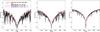 |
Fig. 2 Observed and predicted profiles of hydrogen lines of β CrB. Full line – He norm model; dashed line – He-weak model. |
Two problems still remain. First, none of the models can reasonably fit the UV spectrum of the star below λ2500. The secondary component is too faint to influence the combined flux in this spectral region. Because all UV data agree well with each other, we are inclined to conclude that this discrepancy between theoretical and observed fluxes is due to missing opacity in our models. The second problem arises from the fit to H-lines. Only Hα and Hβ are fit satisfactory. The computed profiles of Hγ are always wider than the observed ones even for He-weak model with lower Teff = 8050 K that demonstrate somewhat better agreement for these two particular lines and worse for Hα. By increasing Teff of the secondary within the limits given by Bruntt et al. (2010), one can obtain a slightly lower Teff for the primary and thus narrower profiles of Hγ, respectively, but the fit to both NIR fluxes and particularly Hα profile then becomes noticeably worse. By integrating STIS fluxes and theoretical fluxes of the A = [8050,4.0,2.50 ± 0.07] , B = [6750,4.2,1.56] model, we estimated a corresponding uncertainty in the effective temperature due to a difference between observed and predicted fluxes to be ΔTeff = 50 K. This means that the true Teff of β CrB is probably slightly overestimated in our analysis. On the other hand, an uncertainty in He abundance results in a similar 50 K error, thus accounting for both, these effects could lower a temperature of the star by 100 K compared to the temperature derived in this study.
The final adopted parameters are (component = [Teff(K), log (g)(dex),R(R⊙)] ): A = [8050,4.0,2.50 ± 0.07] for the He-weak model and A = [8100,3.9,2.47 ± 0.07 for the He-normal (e.g., with solar helium composition) model. The parameters of the secondary were taken from Bruntt et al. (2010): B = [6750,4.2,1.56] . We used the Hipparcos parallax of π = 28.60 ± 0.69 mas from van Leeuwen (2007). The errors of the derived radii results from the stellar parallax uncertainty.
Using ground-based spectrophotometry led to a noticeable increase in the stellar radii. For instance, the fit to the data obtained by Breger (1976) requires A = [8050,4.0,2.70 ± 0.07] for He-weak and A = [8050,3.8,2.65 ± 0.07] for He-norm models, respectively. The differences between STIS and ground-based observations correspond to the non-negligible difference in the derived stellar radii of ΔR ≈ 0.2 R⊙. This reflects certain problems in the applied flux calibration procedures. But in spite of the vertical offset, the shape of SEDs remains practically the same, therefore the effective temperatures derived from the two datasets are very similar.
Figure 3 illustrates stratification profiles derived from the final He-norm and He-weak models. A substantial change in the position of the abundance jump is found for Mg, for which the He-norm model results in its narrowing and deeper position compared to the He-weak model. Elements Ca and Fe demonstrate changes in the abundance amplitude in upper atmospheric layers, but we find that solution for Ca is quite uncertain in the highest layers with estimated errors on the order of ± 1 dex or higher. Stratifications of Si and Cr stay almost unchanged, with Si accumulating at much deeper photospheric layers than what was found for other elements. The changes in stratification profiles observed in Fig. 3 are a combined effect of decreasing He content and Teff by 50 K, i.e. not entirely due to He content. The effect of decreasing He abundance manifests itself in the increased log (g) by 0.1 dex needed to fit the SED of the star. Thus, accounting for a possible peculiar He content does have a well determined effect on the stellar parameter determination, and we suggest to compute models with strongly deficient He content (i.e. in the same way it is done in this research) when analyzing cool CP stars where true He abundance cannot be derived spectroscopically.
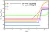 |
Fig. 3 Depth-dependent distribution profiles of chemical elements in the atmosphere of β CrB. |
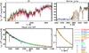 |
Fig. 4 Observed and predicted energy distributions of γ Equ for two best-fitted models with solar and depleted helium contents. |
4.2. γ Equ (HD 201601)
Another well known roAp star with a rich spectrophotometric dataset available is γ Equ. Similar to β CrB, recent interferometric observations by Perraut et al. (2011) provide a radius of the star R = 2.20 ± 0.12 R⊙. It is also a binary system (see Fabricius et al. 2002) with γ Equ-B having much cooler temperature (Teff(B) = [4570, 4833] K) and thus smaller radius than β CrB-B, which then translates to the contribution of about 6% to the total flux of the system (Perraut et al. 2011). The authors also estimated the effective temperature of the system Teff(A + B) = 7364 ± 235 K, and thus Teff(A) = 7253 K. This is much cooler than the temperature of Teff = 7700 K adopted for γ Equ in the latest detailed spectroscopic study by Ryabchikova et al. (2002).
Due to extremely sharp spectral lines and weaker magnetic field which minimize the blending effects, γ Equ provides a possibility to perform a stratification analysis for 18 chemical elements: Na, Mg, Si, Ca, Sc, Ti, V, Cr, Mn, Fe, Co, Ni, Sr, Y, Zr, Ba, Pr, Nd. This represents the most complete empirical study of element diffusion in an atmosphere of a single star to date. Starting from the initial model with Teff = 7700 K, log (g) = 4.2 from Ryabchikova et al. (1997), we iterated stratification analysis and model atmosphere calculations until a minimal deviation between observed spectrophotometric observations and model fluxes was obtained. The surface magnetic field introduced in model atmosphere computations was ⟨ Bs ⟩ = 4 kG. In Sc, V, Mn, Co stratification calculations laboratory data for hyperfine structure (hfs) were taken into account. They were extracted from the following papers: Villemoes et al. (1992; Sc II), Armstrong et al. (2011; V II), Blackwell-Whitehead et al. (2005; Mn I), Holt et al. (1999; Mn II), Pickering (1996; Co I), Bergemann et al. (2010; Co II). Hyperfine structure for Pr ii was also included in the Pr stratification analysis (see Mashonkina et al. 2009) with the hfs-constants from Ginibre (1989). In the case of He-norm setting, we find that models with A = [7600,4.0,2.04 ± 0.05] , B = [4500−4750,4.5,0.65−0.70] provide the best fit to the observed SED applying parallax π = 27.55 ± 0.62 mas from van Leeuwen (2007). Assuming B = [5000,4.5,0.80] results in a higher temperature of the primary A = [7700,4.0,1.95 ± 0.05] . To fit the Balmer lines, however, a lower effective temperatures of about Teff = 7300 K is needed. Therefore, to maintain a satisfactory fit to both Balmer lines and the SED, a slightly cooler A = [7550,4.0,2.07 ± 0.05] was chosen. We note that formally the model with log (g) = 3.8 provides a better fit to SED (χ2 = 1.19) than the model with log (g) = 4.0 (χ2 = 1.40) with a difference visible at the Balmer jump region (top right plot of Fig. 4). But the log (g) = 3.8 then results in too low a mass of the star, M = 0.98 M⊙, which is unreasonable for a main sequence object with Teff = 7550 K. No distinction could be made between these two values of log (g) from hydrogen line profiles because they are insensitive to the atmospheric gravity in this temperature range.
From the SED comparison presented in Fig. 4, it is seen that good agreement between observations and model predictions is obtained for all spectral intervals represented from the UV to IR. Ground-based spectrophotometric data are also found to be consistent with the STIS observations, except observations obtained by the Odessa research group which are systematically lower. The derived effective temperatures from the SED are reasonably close to those of Ryabchikova et al. (1997). This is because in the latter work the authors fitted observations of Adelman et al. (1989), which required Teff = 7700 K to match the slope of the Paschen continuum.
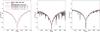 |
Fig. 5 Observed and predicted profiles of hydrogen lines of γ Equ. Dash-dotted lines correspond to He-weak model. |
Figure 5 compares the observed and predicted profiles of hydrogen lines. The normalization of UVES data at the Hβ line was found to suffer considerably from the data processing inaccuracies. Therefore we used observed profile taken with GIRAFFE instrument at SAAO. The normalization of the STIS data in the same region is also not trivial but easier to perform due to its lower resolution and a wide wavelength coverage. On the other hand, Hα line of STIS data is still satisfactorly fitted with Teff = 7550 K models, though the UVES profile lies systematically higher, and thus lower Teff is needed to fit it. The underabundance of He formally resulted in an increase in log (g) from 3.8 to 4.0 so that the He-weak model parameters are A = [7550,4.0,2.06 ± 0.05] .
As follows from the results presented above, the most noticeably affected parameter is log (g), which underwent changes from 4.2 to 3.8−4.0 depending upon the helium abundance used. A value of log (g) = 4.2 was used in Ryabchikova et al. (1997, 2002) to fit atomic lines using atmospheric models with a scaled solar abundances, while in our analysis we used model atmospheres and fluxes computed with realistic abundances of the star. Finally, the use of STIS data allowed us to achieve a more detailed fit to the region of the Balmer jump, whose amplitude is very sensitive to the value of log (g).
The vertical distribution profiles of all 18 chemical elements derived with Teff = 7550 K, log (g) = 3.8, He-norm model are presented in Fig. 6. All but REE elements (i.e. Pr and Nd) are found to accumulate at layers just above the photosphere. For elements Ti and Ba, stratification is not well constrained and probably is not present in the atmosphere of this star at all. A cloud of Pr and Nd is observed at high atmospheres and the abundance gradients of these elements, together with Fe and Si, are the largest among the studied elements.
 |
Fig. 6 Depth-dependent distribution profiles of chemical elements in the atmosphere of γ Equ. |
4.3. 33 Lib (HD 137949)
In the present investigation 33 Lib is the last target analyzed. It is a bright roAp star with many references available regardless its spectroscopic and photometric properties. Unfortunately, no spectroscopic energy distribution is available similar to what is provided by STIS, therefore a fit was done to the ground-based spectrophotometric data from Adelman et al. (1989). Our fitting began with Teff = 7550 K, log (g) = 4.3 model used by Ryabchikova et al. (2004, 2008). Stratification of Si, Fe, Ca, and Cr was derived and accounted for in the model atmosphere calculations. Average abundances of the REE are higher in 33 Lib than in γ Equ by more than an order of magnitude. The stronger magnetic field of ⟨ Bs ⟩ = 5 kG (Ryabchikova et al. 2008), together with high REE abundances, results in extremely strong blending that prevents the proper choice of spectral lines for any stratification study of other elements. It is also the reason we could not perform NLTE stratification analysis of Pr and Nd based on equivalent widths and pseudomicroturbulence approximation of magnetic effects. It could only be done by properly including the magnetic field in NLTE line formation code. Pr-Nd stratification is expected to be rather strong in 33 Lib because of the highest Pr-Nd anomaly observed in this star (Ryabchikova et al. 2004); however, at present step we limit ourselves by taking the average observed REE anomalies into account.
The best-fit parameters are [7400,4.0,2.13 ± 0.13] for both He-norm and He-weak models. As shown in Fig. 7, also [7300,3.8,2.19 ± 0.13] and [7500,4.0,2.06 ± 0.13] models provide a reasonable fit, but with more pronounced deviations between the observed and predicted SEDs at short and long wavelengths.
Similar to other cases described above, for 33 Lib we also found it difficult to fit the Balmer Hα line with the model parameters required to fit the SED (see Fig. 8). A higher Teff is required to fit the observed profile of this line. On the other hand, Hβ and Hγ lines are a satisfactory fit with the Teff = 7400 K model.
The depth-dependent distribution of elements derived using the [7400,4.0] He-norm and He-weak models is shown in Fig. 9. As expected, in both cases the stratification profiles are very similar, with large abundance jumps at deep atmospheric layers.
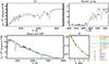 |
Fig. 7 Observed and predicted energy distributions of 33 Lib for two best-fitted models with solar and depleted helium contents. |
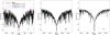 |
Fig. 8 Observed and predicted profiles of hydrogen lines of 33 Lib. |
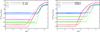 |
Fig. 9 Depth-dependent distribution profiles of chemical elements in the atmosphere of 33 Lib for He-norm and He-weak Teff = 7400 K, log (g) = 4.0 models (left panel), and two He-weak Teff = 7400 K, log (g) = 4.0, and Teff = 7500 K, log (g) = 4.0 models (right panel). |
5. Discussion and conclusions
In an attempt to construct self-consistent models of Ap-star atmospheres, we performed a simultaneous model fit to a number of observed datasets, such as photometric wide-band fluxes, low- and middle-resolution spectrophotometric observations, and high-resolution spectra. Ideally, all of them must be fitted with a single model atmosphere and abundance pattern. The results of the present investigation suggest that this is indeed possible to accomplish by applying a realistic chemical composition and appropriate model atmospheres that account for the peculiar nature of CP stars.
However, a few problems still exist. The most disturbing one is a systematic discrepancy between effective temperatures derived separately from SED and H-lines. In the case of β CrB, only Hα and Hβ agree with SED, but Hγ requires lower Teff. For 33 Lib the situation is the opposite with Hβ and Hγ in agreement with the Teff derived from SED, but Hα clearly requires higher Teff. A good match to SED, Hα, and Hβ was obtained for γ Equ, though no high-resolution data was available for the Hγ line region. Since at least two out of three hydrogen lines always agree with the atmospheric parameters derived from fitting the SED, it is likely that we face the usual problem of continuum normalization of the hydrogen lines in cross-dispersed echelle observations. Thus, one should always be cautious when determining atmospheric parameters solely based on the fit to hydrogen lines.
The abundance and stratification analysis was done using carefully selected spectral lines with accurately known transition parameters, and yet there seems to be a missing absorption in the models of β CrB in UV region blueward λ2500 (see top left panel of Fig. 1). A secondary component is by far too faint and cool to influence the flux in that spectral region.
For β CrB we find a noticeable deviation between the space- and ground-based observations of the SEDs in the visual and NIR regions. A natural reason could be a discrepancy between different flux calibration schemes, which by default are more challenging in the case of ground-based observations. This deviation is seen as a vertical offset in the observed fluxes. It does not affect the determination of Teff (Fig. 1), but does affect the radius estimate by about 0.2 R⊙. This is quite a noticeable uncertainty that highlights once again the need to have accurately calibrated fluxes for stellar parameter determinations.
All previous spectroscopic studies resulted in the log (g) values that were substantially over-estimated, as shown by direct fits presented in Figs. 1, 4, and 7. Our values come mainly from the detailed fit to the amplitude and slope of the Balmer jump based on realistic model atmospheres. Previously, only H-lines, photometric colors and/or low-resolution spectrophotometry by Adelman et al. (1989) were used in combination with scaled-solar metallicity models that did not account for individual abundances, magnetic fields, and improved REE opacity.
We find that possible He depletion of Ap-star atmospheres has minor effect on determining element distributions and log (g), at least for the hottest star considered here, β CrB (see Fig. 3). Formally, an underabundance of He results in choosing a slightly higher log (g) by about 0.1 dex and a cooler Teff by ≈50 K. This change is small and well within the error bars of our fitting procedure. The choice of temperature has a somewhat stronger or at least a comparable impact on the derived stratification profiles of chemical elements, as can be seen from the example of 33 Lib illustrated in left- and right-hand panels of Fig. 9. In particular, a change of ΔTeff = 100 K influences both positions and amplitudes of the abundance jumps. It is important to realize, however, that even if we are not absolutely precise in deriving Teff and know nothing about the real He content of the Ap-star atmospheres, the inferred element stratifications are still informative and stable. Additional uncertainties could result from particular limitations in our fitting procedure (e.g., step-like approximation of stratification profiles, a small number of spectral lines used, etc.), and thus the presented analysis can only provide a general picture of the element distributions in the atmospheres of investigated stars. Still, this is enough to reveal an accumulation of a particular element in the lower or upper atmospheric layers, determine the amplitudes of abundance jumps, and estimate uncertainties in the derived distributions due to assumed model parameters – questions we were mainly interested in.
Interferometry has recently brought an entirely new possibility of measuring the radii of main-sequence stars on a model-independent and regular basis, though its modern instrumental capabilities are limited to bright nearby stars. Our model-based comparison of the observed and predicted SEDs led to good agreement (within error bars) with interferometric estimates as summarized in Table 1. The table also includes calculated masses and luminosities from derived effective temperatures, radii, and gravities. The corresponding error bars were calculated using individual uncertainties of stellar parallaxes along with typical uncertainties of ΔTeff = 50 K and Δlog (g) = 0.1 dex associated with the fit of SEDs and hydrogen line profiles. Large error bars found for HD 103498 are entirely due to a large parallax uncertainty (π = 3.37 ± 0.56 mas given by van Leeuwen 2007).
Figure 10 shows the positions of stars from Table 1 in the H-R diagram along with theoretical evolutionary tracks. This comparison allows deriving stellar masses and ages under a reasonable assumption about the bulk stellar metallicity. Our spectroscopically derived masses generally show good agreement with the theoretical values predicted by evolutionary models within estimated error bars. The only exception is HD 101065 for which evolutionary models predict M = 1.48 M⊙, while Shulyak et al. (2010b) estimates 2.27 ± 0.59 M⊙. In this particular case, however, the derived log (g) was very sensitive to the assumed line opacity of REE elements that were found to affect model fluxes in the Balmer jump region in a dramatic way. Because of NLTE effects and the possible incompleteness of REE line lists, the published value of log (g) = 4.2 derived from the fit to the observed SED could easily be overestimated, and a somewhat lower log (g) = 4.0 would give a consistent mass estimate.
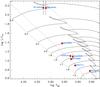 |
Fig. 10 Predicted location of Ap stars in the H-R diagram for the luminosity and temperature estimates from Table 1. Theoretical evolutionary tracks were adopted from Girardi et al. (2000) for the bulk metallically of Z = 0.018. The dotted lines show ZAMS, 50% fractional main sequence age line, and TAMS. |
Acknowledgments
We thank Dr. Igor Savanov for kindly providing us with Hβ spectrum of β CrB. This work was supported by the following grants: Deutsche Forschungsgemeinschaft (DFG) Research Grant RE1664/7-1 to D.S. and Basic Research Program of the Russian Academy of Sciences “Nonstationary phenomena in the Universe” to T.R. OK is a Royal Swedish Academy of Sciences Research Fellow supported by grants from the Knut and Alice Wallenberg Foundation and from the Swedish Research Council. Some of the data presented in this paper were obtained from the Mikulski Archive for Space Telescopes (MAST). STScI is operated by the Association of Universities for Research in Astronomy, Inc., under NASA contract NAS5-26555. Support for MAST for non-HST data is provided by the NASA Office of Space Science via grant NNX09AF08G and by other grants and contracts. We also acknowledge the use of electronic databases (VALD, SIMBAD, NASA’s ADS) and cluster facilities at the Vienna Institute for Astronomy and Georg August University Göttingen.
References
- Adelman, S. J., Pyper, D. M., Shore, S. N., White, R. E., & Warren, W. H., Jr. 1989, A&AS, 81, 221 [NASA ADS] [Google Scholar]
- Alekseeva, G. A., Arkharov, A. A., Galkin, V. D., et al. 1996, Baltic Astron., 5, 603 [Google Scholar]
- Armstrong, N. M. R., Rosner, S. D., & Holt, R. A. 2011, Phys. Scr., 84, 055301 [NASA ADS] [CrossRef] [Google Scholar]
- Bergemann, M., Pickering, J. C., & Gehren, T. 2010, MNRAS, 401, 1334 [NASA ADS] [CrossRef] [Google Scholar]
- Blackwell-Whitehead, R. J., Pickering, J. C., Pearse, O., & Nave, J. 2003, ApJS, 157, 402 [Google Scholar]
- Boiarchuk, A. A. 1986, Itogi Nauki i Tekhniki Seriia Astronomiia, 31, 198 [NASA ADS] [Google Scholar]
- Boksenberg, A., Evans, R. G., Fowler, R. G., et al. 1973, MNRAS, 163, 291 [NASA ADS] [Google Scholar]
- Breger, M. 1976, ApJS, 32, 7 [NASA ADS] [CrossRef] [Google Scholar]
- Bruntt, H., North, J. R., Cunha, M., et al. 2008, MNRAS, 386, 2039 [NASA ADS] [CrossRef] [Google Scholar]
- Bruntt, H., Kervella, P., Mérand, A., et al. 2010, A&A, 512, A55 [NASA ADS] [CrossRef] [EDP Sciences] [Google Scholar]
- Cowley, C. R., Hubrig, S., Castelli, F., González, J. F., & Wolff, B. 2007, MNRAS, 377, 1579 [NASA ADS] [CrossRef] [Google Scholar]
- Dekker, H., D’Odorico, S., Kaufer, A., Delabre, B., & Kotzlowski, H. 2000, Proc. SPIE, 4008, 534 [Google Scholar]
- Fabricius, C., Høg, E., Makarov, V. V., et al. 2002, A&A, 384, 180 [NASA ADS] [CrossRef] [EDP Sciences] [Google Scholar]
- Ginibre, A. 1989, Phys. Scr., 39, 710 [NASA ADS] [CrossRef] [Google Scholar]
- Girardi, L., Bressan, A., Bertelli, G., & Chiosi, C. 2000, A&AS, 141, 371 [NASA ADS] [CrossRef] [EDP Sciences] [Google Scholar]
- Holt, R. A., Scholl, T. J., & Rosner, S. D. 1999, MNRAS, 306, 107 [NASA ADS] [CrossRef] [Google Scholar]
- Khan, S. A., & Shulyak, D. V. 2006a, A&A, 448, 1153 [NASA ADS] [CrossRef] [EDP Sciences] [Google Scholar]
- Khan, S. A., & Shulyak, D. V. 2006b, A&A, 454, 933 [NASA ADS] [CrossRef] [EDP Sciences] [Google Scholar]
- Kochukhov, O. 2007, in Physics of Magnetic Stars, eds. D. O. Kudryavtsev, & I. I. Romanyuk, Nizhnij Arkhyz., 109 [Google Scholar]
- Kochukhov, O., Shulyak, D., & Ryabchikova, T. 2009, A&A, 499, 85 [Google Scholar]
- Komarov, N. S., Dragunova, A. V., Belik, S. I., et al. 1995, Odessa Astron. Publ., 8, 3 [NASA ADS] [Google Scholar]
- Krtička, J., Mikulášek, Z., Lüftinger, T., et al. 2012, A&A, 537, A14 [NASA ADS] [CrossRef] [EDP Sciences] [Google Scholar]
- Kupka, F., Piskunov, N., Ryabchikova, T. A., Stempels, H. C., & Weiss, W. W. 1999, A&AS, 138, 119 [NASA ADS] [CrossRef] [EDP Sciences] [MathSciNet] [PubMed] [Google Scholar]
- Kurtz, D. W., Elkin, V. G., & Mathys, G., 2006, MNRAS, 370, 1274 [NASA ADS] [CrossRef] [Google Scholar]
- Kurucz, R. L. 1992, The Stellar Populations of Galaxies, 149, 225 [NASA ADS] [CrossRef] [Google Scholar]
- Kurucz, R. 1993, ATLAS9 Stellar Atmosphere Programs and 2 km s-1 grid. Kurucz CD-ROM 13 (Cambridge, Mass.: Smithsonian Astrophysical Observatory), 1993, 13 [Google Scholar]
- Leblanc, F., & Monin, D. 2004, The A-Star Puzzle, 224, 193 [Google Scholar]
- Mashonkina, L., Ryabchikova, T., & Ryabtsev, A. 2005, A&A, 441, 309 [NASA ADS] [CrossRef] [EDP Sciences] [Google Scholar]
- Mashonkina, L., Ryabchikova, T., Ryabtsev, A., & Kildiyarova, R. 2009, A&A, 495, 297 [NASA ADS] [CrossRef] [EDP Sciences] [Google Scholar]
- Michaud, G., Martel, A., Montmerle, T., et al. 1979, ApJ, 234, 206 [NASA ADS] [CrossRef] [Google Scholar]
- North, P., Carquillat, J.-M., Ginestet, N., Carrier, F., & Udry, S. 1998, A&AS, 130, 223 [NASA ADS] [CrossRef] [EDP Sciences] [Google Scholar]
- Pandey, C. P., Shulyak, D. V., Ryabchikova, T., & Kochukhov, O. 2011, MNRAS, 417, 444 [NASA ADS] [CrossRef] [Google Scholar]
- Perraut, K., Brandão, I., Mourard, D., et al. 2011, A&A, 526, A89 [NASA ADS] [CrossRef] [EDP Sciences] [Google Scholar]
- Pickering, J. C. 2006, ApJS, 107, 811 [Google Scholar]
- Piskunov, N. E., Kupka, F., Ryabchikova, T. A., Weiss, W. W., & Jeffery, C. S. 1995, A&AS, 112, 525 [NASA ADS] [Google Scholar]
- Ryabchikova, T. A., Adelman, S. J., Weiss, W. W., & Kuschnig, R. 1997, A&A, 322, 234 [NASA ADS] [Google Scholar]
- Ryabchikova, T., Piskunov, N., Kochukhov, O., et al. 2002, A&A, 384, 545 [NASA ADS] [CrossRef] [EDP Sciences] [Google Scholar]
- Ryabchikova, T., Nesvacil, N., Weiss, W. W., Kochukhov, O., & Stütz, C. 2004, A&A, 423, 705 [NASA ADS] [CrossRef] [EDP Sciences] [Google Scholar]
- Ryabchikova, T., Leone, F., & Kochukhov, O. 2005, A&A, 438, 973 [NASA ADS] [CrossRef] [EDP Sciences] [Google Scholar]
- Ryabchikova, T., Sachkov, M., Kochukhov, O., Lyashko, D. 2007, A&A, 473, 907 [NASA ADS] [CrossRef] [EDP Sciences] [Google Scholar]
- Ryabchikova, T., Kochukhov, O., & Bagnulo, S. 2008, A&A, 480, 811 [NASA ADS] [CrossRef] [EDP Sciences] [Google Scholar]
- Savanov, I. S., & Kochukhov, O. P. 1998, Astron. Lett., 24, 516 [NASA ADS] [Google Scholar]
- Shulyak, D., Tsymbal, V., Ryabchikova, T., Stütz, Ch., & Weiss, W. W. 2004, A&A, 428, 993 [NASA ADS] [CrossRef] [EDP Sciences] [Google Scholar]
- Shulyak, D., Ryabchikova, T., Mashonkina, L., & Kochukhov, O. 2009, A&A, 499, 879 [NASA ADS] [CrossRef] [EDP Sciences] [Google Scholar]
- Shulyak, D., Krtička, J., Mikulášek, Z., Kochukhov, O., & Lüftinger, T. 2010a, A&A, 524, A66 [NASA ADS] [CrossRef] [EDP Sciences] [Google Scholar]
- Shulyak, D., Ryabchikova, T., Kildiyarova, R., & Kochukhov, O. 2010b, A&A, 520, A88 [NASA ADS] [CrossRef] [EDP Sciences] [Google Scholar]
- Thompson, G. I., Nandy, K., Jamar, C., et al. 1978, The Science Research Council, UK [Google Scholar]
- Tokovinin, A. A. 1984, Pis’ma Astronomicheskii Zhurnal, 10, 293 [NASA ADS] [Google Scholar]
- Tsymbal, V., Lyashko, D., & Weiss, W. W. 2003, Mod. Stellar Atmosph., 210, 49 [Google Scholar]
- van Leeuwen, F. 2007, A&A, 474, 653 [NASA ADS] [CrossRef] [EDP Sciences] [Google Scholar]
- Villemoes, P., Arnesen, A. F., Heijkenskjóld, A, et al. 1992, Phys. Scr., 46, 45 [NASA ADS] [CrossRef] [Google Scholar]
All Tables
All Figures
|
Fig. 1 Observed and predicted energy distributions of β CrB for two best-fitted models with solar and depleted helium contents. |
| In the text | |
|
Fig. 2 Observed and predicted profiles of hydrogen lines of β CrB. Full line – He norm model; dashed line – He-weak model. |
| In the text | |
|
Fig. 3 Depth-dependent distribution profiles of chemical elements in the atmosphere of β CrB. |
| In the text | |
|
Fig. 4 Observed and predicted energy distributions of γ Equ for two best-fitted models with solar and depleted helium contents. |
| In the text | |
|
Fig. 5 Observed and predicted profiles of hydrogen lines of γ Equ. Dash-dotted lines correspond to He-weak model. |
| In the text | |
|
Fig. 6 Depth-dependent distribution profiles of chemical elements in the atmosphere of γ Equ. |
| In the text | |
|
Fig. 7 Observed and predicted energy distributions of 33 Lib for two best-fitted models with solar and depleted helium contents. |
| In the text | |
|
Fig. 8 Observed and predicted profiles of hydrogen lines of 33 Lib. |
| In the text | |
|
Fig. 9 Depth-dependent distribution profiles of chemical elements in the atmosphere of 33 Lib for He-norm and He-weak Teff = 7400 K, log (g) = 4.0 models (left panel), and two He-weak Teff = 7400 K, log (g) = 4.0, and Teff = 7500 K, log (g) = 4.0 models (right panel). |
| In the text | |
|
Fig. 10 Predicted location of Ap stars in the H-R diagram for the luminosity and temperature estimates from Table 1. Theoretical evolutionary tracks were adopted from Girardi et al. (2000) for the bulk metallically of Z = 0.018. The dotted lines show ZAMS, 50% fractional main sequence age line, and TAMS. |
| In the text | |
Current usage metrics show cumulative count of Article Views (full-text article views including HTML views, PDF and ePub downloads, according to the available data) and Abstracts Views on Vision4Press platform.
Data correspond to usage on the plateform after 2015. The current usage metrics is available 48-96 hours after online publication and is updated daily on week days.
Initial download of the metrics may take a while.