| Issue |
A&A
Volume 551, March 2013
|
|
|---|---|---|
| Article Number | A140 | |
| Number of page(s) | 5 | |
| Section | Atomic, molecular, and nuclear data | |
| DOI | https://doi.org/10.1051/0004-6361/201219491 | |
| Published online | 11 March 2013 | |
On the X 1Σ+ rovibrational spectrum of lithium hydride
1 Department of Physics and Astronomy and the Center for Simulational PhysicsUniversity of Georgia, Athens, GA 30602, USA
e-mail: This email address is being protected from spambots. You need JavaScript enabled to view it.
2 Institute of Applied Physics and Computational Mathematics, 100094 Beijing, PR China
e-mail: This email address is being protected from spambots. You need JavaScript enabled to view it.
; This email address is being protected from spambots. You need JavaScript enabled to view it.
Received: 26 April 2012
Accepted: 21 January 2013
Abstract
The complete line list of rovibrational transitions of the X 1Σ+ state of LiH is computed. The line list includes all possible dipole-allowed transition energies and oscillator strengths that cover the transition energy range 3.27 − 19476 cm-1. The line list was obtained using an accurate potential and dipole moment function constructed from available experimental and theoretical data. This paper discusses the agreement of the current calculations with previous theoretical and experimental results. We also provide the radiative cooling function in the high-density limit over a wide temperature range and compare them with previous results. A simulated collisionally-broadened LiH opacity relevant to cool dwarf stars is also presented.
Key words: molecular data / molecular processes
© ESO, 2013
1. Introduction
Lithium hydride has been the subject of theoretical and experimental molecular physics investigations for many years (see for example Partridge & Langhoff 1981). As the simplest neutral heteronuclear diatomic molecule, LiH is a favorite benchmark for various quantum-chemical techniques (Tung et al. 2011; Holka et al. 2011). In astrophysics, LiH may play a role at temperatures T ≤ 5000 K in the cooling of primordial clouds (Stancil et al. 1996; Bougleux & Galli 1997; Galli & Palla 1998; Bovino et al. 2011) and is a means of monitoring the evolution of stars and interstellar clouds (Dulick et al. 1998). Furthermore, LiH, as well as other Li-bearing molecules (LiCl and LiOH), may be observable in cool (Teff ≤ 2000 K) dwarf atmospheres (Lodders 1999; Weck et al. 2004). However, to date, searches for LiH at high redshift have proved unsuccessful (Friedel et al. 2011). Reviews of the lithium chemistry in the early Universe have been given by Lepp et al. (2002) and Bovino et al. (2011), while the status of laboratory infrared spectroscopy of LiH is outlined in Dulick et al. (1998). A complete and evaluated rovibrational line list for the ground electronic state, which is germane to its thermal evolution and needed for primordial spectral models, is needed1.
In Sect. 2 we present the details of potential energy curve and dipole moment function for the electronic ground state of LiH. In Sect. 3, we briefly outline the relevant relations for computing transition energies, Einstein coefficients, oscillator strengths, and radiative cooling functions. Results of the current computation including the ground electronic-state rovibrational line list and cooling function are presented in Sect. 4 along with comparisons to previous work and astrophysical applications. Section 5 gives a summary of the current work. Atomic units are used throughout, unless otherwise noted.
2. Potential energy and dipole moment function
Within the well-known Born-Oppenheimer approximation, the motion of a diatomic molecule may be partitioned into its electronic and nuclear components. As such, the non-relativistic Hamiltonian of a molecule may be written as  (1)with the time-independent Schrödinger equation given by
  (2)By separation of variables, the total wave function may be written as
 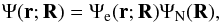 (3)where R is the internuclear distance vector in body-fixed coordinates, and r the electron coordinate vector with respect to the center of mass of the nuclei. The motion of electrons (e) and nuclei (N) can be described by the electronic Schrödinger equation
  (4)and the nuclear Schrödinger equation
 ![Mathematical equation: \begin{equation} [\hat{T}_{\rm N}+E_{\rm e}(\vec{R})]\Psi_{\rm N}(\vec{R})=E_{\nu J}\Psi_{\rm N}(\vec{R}), \end{equation}](/articles/aa/full_html/2013/03/aa19491-12/aa19491-12-eq13.png) (5)where Ee(R) is the potential energy and Ev,J the rovibrational energy or eigenvalue.
(5)where Ee(R) is the potential energy and Ev,J the rovibrational energy or eigenvalue.
The dipole moment function can be defined as  (6)where Ψe(r;R) is the electronic eigenfunction. In this work we consider X1Σ+ ← X1Σ+ rovibrational transitions so that only the z-component of the r operator contributes.
For a diatomic molecule, the potential energy is only a function of nuclear distance and can be written as Ee(R). We applied an empirical potential (Coxon & Dickinson 2004), which was generated by directly fitting the spectroscopic LiH line positions, for 2 < R < 20 a0. The long-range potential is given by  for R > 20 a0, where C6 = 66.536, C8 = 3279.99 and C10 = 223016.6 (Yan et al. 1996). For R < 2 a0, the potential has been extrapolated with the short-range form VSR(R) = Aexp( − BR) + C.
In a similar way, the dipole moment function of the X state calculated by Partridge & Langhoff (1981) has been used over the range R = 1.75 to 17.5 a0. For R > 17.5 a0, the long-range form of Bottcher & Dalgarno (1974), DLR(R) = d7/R7, was adopted. For R < 1.75 a0, the short-range form DSR(R) = AR2 + BR was fit to the ab initio data. The potential and dipole moment function are displayed in Fig. 1.
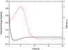 |
Fig. 1 Potential energy (solid line) and the dipole moment function (dashed line) of the X |
3. Rovibrational eigenvalues, transition probabilities, and related quantities
The radial nuclear Schrödinger equation of a diatomic molecule may be written as ![Mathematical equation: \begin{equation} \left[ -\frac{1}{2 \mu}\frac{{\rm d}^2}{{\rm d}R^2}+E_{\rm e}(R)+\frac{J(J+1)}{2 \mu R^2}-E_{vJ}\right]\chi_{vJ}(R)=0, \label{radSE} \end{equation}](/articles/aa/full_html/2013/03/aa19491-12/aa19491-12-eq37.png) (7)which can be solved numerically by the Numerov-Cooley method (Johnson 1977), for example. Here μ is the reduced mass of 7LiH, ν is vibrational quantum number, J the rotational quantum number, and χvJ(R) is the corresponding rovibrational eigenfunction. The Einstein A coefficient, or transition probability, in the dipole approximation, can be calculated given χvJ(R) and D(R), and is defined as (Weissbluth 1978)
(7)which can be solved numerically by the Numerov-Cooley method (Johnson 1977), for example. Here μ is the reduced mass of 7LiH, ν is vibrational quantum number, J the rotational quantum number, and χvJ(R) is the corresponding rovibrational eigenfunction. The Einstein A coefficient, or transition probability, in the dipole approximation, can be calculated given χvJ(R) and D(R), and is defined as (Weissbluth 1978) 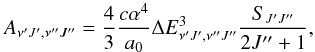 (8)where α = e2/ħc, is the fine-structure constant, a0 is the Bohr radius, and ΔEν′J′,ν′′J′′ the transition energy. Here SJ′J′′ is the line strength and defined as
  (9)Here ϕJ′J′′ is a Hönl-London factor (Herzberg 1989) given by
 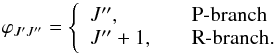 (10)The oscillator strength may then be defined (Weissbluth 1978) as
  (11)In a variety of applications, it is useful to obtain the radiative cooling function in the high-density or local thermodynamic equilibrium (LTE) limit (see for example Coppola et al. 2011). In LTE, the radiative cooling function only depends on the rovibrational energies, degeneracies, and transition probabilities. It is only a function of the gas kinetic temperature T and is given (in ergs/s) by
 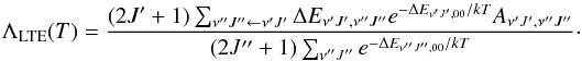 (12)The sum is over all possible rovibrational deexcitation transitions within the electronic ground state and the denominator is the rovibrational partition function Q(T).
4. Results and discussion
The radial Schrödinger Eq. (7) was solved with a step size 1.0 × 10⁻³a0, over a range of internuclear distances from R = 1.0 to 60.0 a0. The reduced mass of 7LiH was 0.881238162 u (Stwalley & Zemke 1993).
Vibrational binding energies Gν′ of the X1Σ+ state of 7LiH in units of cm-1.
The vibrational energies Gν′ and corresponding vibrational energy spacings ΔGν′ + 1/2 of the X 1Σ+ state obtained in the present study are listed in Tables 1 and 2, along with the theoretical values of Holka et al. (2011) and the measurements of Chan et al. (1986). The largest discrepancy for Gν′ between our calculations and the experiment is 2.47 cm-1, which occurs for v = 22, while the largest difference for ΔGν′ + 1/2 is smaller at 1.85 cm-1 for v = 22. Some select transition energies are listed in Table 3 along with the corresponding experimental results of Dulick et al. (1998) and the calculations of Coppola et al. (2011). It can be seen that the current results are in excellent agreement with experiments, the largest discrepancy being 0.027 cm-1.
Transition probabilities for some band-averaged transitions in the X1Σ+ state are compared in Table 4 with the previous calculation of Partridge & Langhoff (1981). The maximum difference is less than 6.79%. As a further illustration, the J-dependent dipole moment matrix elements for v = 1 to v = 0 are shown in Fig. 2. which are similar to those given in Gianturco et al. (1996). It can be seen that the transition probabilities for the P-branch are much higher than those for the R-branch. The line oscillator strengths as a function of wavelength are shown in Fig. 3 for the X  X
X  transition. The most intense line of the R-branch is at 22.968 μm (band 0-0, R(60)). For the P-branch, the strongest is at 16.822 μm (band 8-7, P(31)). The complete line list is available on the UGA Molecular Opacity Project website (http://www.physast.uga.edu/ugamop/) and in the format of the Leiden Atomic and Molecular Database (LAMDA, Schöier et al. 2005).
Utilizing the theoretical rovibrational energies and transition probabilities, the LTE radiative cooling function was calculated as a function of temperature as shown in Fig. 4. It is compared with the previous results of Dalgarno (1994, priv. comm.) and Coppola et al. (2011), along with the low-density limit cooling function (nH ≤ 100 cm-3) due to H collisions (Galli & Palla 1998) (see the Appendix for a further discussion). All three LTE cooling functions are seen to be in excellent agreement over the considered temperature range.
Vibrational level spacings ΔGν′ + 1/2 of the X state of 7LiH where ΔGν′ + 1/2 = Gν′ + 1 − Gν′ is in units of cm-1.
Rovibrational transition energies for in the X 1Σ+ state of 7LiH.
A-values for transitions in the X 1Σ+ state of 7LiH.
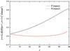 |
Fig. 2 Dipole moment matrix elements for the P-branch and R-branch rovibrational transitions for 7LiH for the v = 0 to v = 1 transition. |
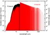 |
Fig. 3 Oscillator strengths for the X |
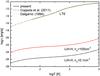 |
Fig. 4 Radiative cooling functions of LiH in the LTE (upper three lines) and the low-density limit (nH ≤ 100 cm-3, lower solid red and black lines) considering only H collisions. |
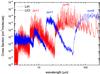 |
Fig. 5 Opacity of the LiH (red) rovibrational transitions in the infrared compared to the LiCl (blue) opacity for a temperature of 1800 K and a pressure of 100 atms. |
To simulate the opacity of LiH in a cool dwarf atmosphere, we computed the absorption cross section using Eq. (6) of Dulick et al. (2003) for a temperature of 1800 K, as an example. The line absorption cross section, which is a function of the transition probability, line frequency, partition function, and temperature, is multiplied by a Lorentzian line profile (Bernath 1995) with width corresponding to collisional broadening. Assuming a canonical collisional broadening cross section of 10-16 cm2 with a line width proportional to the pressure, Figure 5 displays the opacity for 100 atms. There is a series of strong individual pure rotational lines for λ > 20 μm, while the fundamental vibrational band occurs near 8 μm. Comparison is made to the LiCl opacity (Weck et al. 2004) for the same temperature and pressure. The LiCl fundamental vibrational band falls in the gap between the pure LiH rotational lines and the LiH 0-1 band, but is typically one to two orders of magnitude smaller. According to the cool dwarf atmosphere models of Lodders (1999), the abundances of LiH and LiCl, as well as LiOH, are comparable at 1800 K, but for higher temperatures, LiH becomes the dominant Li-bearing molecule. Weck et al. (2004) suggest that it would be difficult to detect LiCl in cool dwarfs due to strong absorption features from other more abundant molecules (e.g., water) in the same wavelength range. LiH, with its somewhat higher opacity,might be a better candidate for detecting lithium molecules.
5. Conclusions
The rovibrational energy levels of 7LiH were computed with an empirical potential generated from a direct fit of available spectroscopic line positions. The computed vibrational energies and transition energies are found to be in very good agreement with experiments. Oscillator strengths and transition probabilities were also computed and used to construct a complete rovibrational line list. The transition energies were evaluated against available experimental data and found to be reliable to better than 0.03 cm-1. The line list was used to compute an LTE radiative cooling function for LiH and to explore its infrared opacity. Among all dominant Li-bearing molecules, LiH is a better candidate for detecting lithium in cool dwarf atmospheres.
Appendix: Collisional excitation of LiH
While in this work, we present an LTE radiative cooling function (i.e., valid within the high-density limit), Bougleux & Galli (1997) have approximated a density-dependent non-LTE (NLTE) cooling function (see also Galli & Palla 1998). In this approach, the NLTE cooling function is parameterized in terms of the LTE radiative cooling function and a collisional cooling function in the zero-density limit. For applications to the early Universe, they considered only collisions due to atomic hydrogen. Unfortunately, rotational or vibrational excitation rate coefficients of LiH due to H are not available, requiring Bougleux & Galli (1997) to adopt the LiH-He calculations of Jendrek & Alexander (1980), but adjusted to emulate LiH-H collisions via mass-scaling of the collisional rate coefficients. The mass-scaling approach is typically adopted when rate coefficients due to He impact are used to approximate para-H2 impact. Recent work on other molecules suggests this approach is questionable at best (e.g., Cernicharo et al. 2011) even though the PESs for He- and H2-complexes are expected to be similar, being characterized by weakly bound van der Waals minima. Collision complexes involving H, on the other hand, typically involve very deep wells leading to very fast exothermic reactive channels. As a consequence, mass-scaling to deduce H-impact excitation rate coefficients from He- or H2-impact data is likely to be a poor approximation.
For general astrophysical applications, collisions due to the most abundant species, H, H2, He, e−, and H+, should be included in an NLTE cooling function, though H2 dominates in most interstellar environments. LiH-He collisional excitation calculations have been more recently given by Taylor & Hinde (1999, 2005) and Bodo et al. (2001a), and discussed in a review of lithium chemistry by Bodo et al. (2003). The reactive process  (13)and the H-exchange process
  (14)have been considered in a number of recent studies (Prudente et al. 2009; Bovino et al. 2009), but to date, inelastic collisional excitation of LiH due to H has not been investigated because it is a very computationally demanding problem that would require simultaneous treatment with reactions (13) and (14). We are unaware of any inelastic data due to H2, e−, or H+ impacts, though an excited state PES for the LiH
 complex is available (Bodo et al. 2001b), which could be used later. It is therefore, not currently possible to construct an accurate, comprehensive NLTE cooling function for LiH. Figure 4 gives an indication of the expected range of the NLTE cooling function.
A previous, though unevaluated, line list is available on the ExoMol database: http://www.exomol.com
Acknowledgments
The work of P.C.S. was partially supported by NSF grant AST-0607733 and NASA grant NNX07AP12G. Y.B.S. acknowledges travel support by the International Cooperation and Exchange Foundation of CAEP. We thank the referee for helpful comments that improved the manuscript.
References
- Bernath, P. F. 1995, Spectra of atoms and molecules (Oxford University Press) [Google Scholar]
- Bodo, E., Gianturco, F. A., & Martinazzo, R. 2001a, Chem. Phys., 271, 309 [NASA ADS] [CrossRef] [Google Scholar]
- Bodo, E., Gianturco, F. A., & Martinazzo, R. 2001b, J. Phys. Chem. A, 105, 10986 [CrossRef] [Google Scholar]
- Bodo, E., Gianturco, F. A., & Martinazzo, R. 2003, Phys. Rep., 384, 85 [NASA ADS] [CrossRef] [Google Scholar]
- Bottcher, C., & Dalgarno, A. 1974, Proc. Roy. Soc. London, Ser. A, 340, 187 [CrossRef] [Google Scholar]
- Bougleux, E., & Galli, D. 1997, MNRAS, 288, 638 [NASA ADS] [Google Scholar]
- Bovino, S., Wernli, M., & Gianturco, F. A. 2009, ApJ, 699, 383 [NASA ADS] [CrossRef] [Google Scholar]
- Bovino, S., Tacconi, M., Gianturco, F. A., Galli, D., & Palla, F. 2011, ApJ, 731, 107 [NASA ADS] [CrossRef] [Google Scholar]
- Cernicharo, J., Spielfiedel, A., Balança, C., et al. 2011, A&A, 531, A103 [NASA ADS] [CrossRef] [EDP Sciences] [Google Scholar]
- Chan, Y. C., Harding, D. R., & Stwalley, W. C. 1986, J. Chem. Phys., 85, 2436 [NASA ADS] [CrossRef] [Google Scholar]
- Coppola, C. M., Lodi, L., & Tennyson, J. 2011, MNRAS, 415, 487 [NASA ADS] [CrossRef] [Google Scholar]
- Coxon, J. A., & Dickinson, C. S. 2004, J. Chem. Phys., 121, 9378 [NASA ADS] [CrossRef] [Google Scholar]
- Dalgarno, A. 1994, unpublished [Google Scholar]
- Dulick, M., Zhang, K. Q., Guo, B., & Bernath, P. F. 1998, J. Mol. Spectrosc., 188, 14 [NASA ADS] [CrossRef] [Google Scholar]
- Dulick, M., Bauschlicher, C. W. Jr., Burrows, A., et al. 2003, ApJ, 594, 651 [NASA ADS] [CrossRef] [Google Scholar]
- Friedel, D. N., Kemball, A., & Fields, B. D. 2011, ApJ, 738, 37 [NASA ADS] [CrossRef] [Google Scholar]
- Galli, D., & Palla, F. 1998, A&A, 335, 403 [NASA ADS] [Google Scholar]
- Gianturco, F. A., Giorgi, P. G., Berriche, H., & Gadea, F. X. 1996, A&AS, 117, 377 [Google Scholar]
- Herzberg, G. 1989, Molecular Structure I, Spectra of Diatomic Molecules, 2nd edn. (Krieger Pub Co.) [Google Scholar]
- Holka, F., Szalay, P. G., Fremont, J., et al. 2011, J. Chem. Phys., 134, 094306 [NASA ADS] [CrossRef] [Google Scholar]
- Jendrek, E. F., & Alexander, M. H. 1980, J. Chem. Phys., 72, 6452 [NASA ADS] [CrossRef] [Google Scholar]
- Johnson, B. R. 1977, J. Chem. Phys., 67, 4086 [NASA ADS] [CrossRef] [Google Scholar]
- Lepp, S., Stancil, P. C., & Dalgarno, A. 2002, J. Phys. B: At. Mol. Opt. Phys., 35, R57 [NASA ADS] [CrossRef] [Google Scholar]
- Lodders, K. 1999, ApJ, 519, 793 [NASA ADS] [CrossRef] [Google Scholar]
- Partridge, H., & Langhoff, S. R. 1981, J. Chem. Phys., 74, 2361 [NASA ADS] [CrossRef] [Google Scholar]
- Prudente, F. V., Marques, J. M. C., & Maniero, A. M. 2009, Chem. Phys. Lett., 474, 18 [NASA ADS] [CrossRef] [Google Scholar]
- Schöier, F. L., van der Tak, F. F. S., van Dishoeck, E. F., & Black, J. H. 2005, A&A, 432, 369 [NASA ADS] [CrossRef] [EDP Sciences] [Google Scholar]
- Stancil, P. C., Lepp, S., & Dalgarno, A. 1996, ApJ, 458, 401 [NASA ADS] [CrossRef] [Google Scholar]
- Stwalley, W. C., & Zemke, W. T. 1993, J. Phys. Chem. Ref. Data, 22, 87 [NASA ADS] [CrossRef] [Google Scholar]
- Taylor, B. K., & Hinde, R. J. 1999, J. Chem. Phys., 111, 973 [NASA ADS] [CrossRef] [Google Scholar]
- Taylor, B. K., & Hinde, R. J. 2005, J. Chem. Phys., 122, 074308 [NASA ADS] [CrossRef] [Google Scholar]
- Tung, W.-C., Pavanello, M., & Adamowicz, L. 2011, J. Chem. Phys., 134, 064117 [NASA ADS] [CrossRef] [Google Scholar]
- Weck, P. F., Schweitzer, A., Kirby, K., Haushildt, P. H., & Stancil, P. C. 2004, ApJ, 613, 567 [NASA ADS] [CrossRef] [Google Scholar]
- Weissbluth, M. 1978, Atoms and Molecules (Academic press) [Google Scholar]
- Yan, Z. C., Babb, J. F., Dalgarno, A., & Drake, G. W. F. 1996, Phys. Rev. A, 54, 2824 [NASA ADS] [CrossRef] [PubMed] [Google Scholar]
All Tables
Vibrational level spacings ΔGν′ + 1/2 of the X state of 7LiH where ΔGν′ + 1/2 = Gν′ + 1 − Gν′ is in units of cm-1.
All Figures
|
Fig. 1 Potential energy (solid line) and the dipole moment function (dashed line) of the X |
| In the text | |
|
Fig. 2 Dipole moment matrix elements for the P-branch and R-branch rovibrational transitions for 7LiH for the v = 0 to v = 1 transition. |
| In the text | |
|
Fig. 3 Oscillator strengths for the X |
| In the text | |
|
Fig. 4 Radiative cooling functions of LiH in the LTE (upper three lines) and the low-density limit (nH ≤ 100 cm-3, lower solid red and black lines) considering only H collisions. |
| In the text | |
|
Fig. 5 Opacity of the LiH (red) rovibrational transitions in the infrared compared to the LiCl (blue) opacity for a temperature of 1800 K and a pressure of 100 atms. |
| In the text | |
Current usage metrics show cumulative count of Article Views (full-text article views including HTML views, PDF and ePub downloads, according to the available data) and Abstracts Views on Vision4Press platform.
Data correspond to usage on the plateform after 2015. The current usage metrics is available 48-96 hours after online publication and is updated daily on week days.
Initial download of the metrics may take a while.