© ESO, 2013

1. Introduction

A growing body of evidence indicates that interstellar filaments play a fundamental role in the star formation process. In particular, the results from the Herschel Gould Belt survey (HGBS) confirm the omnipresence of parsec-scale filaments in nearby molecular clouds and suggest that the observed filamentary structure is directly related to the formation of prestellar cores (André et al. 2010). While molecular clouds such as Taurus were already known to exhibit large-scale filamentary structures long before Herschel (cf. Schneider & Elmegreen 1979; Goldsmith et al. 2008), the Herschel observations now demonstrate that filaments are truly ubiquitous in the cold interstellar medium (ISM) (see Men’shchikov et al. 2010; Molinari et al. 2010; Arzoumanian et al. 2011). Furthermore, the Herschel results indicate that the inner width of the filaments is quasi-universal at ~0.1 pc (Arzoumanian et al. 2011).

The characteristic filament width corresponds to within a factor of ~2 to the sonic scale around which the transition between supersonic and subsonic turbulent motions occurs in diffuse, non-star-forming gas and a change in the slope of the linewidth-size relation is observed (cf. Goodman et al. 1998; Falgarone et al. 2009; Federrath et al. 2010). This similarity suggests that the formation of filaments may result from turbulent compression of interstellar gas in low-velocity shocks (cf. Padoan et al. 2001). Alternatively, the characteristic width may also be understood if interstellar filaments are formed as quasi-equilibrium structures in pressure balance with a typical ambient ISM pressure P_ext ~ 2−5 × 10⁴ K cm^-3 (Fischera & Martin 2012, Inutsuka et al. in prep.).

The HGBS observations also show that the prestellar cores identified with Herschel in active star-forming regions such as the Aquila Rift cloud (cf. Könyves et al. 2010) are primarily located within the densest filaments for which the mass per unit length exceeds the critical value (e.g., Inutsuka & Miyama 1997), ${\mathit{M}}_{\mathrm{line}\mathit{,}\mathrm{crit}}\mathrm{=}\mathrm{2}{\mathit{c}}_{\mathrm{s}}^{\mathrm{2}}\mathit{/}\mathit{G}\mathrm{~}\mathrm{15}{\mathit{M}}_{\mathrm{\odot }}$/pc, where c_s ~ 0.2 km s^-1 is the isothermal sound speed for T ~ 10 K. These Herschel results support a scenario according to which core formation occurs in two main steps (e.g., André et al. 2010, 2011). First, large-scale magneto-hydrodynamic (MHD) turbulence gives rise to a web-like network of filaments in the ISM. In a second step, gravity takes over and fragments the densest filaments into prestellar cores via gravitational instability. Indirect arguments suggest that dense, self-gravitating filaments, which are expected to undergo radial contraction (e.g. Inutsuka & Miyama 1997), can maintain a constant central width of 0.1 pc if they accrete additional mass from their surroundings while contracting (Arzoumanian et al. 2011).

We present new Herschel observations taken as part of the HGBS toward and around the B211/B213 filament in the Taurus molecular cloud. We suggest that this filament is indeed gaining mass from a neighboring network of lower-density striations elongated parallel to the magnetic field (see also Goldsmith et al. 2008). Owing to its close distance to the Sun (d ~ 140 pc – Elias 1978), the Taurus cloud has been the subject of numerous observational and theoretical studies. In particular, it has long been considered as a prototypical region and has inspired magnetically-regulated models of low-mass, dispersed star formation (e.g., Shu et al. 1987; Nakamura & Li 2008). As pointed out by Hartmann (2002), most of the young stars in Taurus are located in two or three nearly parallel, elongated bands, which are themselves closely associated with prominent gas filaments (e.g., Schneider & Elmegreen 1979). The B211/B213 filament discussed here corresponds to one of these well-known star-forming filaments (see also Schmalzl et al. 2010; Li & Goldsmith 2012).

2. Herschel observations and data reduction

The B211/B213+L1495 area (~6° × 2.5°) was observed with Herschel (Pilbratt et al. 2010) as part of the HGBS in the Taurus molecular cloud (see Kirk et al. 2012, for a presentation of early results obtained towards two other Taurus fields). Each field was mapped in two orthogonal scan directions at 60″   s^-1, with both PACS (Poglitsch et al. 2010) at 70 μm & 160 μm and SPIRE (Griffin et al. 2010) at 250 μm, 350 μm & 500 μm, using the parallel-mode of Herschel. For B211+L1495, the north-south scan direction was split into two observations taken on 12 February 2010 and 7 August 2010, while the East-West cross-scan direction was observed in a single run on 8 August 2010. An additional PACS observation was taken on 20 March 2012 in the orthogonal scan direction at 60″   s^-1 to fill a gap found in the previous PACS data.

The PACS data reduction was performed in two steps. The raw data were first processed up to level-1 in HIPE 8.0.3384, using standard steps in the pipeline. These level-1 data were then post-processed with Scanamorphos version 16 (Roussel 2012), to remove glitches, thermal drifts, uncorrelated 1/f noise, and produce the final maps. The SPIRE data were reduced with HIPE 7.0.1956 using the destriper-module with a linear baseline. The final SPIRE maps were combined using the “naive” map-making method, including the turn-around data.

Zero-level offsets were added to the Herschel maps based on a cross-correlation of the Herschel data with IRAS and Planck data at comparable wavelengths (cf. Bernard et al. 2010). The offset values were 2.3, 37.3, 40.2, 24.8, and 11.5 MJy/sr at 70, 160, 250, 350, and 500 μm, respectively. A dust temperature map and a column density map (T_dust and N_H2 – see online Fig. 1) were then derived from the resulting images at the longest four Herschel wavelengths. The N_H2 map was reconstructed at the 18.2′′ (0.012 pc at 140 pc) resolution of the SPIRE 250 μm data using the method described in Appendix A.

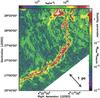Fig. 2 High-resolution (18.2′′) column density map of the Taurus B211+L1495 field derived from the Herschel data. The contrast of filamentary structures has been enhanced using a curvelet transform (cf. Starck et al. 2003). Given the typical width ~0.1 pc of the filaments (Arzoumanian et al. 2011), this map is approximately equivalent to a map of mass per unit length along the filaments. The color bar on the right shows a line-mass scale in units of the thermal critical line mass of Inutsuka & Miyama (1997), which we estimate to be accurate to better than a factor of ~2 according to a detailed analysis of the radial profiles of the filaments (Arzoumanian et al., in prep.). Note that the main B211 filament is thermally supercritical, while the mass per unit length of the faint striations is an order of magnitude below the critical value.

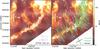Fig. 3 a)Herschel/SPIRE 250 μm image of the B211/B213/L1495 region in Taurus. The light blue and purple curves show the crests of the B213 and B211 segments of the whole filament discussed in this paper, respectively. b) Display of optical and infrared polarization vectors from Heyer et al. (2008), Heiles (2000), and Chapman et al. (2011) tracing the magnetic field orientation in the B211/L1495 region, overlaid on our Herschel/SPIRE 250 μm image. The plane-of-the-sky projection of the magnetic field appears to be oriented perpendicular to the B211/B213 filament and roughly aligned with the general direction of the striations overlaid in blue. The green, blue, and black segments in the lower right corner represent the average position angles of the polarization vectors, low-density striations, and B211 filament, respectively.

3. Analysis of the filamentary structure

In order to facilitate the visualization of individual filaments, we performed a “morphological component analysis” (MCA) decomposition of the Herschel column density map on a basis of curvelets and wavelets (e.g., Starck et al. 2003, 2004). The decomposition was made on 6 scales and 100 iterations were used¹. The map corresponding to the sum of all 6 curvelet components, shown in Fig. 2, provides a high-contrast view of the filaments after subtraction of the non-filamentary background and most of the compact cores. Figure 2 shows that the B211 filament is surrounded by a large number of lower-density filaments or striations which are oriented roughly perpendicular to the main filament. It is important to stress that the striations can also be seen in the original maps (cf. Figs. 1a and 3a) and that the curvelet transform was merely used to enhance their contrast. Some of these striations are also visible in the ¹²CO(1–0) and ¹³CO(1–0) maps of Goldsmith et al. (2008) at 45′′ resolution. Following André et al. (2010), the column density map of Fig. 2 was also converted to an approximate map of mass per unit length along the filaments by multiplying the local column density by the characteristic filament width of 0.1 pc (see color scale on the right of Fig. 2). It can be seen in Fig. 2 that the mass per unit length of the main B211 filament exceeds the thermal value of the critical line mass, ${\mathit{M}}_{\mathrm{line}\mathit{,}\mathrm{crit}}\mathrm{=}\mathrm{2}\hspace{0.17em}{\mathit{c}}_{\mathrm{s}}^{\mathrm{2}}\mathit{/}\mathit{G}$, while the mass per unit length of the striations is an order of magnitude below the critical value. Assuming that the non-thermal component of the velocity dispersion inside the filaments is small compared to the sound speed, as suggested by the results of millimeter line observations (see Hacar & Tafalla 2011, for the L1517 filament and Arzoumanian et al., in prep.) we tentatively conclude that the whole B211 filament is gravitationally unstable, while the perpendicular striations are not.

3.1. A bimodal distribution of filament orientations

To analyze the distribution of filament orientations in a quantitative manner, we applied the DisPerSE algorithm (Sousbie 2011) to the original column density map (Fig. 1a), in order to produce a census of filaments and to trace the locations of their crests. DisPerSE is a general method based on principles of computational topology and it has already been used successfully to trace the filamentary structure in Herschel images of star-forming clouds (e.g., Arzoumanian et al. 2011; Hill et al. 2011; Peretto et al. 2012; Schneider et al. 2012). Using DisPerSE with a relative “persistence” threshold of 10²¹ cm^-2 (~5σ in the map – see Sousbie 2011 for the formal definition of “persistence”) and an absolute column density threshold of 1–2 × 10²¹ cm^-2, we could trace the crests of the B211 filament and 44 lower density filamentary structures (see Fig. 3). Due to differing background levels on either side of the B211/3 filament (see Fig. 1a), we adopted different column density thresholds on the north-eastern side (2 × 10²¹ cm^-2) and south-western side (10²¹ cm^-2). The results of DisPerSE were also visually inspected in both the original and the curvelet column density map, and a few doubtful features discarded. The mean orientation or position angle of each filament was then calculated from its crest (see Appendix A of Peretto et al. 2012, for details). Figure 4 shows the resulting histogram of position angles. In this histogram, the low-density striations are concentrated near a position angle of 34° ± 13°, which is almost orthogonal to the B211 filament (PA = 118° ± 20°). Interestingly, the position-angle distribution of available optical polarization vectors (Heiles 2000; Heyer et al. 2008), which trace the local direction of the magnetic field projected onto the plane-of-sky, is centered on PA = 26° ± 18° and thus very similar to the orientation distribution of the low-density striations (see Fig. 4). Figure 3b further illustrates that the low-density striations are roughly parallel to the B-field polarization vectors and perpendicular to the B211 filament.

3.2. Density and temperature structure of the B211 filament

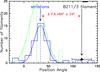Fig. 4 Histogram of orientations for the low-density striations identified with DisPerSE in the B211+L1495 field (displayed in blue). The position-angle distribution of available optical polarization (Heyer et al. 2008, Heiles 2000) and infrared vectors (Chapman et al. 2011) are also shown (green dashed histogram). Gaussian fits to these distributions are superimposed, indicating a peak position angle of 34° ± 13° for the striations and 26 ° ± 18° for the B-field polarization vectors. The B211 filament has a mean position angle of 118° ± 20° (black triangle and horizontal error bar) and is thus roughly perpendicular to both the low-density striations and the local direction of the magnetic field.

Using the original column density and temperature maps derived from the Herschel data (see Appendix A), we produced radial column density and temperature profiles for the B211 filament, following the same procedure as Arzoumanian et al. (2011) for IC5146. We first determined the direction of the local tangent for each pixel along the crest of the B211 filament as traced by DisPerSE. For each pixel, we then derived one temperature profile and one column density profile in the direction perpendicular to the local tangent. Finally, by averaging all individual cuts along the crest, we obtained a mean column density and a mean temperature profile for the B211 filament (Fig. 5).

To characterize the resulting column density profile we made use of an analytical model of an idealized cylindrical filament. This model features a dense, flat inner portion and approaches a power-law behavior at large radii. Analytically, it is described by a Plummer-like function of the form (cf. Nutter et al. 2008; Arzoumanian et al. 2011): $\begin{array}{ccc}{\mathit{\rho }}_{\mathrm{p}}\mathrm{\left(}\mathit{r}\mathrm{\right)}\mathrm{=}\frac{{\mathit{\rho }}_{\mathrm{c}}}{{\mathrm{[}\mathrm{1}\mathrm{+}{\mathrm{(}{\mathit{r}\mathit{/}{\mathit{R}}_{\mathrm{flat}}}^{\mathrm{)}}}^{\mathrm{2}}\mathrm{]}}^{\mathit{p}\mathit{/}\mathrm{2}}}\mathrm{-}\mathrm{\to }{\mathrm{\Sigma }}_{\mathrm{p}}\mathrm{\left(}\mathit{r}\mathrm{\right)}\mathrm{=}{\mathit{A}}_{\mathrm{p}}\hspace{0.17em}\frac{{\mathit{\rho }}_{\mathrm{c}}{\mathit{R}}_{\mathrm{flat}}}{{\mathrm{[}\mathrm{1}\mathrm{+}{\mathrm{(}{\mathit{r}\mathit{/}{\mathit{R}}_{\mathrm{flat}}}^{\mathrm{)}}}^{\mathrm{2}}\mathrm{]}}^{\frac{\mathit{p}\mathrm{-}\mathrm{1}}{\mathrm{2}}}}\mathit{,}& & \end{array}$where ρ_c is the central density of the filament, R_flat is the radius of the flat inner region, p is the power-law exponent at large radii (r ≫ R_flat), ${\mathit{A}}_{\mathrm{p}}\mathrm{=}\frac{\mathrm{1}}{\cos \hspace{0.17em}\mathit{i}}\mathrm{\times }\mathrm{B}{}^{\mathrm{(}}\frac{\mathrm{1}}{\mathrm{2}}\mathit{,}{\frac{\mathrm{p}\mathrm{-}\mathrm{1}}{\mathrm{2}}}^{\mathrm{)}}$ is a finite constant factor (for p > 1) that takes into account the filament’s inclination angle to the plane of the sky (here assumed to be i = 0°), and B represents the Euler beta function (cf. Casali 1986). The density structure of an isothermal gas cylinder in hydrostatic equilibrium follows Eq. (1) with p = 4 (Ostriker 1964).

According to the best-fit model of B211 (cf. Fig. 5a), the diameter of the flat inner portion is 2  R_flat = 0.07 ± 0.02 pc, which is well resolved compared to the 0.012 pc (or 18.2′′) resolution of the column density map. The power-law regime at large radii is ρ ∝ r^{−2.0± 0.4}, which is significantly shallower than the steep ρ ∝ r^-4 profile expected for unmagnetized isothermal filaments but would be consistent with models of isothermal equilibrium filaments threaded by helical magnetic fields (Fiege & Pudritz 2000). Note that our results for the density profile of the B211 filament (e.g. mean deconvolved FWHM width ~0.09 ± 0.02 pc) agree with the characteristic width ~0.1 pc found by Arzoumanian et al. (2011) for filaments in IC5146, Aquila, Polaris, and very similar to the findings of Malinen et al. (2012) for the TMC-1 filament (also known as the Bull’s tail – Nutter et al. 2008). Malinen et al. derived p ≈ 2.3 and 2   R_flat ≈ 0.09 pc, also based on Herschel data from the HGBS. In addition, the dust temperature profile of the B211 filament shows a pronounced temperature drop toward the center (Fig. 5b), which suggests that the gas is not strictly isothermal².

A reasonably good model for the structure of the B211 filament is obtained by considering similarity solutions for the collapse of an infinite cylinder obeying a polytropic (non-isothermal) equation of state of the form P ∝ ρ^γ with γ ≲ 1. Kawachi & Hanawa (1998) have shown that the outer density profile of such a collapsing cylinder approaches the power law $\mathit{\rho }\mathrm{\propto }{\mathit{r}}^{\mathrm{-}\frac{\mathrm{2}}{\mathrm{2}\mathrm{-}\mathit{\gamma }}}$. For γ values close to unity, the model column density profile thus approaches ρ ∝ r^-2 at large radii, which is consistent with the observed profile of the B211 filament. The best Plummer model derived above for the density profile (ρ_p(r) – Fig. 5a) can be used to estimate the γ value which leads to the best fit to the observed dust temperature profile² under the polytropic assumption [T(r) ∝ ρ_p(r)^(γ−1)]. The resulting model fit, overlaid in red in Fig. 5b, has γ = 0.97 ± 0.01 < 1, corresponding to ρ ∝ r^{− 1.96    ±    0.02} at large radii for a self-similar, not strictly isothermal collapsing cylinder.

4. Discussion: contraction and accretion in B211?

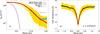Fig. 5 a) Mean radial column density profile observed perpendicular to the B211 filament and displayed in log-log format, for both the northern (blue curve) and the southern part (red curve) of the filament. The yellow area shows the (±1σ) dispersion of the distribution of radial profiles along the filament. The inner solid purple curve shows the effective 18.2′′ HPBW resolution (0.012 pc at 140 pc) of the column density map (online Fig. 1 – see Appendix A for details) used to construct the profile. The northern and southern column density profiles are very similar up to r ~ 0.4 pc (vertical dashed line) and differ significantly only for r > 0.4 pc, due to different background levels on either side of the filament. The dashed black curve shows the best-fit Plummer model (convolved with the 18.2′′ beam) described by Eq. (1) with p = 2.0 ± 0.4 and Rflat = 0.03 ± 0.01 pc for r ≤ 0.4 pc, and including a separate linear baseline on each side representing the background for r > 0.4 pc (see Eq. (B1) in Appendix B, for details). The dashed curve in light green shows a Gaussian fit to the central part of the profile (mean deconvolved FWHM width ~0.09 ± 0.02 pc). b) Mean dust temperature profile measured perpendicular to the B211 filament and displayed using a linear scale (black curve). The solid red curve shows the best model temperature profile obtained by assuming that the filament has a density profile given by the Plummer model shown in a) and obeys a polytropic equation of state, $\mathit{P}\mathrm{\propto }{\mathit{\rho }}_{\mathrm{p}}^{\mathit{\gamma }}$, and thus T(r) ∝ ρp(r)(γ − 1). This best fit has γ = 0.97 ± 0.01.

The results presented in this paper reveal the density and temperature structure of the Taurus B211 filament with unprecedented detail. The shape of the column density profile derived for the B211 filament, with a well-defined power-law regime at large radii (see Fig. 5a), and the high column density contrast over the surrounding background (a factor ~10–20, implying a density contrast ~100–400) strongly suggest that the main filament has undergone gravitational contraction. This is also consistent with the supercritical mass per unit length measured for the B211 filament (M_line ≈ 54  M_⊙/pc), which suggests that the filament is unstable to both radial contraction and fragmentation into cores (e.g., Inutsuka & Miyama 1997; Pon et al. 2011). Observations confirm that the B211 filament has indeed fragmented, leading to the formation of several prestellar cores (e.g., Onishi et al. 2002) and protostars (e.g., Motte & André 2001; Rebull et al. 2010) along its length.

The orientation alignment of the striations with optical polarization vectors suggests that the magnetic field plays an important role in shaping the morphology of the filamentary structure in this part of Taurus. Earlier studies, using similar polarization observations of background stars, already pointed out that the structure of the Taurus cloud was strongly correlated with the morphology of the ambient magnetic field (e.g. Heyer et al. 2008; Chapman et al. 2011, and references therein). Using the Chandrasekhar–Fermi method, Chapman et al. (2011) estimated a magnetic field strength of ~25 μG in the B211 area and concluded that the region corresponding to the striations seen here in, e.g., Figs. 2 and 3 was magnetically subcritical.

Theoretical arguments (e.g., Nagai et al. 1998) predict that, in the presence of a “strong” magnetic field, low-density, thermally subcritical filaments such as the striations observed in Taurus should be preferentially oriented parallel to the field lines, while high-density, self-gravitating filaments should be preferentially oriented perpendicular to the field lines. This difference arises because low-density structures which are not held by gravity have a tendency to expand and disperse, while self-gravitating structures have a tendency to contract. In the presence of a magnetic field, motions of slightly ionized gas do not encounter any resistance along the field lines but encounter significant resistance perpendicular to the field lines. Consequently, an initial perturbation in a low-density part of the cloud will tend to expand along the field lines and form an elongated structure or a subcritical “filament” parallel to the field. Conversely, a self-gravitating structure will tend to contract along the field lines, forming a condensed, self-gravitating sheet (cf. Nakamura & Li 2008) which can itself fragment into several supercritical filaments oriented perpendicular to the field (e.g. Nagai et al. 1998). These simple arguments may explain the distribution of filament orientations with two orthogonal groups found in Sect. 3.1 (see Fig. 4). Other regions imaged with Herschel where a similar distribution of filament orientations is observed and a similar mechanism may be at work include the Pipe nebula (Peretto et al. 2012), the Musca cloud (Cox et al. in prep.) and the DR21 ridge in Cygnus X (Schneider et al. 2010; Hennemann et al. 2012).

The morphology of the region with a number of low-density striations parallel to the magnetic field lines, some of them approaching the B211 filament from the side and apparently connected to it (see Fig. 2), is also suggestive of mass accretion along the field lines into the main filament. To test this hypothesis, we assume cylindrical geometry and use the observed mass per unit length M_line to estimate the gravitational acceleration g(R) = 2   GM_line(r < R)/R of a piece of gas in free-fall toward the B211 filament, where R represents radius. The free-fall velocity v_ff of gas initially at rest at a cylindrical radius R_init ~ 2 pc (corresponding to the most distant striations) is estimated to reach v_ff = 2   [GM_line   ln(R_init/R)]^1/2 ≈ 1.1 km s^-1 when the material reaches the outer radius R ~ 0.4 pc of the B211 filament. This free-fall estimate is an upper limit since it neglects any form of support against gravity. A more conservative estimate can be obtained by considering the similarity solution found by Kawachi & Hanawa (1998) for the gravitational collapse of a cylindrical filament supported by a polytropic pressure gradient with γ ≲ 1. In this model, the radial infall velocity in the outer parts of the collapsing filament is expected to be v_inf ~ 0.6–1 km s^-1 when γ = 0.9–0.999 and the gas temperature is ~10 K (see Figs. 4 and 6 of Kawachi & Hanawa). The above two velocity estimates can be compared with the kinematical constraints provided by the ¹²CO(1–0) observations of Goldsmith et al. (2008). It can be seen in online Fig. 6 that there is an average velocity difference of ~1 km s^-1 between the redshifted CO emission observed at V_LSR ~ 7 km s^-1 to the north-east and the B211 filament which has V_LSR ~ 6 km s^-1. Likewise, there is an average difference of ~1 km s^-1 between the blueshifted CO emission observed at V_LSR ~ 5 km s^-1 to the south-west and the B211 filament. Although projection effects may somewhat increase the magnitude of the intrinsic velocity difference, we conclude that there is good qualitative agreement between the estimated inflow velocity in the striations and the ¹²CO observational constraints. Considering these velocities, the current mass accretion rate onto the 4-pc-long filament (total mass of ~220  M_⊙) is estimated to be on the order of M_line = ρ_p(R)    ×    v_inf    ×    2πR ≈ 27–50 M_⊙/pc/Myr, where ρ_p(R) corresponds to the density of the best-fit Plummer model at the filament outer radius R = 0.4 pc. This would mean that it would take ~1–2 Myr for the central filament to form at the current accretion rate and ~0.8–1.5 Myr for the total mass of the striations (~150  M_⊙) to be accreted. The available observational evidence therefore lends some credence to the view that the B211 filament is radially contracting toward its long axis, while at the same time accreting additional ambient material through the striations.

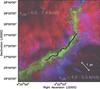Fig. 6 CO emission observed toward and around the B211 filament (Goldsmith et al. 2008). Redshifted 12CO(1–0) emission integrated from VLSR = 6.6 km s-1 to VLSR = 7.4 km s-1 is displayed in red and mostly seen to the north-east of the B211 filament. Blueshifted 12CO(1–0) emission integrated from VLSR = 4.2 km s-1 to VLSR = 5.5 km s-1 is displayed in blue and mostly seen to the south-west of the filament. The main body of the B211 filament, displayed in green, corresponds to the 13CO(1–0) emission detected between VLSR = 5.6 km s-1 to VLSR = 6.4 km s-1. Both 12CO(1–0) and 13CO(1–0) maps have a spectral resolution of ~0.2 km s-1.

Online material

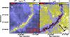Fig. 1 a) High-resolution (18.2′′) column density map of the Taurus B211/B213 region (in units of NH2 cm-2) derived from Herschel data as explained in Appendix A. b) Dust temperature map of the Taurus B211/B213 region (in K) derived at 36.3′′ from Herschel data. Comparison of the two panels shows how dust temperature and column density are anti-correlated.

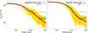Fig. 7 Mean radial column density profiles of the B213 (left) and B211 (right) segments of the filament for both the north-eastern (in blue) and south-western (in red) sides. In both panels, the black dashed curve represents the mean of the best-fit Plummer models to the north-eastern and south-western profiles, truncated at r = 0.4 pc where the backgrounds start to diverge significantly between the two sides. The crests defining the B213 and B211 segments considered here can be seen in Fig. 3a. The B213 segment has a slightly shallower profile (p ≈ 1.7) and a smaller flat inner radius (Rflat ≈ 0.025 pc) than the B211 segment (p ≈ 2.6 and Rflat ≈ 0.06 pc). The detailed parameters of the model fits are given in Table B.1.

Appendix A: Derivation of a high-resolution (18.2′′) column density map

The procedure employed here to construct a column density map at the 18.2′′ resolution of the SPIRE 250 μm data for the B211+L1495 region is consistent with, but represents an improvement over, the method used in earlier HGBS papers to derive column density maps at the 36.3′′ resolution of SPIRE 500 μm observations. Following the spirit of a multi-scale decomposition of the data (cf. Starck et al. 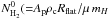2004), the gas surface density distribution of the region, smoothed to the resolution of the SPIRE 250 μm observations, may be expressed as a sum of three terms: $\begin{array}{ccc}{\mathrm{\Sigma }}_{\mathrm{250}}\mathrm{=}{\mathrm{\Sigma }}_{\mathrm{500}}\mathrm{+}\mathrm{(}{\mathrm{\Sigma }}_{\mathrm{350}}\mathrm{-}{\mathrm{\Sigma }}_{\mathrm{500}}\mathrm{)}\mathrm{+}\mathrm{(}{\mathrm{\Sigma }}_{\mathrm{250}}\mathrm{-}{\mathrm{\Sigma }}_{\mathrm{350}}\mathrm{)}\mathit{.}& & \end{array}$(A.1)In the above equation, Σ₅₀₀, Σ₃₅₀, and Σ₂₅₀ represent smoothed versions of the intrinsic gas surface density distribution Σ after convolution with the SPIRE beam at 500 μm, 350 μm, and 250 μm, respectively, i.e.: Σ₅₀₀ = Σ∗B₅₀₀, Σ₃₅₀ = Σ∗B₃₅₀, and Σ₂₅₀ = Σ∗B₂₅₀.

The first term of Eq. (A.1) is simply the surface density distribution smoothed to the resolution of the SPIRE 500 μm data. An estimate, , of this term can be derived from the Herschel data using the same procedure as in earlier HGBS papers (e.g. Könyves et al. 2010). Briefly, the Herschel images including the zero-level offsets estimated from IRAS and Planck (cf. Bernard et al. 2010) are first smoothed to the 500 μm resolution (36.3′′) and reprojected onto the same grid. An optically thin graybody function of the form I_ν = B_ν(T_d)   κ_ν   Σ, where I_ν is the observed surface brightness at frequency ν, and κ_ν is the dust opacity per unit (dust+gas) mass, is then fitted to the spectral energy distributions (SEDs) observed with Herschel between 160 μm and 500 μm, on a pixel-by-pixel basis (four SED data points per pixel). This makes it possible to estimate the best-fit value and T_d,500(x,y) at each pixel position (x,y). The following dust opacity law, very similar to that advocated by Hildebrand (1983) at submillimeter wavelengths, is assumed: κ_ν = 0.1 × (ν/1000  GHz)^β = 0.1 × (300  μm/λ)^β cm²/g, with β = 2.

The second term of Eq. (A.1) may be written as Σ₃₅₀ − Σ₃₅₀ ∗ G_{500_350}, where G_{500_350} is a circular Gaussian with full width at half maximum (FWHM) 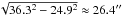$\sqrt{{\mathrm{36.3}}^{\mathrm{2}}\mathrm{-}{\mathrm{24.9}}^{\mathrm{2}}}\mathrm{\approx }\mathrm{26.4}″$. (To first order, the SPIRE beam at 500 μm is a smoothed version of the SPIRE beam at 350 μm, i.e., B₅₀₀ = B₃₅₀ ∗ G_{500_350}). The second term of Eq. (A.1) may thus be viewed as a term adding information on spatial scales accessible to SPIRE observations at 350  μm, but not to SPIRE observations at 500  μm. In practice, one can derive and estimate of Σ₃₅₀ in a manner similar to , through pixel-by-pixel SED fitting to three Herschel data points between 160 μm and 350 μm (i.e., ignoring the lower resolution 500 μm data point). An estimate of the second term of Eq. (A.1) can then be obtained by subtracting a smoothed version of (i.e., ) to itself, i.e., by removing low spatial frequency information from .

Likewise, the third term of Eq. (A.1) may be written as Σ₂₅₀ − Σ₂₅₀ ∗ G_{350_250}, where G_{350_250} is a circular Gaussian with $\mathit{FWHM}\sqrt{{\mathrm{24.9}}^{\mathrm{2}}\mathrm{-}{\mathrm{18.2}}^{\mathrm{2}}}\mathrm{\approx }\mathrm{17.0}″$, and may be understood as a term adding information on spatial scales only accessible to Herschel observations at wavelengths ≤250 μm. In order to derive an estimate of Σ₂₅₀ on the right-hand side of Eq. (A.1), we first smooth the PACS 160 μm map to the 18.2′′ resolution of the SPIRE 250 μm map and then derive a color temperature map between 160 μm and 250 μm from the observed I_250  μm(x,y)/I_160  μm(x,y) intensity ratio at each pixel (x,y). The SPIRE 250 μm map is converted into a gas surface density map (), assuming optically thin dust emission at the temperature given by the color temperature map and a dust opacity at 250 μm κ_250  μm = 0.1 × (300/250)² cm²/g. An estimate of the third term of Eq. (A.1) can then be obtained by subtracting a smoothed version of (i.e., ) to itself, i.e., by removing low spatial frequency information from .

Our final estimate $\begin{array}{c}{\mathrm{˜}}_{}\\ {\mathrm{\Sigma }}_{\mathrm{250}}\end{array}$ of the gas surface density distribution at 18.2′′ resolution is produced by adding up the above estimates of the three terms on the right-hand side of Eq. (A.1): $\begin{array}{ccc}\begin{array}{c}\mathrm{˜}\\ {\mathrm{\Sigma }}_{\mathrm{250}}\end{array}& \mathrm{=}& \mathrm{\Sigma ̅}\mathrm{500}\mathrm{+}\left(\mathrm{\Sigma ̅}\mathrm{350}\mathrm{-}\mathrm{\Sigma ̅}\mathrm{350}\mathrm{\ast }{\mathit{G}}_{\mathrm{500}\mathrm{\_}\mathrm{350}}\right)\\ & & \mathrm{+}\hspace{0.17em}\left(\mathrm{\Sigma ̅}\mathrm{250}\mathrm{-}\mathrm{\Sigma ̅}\mathrm{250}\mathrm{\ast }{\mathit{G}}_{\mathrm{350}\mathrm{\_}\mathrm{250}}\right)\mathit{.}\end{array}$(A.2)The resulting 18.2′′-resolution column density map $\begin{array}{c}{\mathrm{˜}}_{}\\ {\mathit{N}}_{{\mathrm{H}}_{\mathrm{2}}}\end{array}$ for the B211+L1495 region is displayed in online Fig. 1a in units of mean molecules per cm², where $\begin{array}{c}{}_{\mathrm{˜}}\\ {\mathrm{\Sigma }}_{\mathrm{250}}\end{array}\mathrm{=}\mathit{\mu }\hspace{0.17em}{\mathrm{m}}_{\mathrm{H}}\hspace{0.17em}\begin{array}{c}{}_{\mathrm{˜}}\\ {\mathit{N}}_{{\mathrm{H}}_{\mathrm{2}}}\end{array}$ and μ = 2.33 is the mean molecular weight. Although this high-resolution map is somewhat noisier than its 36.3′′-resolution counterpart (corresponding to ) and has lower signal-to-noise ratio than the SPIRE 250 μm image (cf. Fig. 3), due to additional noise coming from the second and third terms of Eq. (A.1), the quality and dynamic range of the Herschel data are such that the result provides a very useful estimate of the column density distribution in B211+L1495 with a factor of 2 better resolution than standard column density maps derived so far from Herschel observations.

Because the higher-resolution terms in Eq. (A.1) are derived using fewer and fewer SED data points to estimate the effective dust temperature T_d for each line of sight, the high-resolution column density map is also somewhat less reliable than the standard 36.3′′-resolution column density map (corresponding to ). To evaluate the reliability of the and maps entering the calculation of $\begin{array}{c}{\mathrm{˜}}_{}\\ {\mathrm{\Sigma }}_{\mathrm{250}}\end{array}$ (cf. Eq. (A.2)) and derived using only three and two SED data points per position, respectively, we made the following tests in the case of the Taurus B211/B213+L1495 data. First, from the Herschel 160 μm to 350 μm images smoothed to the 500 μm resolution, we derived a dust temperature map ${\mathit{T}}_{\mathrm{d}\mathit{,}\mathrm{350}}^{\mathrm{500}}$ and a gas surface density map $\mathrm{\Sigma ̅}\begin{array}{c}\mathrm{500}\\ \mathrm{350}\end{array}$ using the three Herschel data points between 160 μm and 350 μm and compared these maps to the maps T_d,500 and derived at the same resolution using four SED data points per position. In the case of the Taurus data, the ${\mathit{T}}_{\mathrm{d}\mathit{,}\mathrm{350}}^{\mathrm{500}}$ map agrees with the T_d,500 map to better than 0.15 K on average (and better than 0.8 K everywhere) and $\mathrm{\Sigma ̅}\begin{array}{c}\mathrm{500}\\ \mathrm{350}\end{array}$ agrees with to better than 4% on average (and better than 25% everywhere). Likewise, using the Herschel 160 μm and 250 μm images smoothed to the 500 μm resolution, we derived a color temperature map ${\mathit{T}}_{\mathrm{d}\mathit{,}\mathrm{250}}^{\mathrm{500}}$ and a gas surface density map $\mathrm{\Sigma ̅}\begin{array}{c}\mathrm{500}\\ \mathrm{250}\end{array}$ in the same way as we calculated above and then compared these maps to the T_d,500 and maps. The ${\mathit{T}}_{\mathrm{d}\mathit{,}\mathrm{250}}^{\mathrm{500}}$ map agrees with the T_d,500 map to better than 0.15 K on average (and better than 1.2 K everywhere) and $\mathrm{\Sigma ̅}\begin{array}{c}\mathrm{500}\\ \mathrm{250}\end{array}$ agrees with to better than 3% on average (and better than 30% everywhere)³. Finally, to test the robustness of the 18.2′′-resolution column density map $\begin{array}{c}{\mathrm{˜}}_{}\\ {\mathrm{\Sigma }}_{\mathrm{250}}\end{array}$, we smoothed it to the 36.3′′ resolution of the standard column density map and inspected the ratio map between the two, which has a mean value of 1.00 and a standard deviation of 0.04. Within the region covered by both PACS and SPIRE, the smoothed version of $\begin{array}{c}{\mathrm{˜}}_{}\\ {\mathrm{\Sigma }}_{\mathrm{250}}\end{array}$ agrees with to better than 10%.

Appendix B: Details of the procedure used e to fit the column density profile of the B211/B213 filament

The fitting analysis of the observed column density profile (Sect. 3.2 and Fig. 5) was performed using the non-linear least-squares fitting IDL procedure MPFIT (Markwardt, C. B. 2008 – http://purl.com/net/mpfit). In addition to the Plummer-like cylindrical model filament corresponding to Eq. (1) with three free parameters, the background gas was represented by two separate linear baselines on either side of the filament.

Each side was fitted independently with the following model function (convolved with the beam): $\begin{array}{ccc}{\mathrm{\Sigma }}_{\mathrm{p}}\mathrm{\left(}\mathit{r}\mathrm{\right)}\mathit{/}\mathit{\mu }\hspace{0.17em}{\mathit{m}}_{\mathit{H}}\mathrm{=}\hspace{0.17em}\frac{{\mathit{N}}_{{\mathrm{H}}_{\mathrm{2}}}^{\mathrm{0}}}{{\mathrm{[}\mathrm{1}\mathrm{+}{\mathrm{(}{\mathit{r}\mathit{/}{\mathit{R}}_{\mathrm{flat}}}^{\mathrm{)}}}^{\mathrm{2}}\mathrm{]}}^{\frac{\mathit{p}\mathrm{-}\mathrm{1}}{\mathrm{2}}}}\mathrm{+}\mathit{Bkg}\mathrm{\left[}\mathrm{1}\mathrm{\right]}\mathit{r}\mathrm{+}\mathit{Bkg}\mathrm{\left[}\mathrm{0}\mathrm{\right]}\mathit{,}& & \end{array}$(B.1)where ${\mathit{N}}_{{\mathrm{H}}_{\mathrm{2}}}^{\mathrm{0}}\mathrm{(}\mathrm{=}{\mathit{A}}_{\mathrm{p}}{\mathit{\rho }}_{\mathrm{c}}{\mathit{R}}_{\mathrm{flat}}\mathit{/}\mathit{\mu }\hspace{0.17em}{\mathit{m}}_{\mathit{H}}$), R_flat, p, Bkg[1], and Bkg[0] were treated as five free parameters. Bkg[1] and Bkg[0] are two parameters which describe the local background cloud gas. The results of these model fits are given in Table B.1.1 for both the north-eastern and the south-western side of the B211/B213 filament considered as a whole (see Fig. 5a), as well as for the B211 and the B213 segment of the whole filament (see online Fig. 7). Due to differing background levels on either side of the filament, fitting the two sides of the filament separately gives better results than a single fit to both sides simultaneously.

Acknowledgments

P.P. is funded by the Fundação para a Ciência e a Tecnologia (Portugal). We are grateful to Paul Goldsmith for making the FCRAO CO(1–0) data of the B211/L1495 region available to us. We thank Shu-ichiro Inutsuka and Fumitaka Nakamura for insightful discussions about filaments. D.E. and K.L.J.R. are funded by an ASI fellowship under contract number I/005/11/0. SPIRE has been developed by a consortium of institutes led by Cardiff Univ. (UK) and including Univ. Lethbridge (Canada); NAOC (China); CEA, LAM (France); IFSI, Univ. Padua (Italy); IAC (Spain); Stockholm Observatory (Sweden); Imperial College London, RAL, UCL-MSSL, UKATC, Univ. Sussex (UK); Caltech, JPL, NHSC, Univ. Colorado (USA). This development has been supported by national funding agencies: CSA (Canada); NAOC (China); CEA, CNES, CNRS (France); ASI (Italy); MCINN (Spain); SNSB (Sweden); STFC (UK); and NASA (USA). PACS has been developed by a consortium of institutes led by MPE (Germany) and including UVIE (Austria); KUL, CSL, IMEC (Belgium); CEA, OAMP (France); MPIA (Germany); IFSI, OAP/AOT, OAA/CAISMI, LENS, SISSA (Italy); IAC (Spain). This development has been supported by the funding agencies BMVIT (Austria), ESA-PRODEX (Belgium), CEA/CNES (France), DLR (Germany), ASI (Italy), and CICT/MCT (Spain).

References

All Tables

All Figures

Fig. 2 High-resolution (18.2′′) column density map of the Taurus B211+L1495 field derived from the Herschel data. The contrast of filamentary structures has been enhanced using a curvelet transform (cf. Starck et al. 2003). Given the typical width ~0.1 pc of the filaments (Arzoumanian et al. 2011), this map is approximately equivalent to a map of mass per unit length along the filaments. The color bar on the right shows a line-mass scale in units of the thermal critical line mass of Inutsuka & Miyama (1997), which we estimate to be accurate to better than a factor of ~2 according to a detailed analysis of the radial profiles of the filaments (Arzoumanian et al., in prep.). Note that the main B211 filament is thermally supercritical, while the mass per unit length of the faint striations is an order of magnitude below the critical value.

In the text

Fig. 3 a)Herschel/SPIRE 250 μm image of the B211/B213/L1495 region in Taurus. The light blue and purple curves show the crests of the B213 and B211 segments of the whole filament discussed in this paper, respectively. b) Display of optical and infrared polarization vectors from Heyer et al. (2008), Heiles (2000), and Chapman et al. (2011) tracing the magnetic field orientation in the B211/L1495 region, overlaid on our Herschel/SPIRE 250 μm image. The plane-of-the-sky projection of the magnetic field appears to be oriented perpendicular to the B211/B213 filament and roughly aligned with the general direction of the striations overlaid in blue. The green, blue, and black segments in the lower right corner represent the average position angles of the polarization vectors, low-density striations, and B211 filament, respectively.

In the text

Fig. 4 Histogram of orientations for the low-density striations identified with DisPerSE in the B211+L1495 field (displayed in blue). The position-angle distribution of available optical polarization (Heyer et al. 2008, Heiles 2000) and infrared vectors (Chapman et al. 2011) are also shown (green dashed histogram). Gaussian fits to these distributions are superimposed, indicating a peak position angle of 34° ± 13° for the striations and 26 ° ± 18° for the B-field polarization vectors. The B211 filament has a mean position angle of 118° ± 20° (black triangle and horizontal error bar) and is thus roughly perpendicular to both the low-density striations and the local direction of the magnetic field.

In the text

Fig. 5 a) Mean radial column density profile observed perpendicular to the B211 filament and displayed in log-log format, for both the northern (blue curve) and the southern part (red curve) of the filament. The yellow area shows the (±1σ) dispersion of the distribution of radial profiles along the filament. The inner solid purple curve shows the effective 18.2′′ HPBW resolution (0.012 pc at 140 pc) of the column density map (online Fig. 1 – see Appendix A for details) used to construct the profile. The northern and southern column density profiles are very similar up to r ~ 0.4 pc (vertical dashed line) and differ significantly only for r > 0.4 pc, due to different background levels on either side of the filament. The dashed black curve shows the best-fit Plummer model (convolved with the 18.2′′ beam) described by Eq. (1) with p = 2.0 ± 0.4 and Rflat = 0.03 ± 0.01 pc for r ≤ 0.4 pc, and including a separate linear baseline on each side representing the background for r > 0.4 pc (see Eq. (B1) in Appendix B, for details). The dashed curve in light green shows a Gaussian fit to the central part of the profile (mean deconvolved FWHM width ~0.09 ± 0.02 pc). b) Mean dust temperature profile measured perpendicular to the B211 filament and displayed using a linear scale (black curve). The solid red curve shows the best model temperature profile obtained by assuming that the filament has a density profile given by the Plummer model shown in a) and obeys a polytropic equation of state, $\mathit{P}\mathrm{\propto }{\mathit{\rho }}_{\mathrm{p}}^{\mathit{\gamma }}$, and thus T(r) ∝ ρp(r)(γ − 1). This best fit has γ = 0.97 ± 0.01.

In the text

Fig. 6 CO emission observed toward and around the B211 filament (Goldsmith et al. 2008). Redshifted 12CO(1–0) emission integrated from VLSR = 6.6 km s-1 to VLSR = 7.4 km s-1 is displayed in red and mostly seen to the north-east of the B211 filament. Blueshifted 12CO(1–0) emission integrated from VLSR = 4.2 km s-1 to VLSR = 5.5 km s-1 is displayed in blue and mostly seen to the south-west of the filament. The main body of the B211 filament, displayed in green, corresponds to the 13CO(1–0) emission detected between VLSR = 5.6 km s-1 to VLSR = 6.4 km s-1. Both 12CO(1–0) and 13CO(1–0) maps have a spectral resolution of ~0.2 km s-1.

In the text

	Fig. 1 a) High-resolution (18.2′′) column density map of the Taurus B211/B213 region (in units of NH2 cm-2) derived from Herschel data as explained in Appendix A. b) Dust temperature map of the Taurus B211/B213 region (in K) derived at 36.3′′ from Herschel data. Comparison of the two panels shows how dust temperature and column density are anti-correlated.
In the text

Fig. 7 Mean radial column density profiles of the B213 (left) and B211 (right) segments of the filament for both the north-eastern (in blue) and south-western (in red) sides. In both panels, the black dashed curve represents the mean of the best-fit Plummer models to the north-eastern and south-western profiles, truncated at r = 0.4 pc where the backgrounds start to diverge significantly between the two sides. The crests defining the B213 and B211 segments considered here can be seen in Fig. 3a. The B213 segment has a slightly shallower profile (p ≈ 1.7) and a smaller flat inner radius (Rflat ≈ 0.025 pc) than the B211 segment (p ≈ 2.6 and Rflat ≈ 0.06 pc). The detailed parameters of the model fits are given in Table B.1.

In the text

References

- André, P., Men’shchikov, A., Bontemps, S., et al. 2010, A&A, 518, L102 [NASA ADS] [CrossRef] [EDP Sciences] [Google Scholar]
- André, P., Men’shchikov, A., Könyves, V., & Arzoumanian, D. 2011, in Computational Star Formation, eds. J. Alves, B. G. Elmegreen, J. M. Girart, & V. Trimble, IAU Symp., 270, 255 [Google Scholar]
- Arzoumanian, D., André, P., Didelon, P., et al. 2011, A&A, 529, L6 [Google Scholar]
- Bernard, J.-P., Paradis, D., Marshall, D. J., et al. 2010, A&A, 518, L88 [NASA ADS] [CrossRef] [EDP Sciences] [Google Scholar]
- Casali, M. M. 1986, MNRAS, 223, 341 [NASA ADS] [Google Scholar]
- Chapman, N. L., Goldsmith, P. F., Pineda, J. L., et al. 2011, ApJ, 741, 21 [NASA ADS] [CrossRef] [Google Scholar]
- Elias, J. H. 1978, ApJ, 224, 857 [NASA ADS] [CrossRef] [Google Scholar]
- Falgarone, E., Pety, J., & Hily-Blant, P. 2009, A&A, 507, 355 [NASA ADS] [CrossRef] [EDP Sciences] [Google Scholar]
- Federrath, C., Roman-Duval, J., Klessen, R. S., Schmidt, W., & Mac Low, M. 2010, A&A, 512, A81 [NASA ADS] [CrossRef] [EDP Sciences] [Google Scholar]
- Fischera, J., & Martin, P. G. 2012, A&A, 542, A77 [NASA ADS] [CrossRef] [EDP Sciences] [Google Scholar]
- Galli, D., Walmsley, M., & Gonçalves, J. 2002, A&A, 394, 275 [NASA ADS] [CrossRef] [EDP Sciences] [Google Scholar]
- Goldsmith, P. F., Heyer, M., Narayanan, G., et al. 2008, ApJ, 680, 428 [NASA ADS] [CrossRef] [Google Scholar]
- Goodman, A. A., Barranco, J. A., Wilner, D. J., & Heyer, M. H. 1998, ApJ, 504, 223 [NASA ADS] [CrossRef] [Google Scholar]
- Griffin, M. J., Abergel, A., Abreu, A., et al. 2010, A&A, 518, L3 [Google Scholar]
- Hacar, A., & Tafalla, M. 2011, A&A, 533, A34 [NASA ADS] [CrossRef] [EDP Sciences] [Google Scholar]
- Hartmann, L. 2002, ApJ, 566, L29 [NASA ADS] [CrossRef] [Google Scholar]
- Heiles, C. 2000, AJ, 119, 923 [NASA ADS] [CrossRef] [Google Scholar]
- Hennemann, M., Motte, F., Schneider, N., et al. 2012, A&A, 543, L3 [NASA ADS] [CrossRef] [EDP Sciences] [Google Scholar]
- Heyer, M., Gong, H., Ostriker, E., & Brunt, C. 2008, ApJ, 680, 420 [NASA ADS] [CrossRef] [Google Scholar]
- Hildebrand, R. H. 1983, QJRAS, 24, 267 [NASA ADS] [Google Scholar]
- Hill, T., Motte, F., Didelon, P., et al. 2011, A&A, 533, A94 [NASA ADS] [CrossRef] [EDP Sciences] [Google Scholar]
- Inutsuka, S., & Miyama, S. M. 1997, ApJ, 480, 681 [NASA ADS] [CrossRef] [Google Scholar]
- Kawachi, T., & Hanawa, T. 1998, PASJ, 50, 577 [NASA ADS] [CrossRef] [Google Scholar]
- Kirk, J., Ward-Thompson, D., Palmeirim, P., et al. 2012, MNRAS, submitted [Google Scholar]
- Könyves, V., André, P., Men’shchikov, A., et al. 2010, A&A, 518, L106 [NASA ADS] [CrossRef] [EDP Sciences] [Google Scholar]
- Li, D., & Goldsmith, P. F. 2012, ApJ, 756, 12 [NASA ADS] [CrossRef] [Google Scholar]
- Malinen, J., Juvela, M., Rawlings, M. G., et al. 2012, A&A, 544, A50 [NASA ADS] [CrossRef] [EDP Sciences] [Google Scholar]
- Men’shchikov, A., André, P., Didelon, P., et al. 2010, A&A, 518, L103 [NASA ADS] [CrossRef] [EDP Sciences] [Google Scholar]
- Molinari, S., Swinyard, B., Bally, J., et al. 2010, A&A, 518, L100 [NASA ADS] [CrossRef] [EDP Sciences] [Google Scholar]
- Motte, F., & André, P. 2001, A&A, 365, 440 [NASA ADS] [CrossRef] [EDP Sciences] [Google Scholar]
- Nagai, T., Inutsuka, S.-I., & Miyama, S. M. 1998, ApJ, 506, 306 [NASA ADS] [CrossRef] [Google Scholar]
- Nakamura, F., & Li, Z. 2008, ApJ, 687, 354 [NASA ADS] [CrossRef] [Google Scholar]
- Nutter, D., Kirk, J. M., Stamatellos, D., & Ward-Thompson, D. 2008, MNRAS, 384, 755 [NASA ADS] [CrossRef] [Google Scholar]
- Onishi, T., Mizuno, A., Kawamura, A., Tachihara, K., & Fukui, Y. 2002, ApJ, 575, 950 [NASA ADS] [CrossRef] [Google Scholar]
- Ostriker, J. 1964, ApJ, 140, 1056 [NASA ADS] [CrossRef] [MathSciNet] [Google Scholar]
- Padoan, P., Juvela, M., Goodman, A. A., & Nordlund, Å. 2001, ApJ, 553, 227 [NASA ADS] [CrossRef] [Google Scholar]
- Peretto, N., André, P., Könyves, V., et al. 2012, A&A, 541, A63 [NASA ADS] [CrossRef] [EDP Sciences] [Google Scholar]
- Pilbratt, G. L., Riedinger, J. R., Passvogel, T., et al. 2010, A&A, 518, L1 [CrossRef] [EDP Sciences] [Google Scholar]
- Poglitsch, A., Waelkens, C., Geis, N., et al. 2010, A&A, 518, L2 [NASA ADS] [CrossRef] [EDP Sciences] [Google Scholar]
- Pon, A., Johnstone, D., & Heitsch, F. 2011, ApJ, 740, 88 [NASA ADS] [CrossRef] [Google Scholar]
- Rebull, L. M., Padgett, D. L., McCabe, C.-E., et al. 2010, ApJS, 186, 259 [NASA ADS] [CrossRef] [Google Scholar]
- Roussel, H. 2012 [arXiv:1205.2576] [Google Scholar]
- Schmalzl, M., Kainulainen, J., Quanz, S. P., et al. 2010, ApJ, 725, 1327 [NASA ADS] [CrossRef] [Google Scholar]
- Schneider, S., & Elmegreen, B. G. 1979, ApJS, 41, 87 [NASA ADS] [CrossRef] [Google Scholar]
- Schneider, N., Csengeri, T., Bontemps, S., et al. 2010, A&A, 520, A49 [NASA ADS] [CrossRef] [EDP Sciences] [Google Scholar]
- Schneider, N., Csengeri, T., Hennemann, M., et al. 2012, A&A, 540, L11 [NASA ADS] [CrossRef] [EDP Sciences] [Google Scholar]
- Shu, F. H., Adams, F. C., & Lizano, S. 1987, ARA&A, 25, 23 [Google Scholar]
- Sousbie, T. 2011, MNRAS, 414, 350 [NASA ADS] [CrossRef] [Google Scholar]
- Starck, J. L., Donoho, D. L., & Candès, E. J. 2003, A&A, 398, 785 [NASA ADS] [CrossRef] [EDP Sciences] [Google Scholar]
- Starck, J.-L., Elad, M., & Donoho, D. 2004, in Advances in Imaging and Electron Physics, 132 (see http://jstarck.free.fr/AIEP04.pdf) [Google Scholar]
All Tables
Parameters of the Plummer-like model fits to the column density profiles of the B211/B213 filament and segments.