| Issue |
A&A
Volume 550, February 2013
|
|
|---|---|---|
| Article Number | A19 | |
| Number of page(s) | 9 | |
| Section | Catalogs and data | |
| DOI | https://doi.org/10.1051/0004-6361/201220416 | |
| Published online | 18 January 2013 | |
Digitized archive of the Kodaikanal images: Representative results of solar cycle variation from sunspot area determination
Indian Institute of Astrophysics, Koramangala Bengaluru 560 034 India
e-mail: This email address is being protected from spambots. You need JavaScript enabled to view it.
Received: 20 September 2012
Accepted: 20 November 2012
Abstract
Context. Sunspots have been observed since Galileo Galilei invented the telescope. Later, sunspot drawings have been upgraded to image storage using photographic plate in the second half of nineteenth century. These photographic images are valuable data resources for studying long-term changes in the solar magnetic field and its influence on the Earth’s climate and weather.
Aims. Digitized photographic plates cannot be used directly for the scientific analysis. It requires certain steps of calibration and processing before using them for extracting any useful information. The final data can be used to study solar cycle variations over several cycles.
Methods. We digitized more than 100 years of white-light images stored in photographic plates and films that are available at Kodaikanal observatory starting from 1904. The images were digitized using a 4k × 4k format CCD-camera-based digitizer unit.The digitized images were calibrated for relative plate density and aligned in such a way that the solar north is in upward direction. A semi-automated sunspot detection technique was used to identify the sunspots on the digitized images.
Results. In addition to describing the calibration procedure and availability of the data, we here present preliminary results on the sunspot area measurements and their variation with time. The results show that the white-light images have a uniform spatial resolution throughout the 90 years of observations. However, the contrast of the images decreases from 1968 onwards. The images are circular and do not show any major geometrical distortions. The measured monthly averaged sunspot areas closely match the Greenwich sunspot area over the four solar cycles studied here. The yearly averaged sunspot area shows a high degree of correlation with the Greenwich sunspot area. Though the monthly averaged sunspot number shows a good correlation with the monthly averaged sunspot areas, there is a slight anti-correlation between the two during solar maximum.
Conclusions. The Kodaikanal data archive is hosted at http://kso.iiap.res.in. The long time sequence of the Kodaikanal white-light images provides a consistent data set for sunspot areas and other proxies. Many studies can be performed using Kodaikanal data alone without requiring intercalibration between different data sources.
Key words: sunspots / Sun: activity / Sun: magnetic topology
© ESO, 2013
1. Introduction
For about the past 100 years, many solar observatories around the world have taken the Sun’s images on photographic plates. Generally, there is a high interest in these data sets simply because they provide the history of the Sun’s activity. However, there are some limitations in using these data sets in their current format. This is mainly because it is very cumbersome to extract any information from its current format. Hence, in many observatories the digitization of the photographic plates has been carried out.
Mt. Wilson observatory has 70 years of Ca II K data sets and similar intervals of white-light data sets. The Arcetri Observatory, the Big-Bear Solar Observatory (BBSO), and the Kitt-Peak solar observatory also have 20 − 40 years of Ca II K data sets taken on photographic plates. All these data sets have been digitized in the past ten to twenty years. Kodaikanal observatory, which was established in 1899 (Hasan et al. 2010), has a history of taking solar images in Ca II K, Hα, and white-light in photographic plates. In all these three data sets white-light data have been obtained from the same solar telescope without changing any of its optics for more than one hundred years, and it is being continued until today. This also provides some overlap between the old and new data taken at Kodaikanal using a different set of telescopes. Since the same telescope has been used to acquire the white-light images, the data are extremely useful for carrying out the studies of long-term activity on the Sun. In an earlier attempt, the digitization of the Kodaikanal white-light data was carried out by Sivaraman et al. (1993). In this digitization of photographic plates a CalComp digitizer was used. This digitizer acquires the position of the solar limb and the sunspot areas by using the cross hair that is kept on the limb and sunspots. However, these authors have not stored the images of the Sun in digitized format. To improve the spatial resolution of the digitized data and also to make them available to other researchers who may be interested in this century of data, we digitized the white-light images of the Sun using a large CCD camera. The digitized images are hosted at http://kso.iiap.res.in.
In this paper, we briefly describe the telescope used for obtaining the solar white-light images for the past hundred years, the content of the images, the period of data acquisition, the digitization of the century data, the data reduction, and the calibration procedures. We also present some preliminary results obtained by the digitized data archive of the white-light images. The total area of sunspots detected on the solar disk is one of the fundamental proxies of solar magnetic activity (Baumann & Solanki 2005). A complete, consistent and reliable time series of the sunspot area as determined from a single optical system is very useful. We present our sunspot area results for four cycles and compare them with the Greenwich results.
2. Century-old telescope and solar photographs
The white-light telescope consists of a 10-cm objective lens with f/15 beam that is capable of producing 20.4 cm diameter images of the Sun after enlarging the primary image with the additional optics. Whenever the sky is clear, the images in white-light were captured on photographic plates since 1904. Later, in 1912, this objective lens was replaced with a Cooke photo-visual lens of the same size. The final image size was the same as before. After taking the setup to Kashmir (India) for a while, the same setup was reinstalled at Kodaikanal in 1917. Since June 13, 1918, the 15-cm achromatic lens has been used, which has a focal length of 240 cm. In the focal plane a green color filter was used as well, which improved the quality of the solar image. From 1918 to untill today the same telescope has been used for obtaining the white-light images of the Sun. More detailed descriptions of the telescope parts, its dismantling, reassembling, and modifications can be found in Sivaraman et al. (1993).
The telescope with the 15-cm objective is mounted in equatorial configuration. In the beginning of the observations a cross wire of solar disk size was exposed across the plate that indicates the east-west and north-south position of the sky. This was continued until 1908; later on, the cross wire was replaced with a single thin wire of solar disk size kept in the focal plane of the telescope. The position of the wire in the image represents the east-west direction in the sky on each image.
Starting from 1904, the solar white-light images have been stored in Lantern photographic-plates of size 25.4 sq. cm. In 1975 these plates were decommissioned and hence in Jan. 1976, they were replaced by high-contrast film of size 25.4 cm × 30.5 cm. The density-to- intensity value bar codes were used since the year 1969. Before that these bar codes were not available. The date and time of the observations were written in one corner of the emulsion side of the photographic plate (see Fig. 2). The exposed photographic plates are kept in thick paper envelopes and were stored in cupboards at Kodaikanal observatory under dry conditions for many years. Most of the plates are still in a good condition, except for a few plates that acquired scratches, dusts, and fungus in a few places. A log book was maintained for each day of the observations that describes the sky conditions, as well as the date and time of the solar image acquisition.
2.1. Observational data
The white-light observations of the Sun started in early 1904. The same observations are continued until today. The size of the solar image is about 20 cm in diameter. Normally, in the morning the Earth’s atmospheric seeing is good at Kodaikanal. Clouds cover the sky in the afternoon, and in the evening it clears up again (Bappu 1967; Smith 1895). Most of the time the images are taken early in the morning before 10 h (IST). On most days one image is obtained and some days a few more images are taken, depending on the sky conditions. Once in a month the overlap of solar image is taken by stopping the telescope tracking. One exposure is taken at the top and one at the bottom of the photographic plate. An intersection of these two images provides the north-south direction of the sky. However, these images are not available regularly to find the north-south direction of the sky. Hence we discard these images because we have an image of a straight line thin wire representing the east-west direction of the sky.
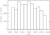 |
Fig. 1 Histogram of the number of white-light image plates available in the archive. |
In 106 years of observations, 31 800 plates covering over 31 000 days were acquired. Figure 1 shows the histogram of the number of white-light observational images. At first, only few images were acquired, but many data were collected between 1930 to 1980. The number of plates increases during the period from 1960 to 1970. This is just after the announcement of the international geophysical year (IGY). On average, about 290 white-light images were acquired each year.
3. Digitizer unit
The digitizer unit has a uniform source sphere of 1-m diameter with a front mouth opening of about 35 cm. At 3 − 4 places a halogen bulb was kept and normally one or two bulbs were alight at a time. The intensity of the light source is controlled by a constant current source. With this setup the sphere provides a highly uniform light over the opening of the sphere. Above the opening mouth of the sphere a slider is kept that can carry the photographic plate. This moves in the horizontal direction in and out of the sphere’s mouth. The photographic plates were put on the slider whenever the digitization of the plates was carried out. A CCD camera was kept in the vertical slider. The vertical slider helps in adjusting the size of the final image and also helps in focusing with fine adjustments. An imaging lens with negligible vignetting and aberrations was kept in front of the CCD camera. A green color broad-band filter was also kept in-front of the CCD to reduce the intensity and heat load on the CCD camera. A scientific grade CCD camera with a 4k × 4k format and 16 bit readout at a rate of 0.5 MHz provided by Andor technologies. A 15 μm pixel makes a 62 mm size CCD array. A 16 bit camera with a four port read-out at a rate of 500 kHz provides images with high photometric accuracies and a wide dynamic range. The CCD is cryogenic-cooled and operates at a temperature of − 100 °C. With this temperature the CCD provides a low dark current and low readout noise. Two digitizer units with the same setup were used for digitizing the white-light images.
4. Digitization of white-light images
The photographic plates are illuminated with uniform light source coming from the sphere. The images of the photographic plates were taken with an exposure time of 5 − 30 s depending on the transparency of the plates. The higher the transparency, the shorter the time of exposure, and vice versa. While digitizing the data sets, the dark current was subtracted from each image. The flats were taken by placing a clean glass plate on the horizontal slider, which is of the same thickness as the photographic plates. Before starting each month’s data digitization, two to three flats were taken. The same setup and procedure was followed for all data sets. Data were stored on the hard disk of the computer at Kodaikanal observatory and a copy was kept at the Data Center of the Indian Institute of Astrophysics, Bengaluru. Thumbnail images of all raw and calibrated data are available through the website http://kso.iiap.res.in. Daily images are available through a search engine developed in-house at IIA using Java and Mysql database. The website shows raw and calibrated jpeg images starting from 1904 until today. The final data products along with full-resolution FITS images will be made available for the scientific community through this web portal in the near future.
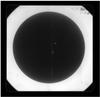 |
Fig. 2 Digitized white-light image of the full disk of the Sun. The image was digitized with 4096 × 4096 pixels resulting in a plate scale of 0.62 arcsec per pixel. The central white line represents the east-west line on the sky. The date and time of the observations are shown in the top right corner of the image. The image was obtained on March 27, 1938 at 08:10 h. |
Figure 2 shows a representative example of the digitized white-light image. The image is a photographic negative. A bright vertical line in the center of the image indicates the location of the east-west direction in the sky. The date and time of the observations are written in one corner of the image. Beyond the solar disk the unexposed part of the plate is white and can be used for stray-light estimation. Sometimes there are scratches and dust/fungus on the plates. The dust that is located on the reverse side of the emulation was removed with a clean cloth. However, there still remain some dust particles on the emulation side.
5. Data calibration
Before using the digitized data for scientific analysis, it is essential to calibrate the data. This includes the flat-fielding of the digitized data, centering the solar disk with the image window, orient the north polarity upward and correct for the photographic density values. We describe each of these in the next subsections.
5.1. Flat-fielding of the digitized data
For each month of data digitization, two to three flat-field images were recorded and saved. These flat images are dark-subtracted. The average flat -field was constructed and later used to correct the CCD pixel-to-pixel gain variations. This was done for all images at their original resolution.
5.2. Locating the solar disk center and radius
We locate the solar disk center and radius in terms of pixels or arc seconds. Many different methods have been adopted in the past (Denker et al. 1999). We used a circle Hough transform to locate the solar disk center and radius (Ballard 1981). First we reduced the data to one fourth of the original size. We then used a Sobel filter to isolate the sharp edges in the solar images. This procedure not only detects the solar limb, it also detects the borders of the features and sharp gradients. To separate the solar limb from the rest of the features we used an intensity threshold of five times the mean value of the intensity of the Sobel-filtered solar disk. This procedure clearly isolates the solar limb from the rest of the features. To use the circle Hough transform it is essential to feed the approximate radius of the intended image. We first fed the approximate radius of the reduced-size image to the circle Hough transform procedure. This procedure provides the center and radius of the solar disk. Four times the value of this has been fed again into the circle Hough transform procedure to locate the center and radius of the original solar white-light image. The limb co-ordinates of the original size Sobel-filtered image was introduced to search for the center and radius of the original image. The circle Hough transform provides the center and radius of the solar disk with high accuracy.
5.3. Conversion to relative plate density
In the exposed and developed photographic plates, the blackening corresponds to the incident flux on the plates. The blackening also depends on the exposure time of the plate to the incident flux. The blackened area corresponds to the optical density of the exposed layer. This also suggests which part of the plate is absorbed a light intensity. The photographic plate density is related to the logarithm of the plate exposure through the product of the incident light intensity and exposure time. From the relation one can convert the plate density into the solar intensity values. However, there are two difficulties for incorporating this procedure into the calibration of the white-light images. The first one is that the density curves are available in the plates only after 1969. The second is that the density curve changes from day to day. To overcome these problems we calibrated the plates to relative plate density rather than to absolute intensity values. For this we used available information in the plate with the formula (Mickaelian et al. 2007) I = (V − B) / (Ti − B), where I is the relative plate density of the calibrated image in arbitrary units, V is the average pixel value for the unexposed part of the plate, B is the average value of the darkest pixel and Ti is the density value at each pixel location. This procedure is similar to the one adopted by Ermolli et al. (2009) to calibrate the Ca II K images obtained from various observatories around the world.
5.4. Image-centering and rotation
Most of the time the solar disk in the photographic plate is not in the center of the image window. From the procedure adopted in Sect. 5.2, we have the information about the center and radius of the solar disk in the image window. With this information we shifted the solar disk so that the center of the image window and the center of the solar circle match. Later, we automatically detected the east-west line in the original image that goes from bottom to top in the image. This was made by selecting the large rectangular sized window in the center of the image and using a threshold value to detect the line automatically. We then computed the angle made by this line with respect to the vertical line. We then computed a P-angle for the epoch and added the P-angle to the east-west angle and then rotated the image by this angle. This procedure oriented the images in such away that the northpole of the image is always directed upward. Later, we examined each and every image for the north polarity direction to make sure that it was performed uniformly in all images.
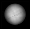 |
Fig. 3 Calibrated and aligned white-light image. The full image size is 4096 × 4096 pixels. Each pixel corresponds to 0.62 arcsec. The image was obtained on March 27, 1938 at 08:10 h. |
Figure 3 shows the processed image sample of calibrated and aligned white-light image. Clearly, the sunspots are aligned in the east-west direction. In many of the images the boundary between the umbra and penumbra can be clearly demarcated. Even the limb has a sharp boundary in the image. Apart from these there is some dirt in the image that is seen as white or black spots depending on whether it is dirt or a scratch on the image. The dark line is the east-west line on the sky.
5.5. Corrected image and image header
In the final stage of the calibration procedure we saved the corrected images (which includes all procedures mentioned above) in the FITS format with relevant information in the header. This includes the date and time of the photographic plate, the center and radius of the solar disk in the image, and the approximate pixel resolution of the image.
We calibrated the white-light data starting from 1920 to 2011, which covers a period of about 92 years. But 15 years of data still have to be calibrated. In this period, about four years of data have a different spatial resolution. The solar image is much larger than the images available after 1920. The images taken from 1905 to 1909 have north-south and east-west cross lines. In the second stage of calibration we discuss these issues.
6. Properties of white-light image time series
The 106 years of white-light data sets are not uniform throughout the time series. Each day image is different from the next in contrast. This is because the seeing is different on different days of the observations and sometimes passing clouds were present when the images were taken. Moreover, the image acquisition has changed from photographic plates to films in the later part of the twentieth century. Although the optics was not changed over 90 years, there could be degradation in the quality. There could be an increased scattered light in the images. This eventually degrades the quality of the images. Some of the properties of long time series of the data sets are compared below. Some of these procedures are similar to those followed by Ermolli et al. (2009).
6.1. Image contrast
The contrast of the image is a quantity that provides information about the quality of the image. The images are not intensity-calibrated, which requires the plate γ parameter, which depends on the plate emulsion and the plate development process (de Vaucouleurs 1968). The plate γ parameter is an indicator of the image contrast. Naturally, the image contrast measured over many years indicates how the plate γ parameter changed over the years. We measured the variation in the relative plate density over the solar disk from center to limb. This was made by constructing 25 rings of equal area from center to limb. At each ring we obtained a median value. From the set of median values we obtained the minimum and maximum values. We then computed the contrast of the image by taking the ratio of the difference and sum of the maximum and minimum values.
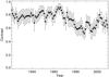 |
Fig. 4 Yearly averaged image contrast as a function of time. The vertical bars represent the root mean square value of the contrast computed over the year of white-light data. |
Figure 4 shows a plot of the mean value of the image contrast over the 90 years of data. The contrast values were obtained by averaging the data values over the years. The image contrast was varying from 0.8 − 0.9 starting from 1920 to 1970. However, there is a decline in the image contrast from 1970 onward until the recent past. This could be due to various reasons. The optics were possibly old and were maybe not cleaned over the time. The photographic plates have changed to films during this period. It could also be due to the seeing, which has changed over the time. By looking at the data over all the years there is a definite change in the image clarity from 1920 to 2011. The vertical bars represent the rms value of the contrast over the year.
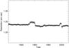 |
Fig. 5 Yearly averaged spatial resolution of the white-light image as a function of time. The vertical bars show the root mean square value over the data points. In many cases it is lower than the width of the data points. |
6.2. Spatial resolution
The spatial resolution of the image provides an idea about the spatial information in the images. The central 128 × 128 box was used for estimating the spatial resolution of the white-light images. A power spectral analysis was adopted to compute this parameter. A majority of the information about the features observed in the images lies in the low-frequency range. The frequency at which 98% of the total power spectral density remains is taken as the spatial resolution of the images. Figure 5 shows the variations of the spatial resolution over a period of 90 years. The yearly average of spatial resolution is plotted here. The vertical bar represents the rms value. The rms values are very low, they have the same size as the width of the symbol used in the plot. During the period from 1956 to 1960 the spatial resolution is lower than rest of the data points. However, the difference is very small. From the plot it is clear that the spatial resolution is almost constant over time with small variations.
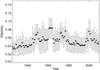 |
Fig. 6 Temporal variations of the image shape. The data points are obtained from yearly averaged values. |
6.3. Ellipticity of the image
Most of the images taken earlier in certain wavelengths are not perfectly circular in shape. This is true for the images made using the scanning spectrometer. However, the direct images taken from the telescope are not distorted. They appear almost circular in shape unless the photographic plates were kept oblique to the image. To determine the ellipticity in the white-light images we first detected the limb in the original image with the Sobel filter. The ellipse-fitting procedure provided the length of the two axes. Then the eccentricity was computed as  , where rmajor and rminor are the length of the major and minor axes. The ellipticity was computed for 90 years of data.
Figure 6 shows a plot of the ellipticity variation in the image over time. Each point shows the yearly eccentricity average and the vertical bar is the rms value computed over the year. The plot shows that there is a slight variation in the ellipticity, which could be due to the quality of the image, or to a slight variation in fitting the elliptical to the detected limb points. The ellipticity value is also very low and is close to the ellipticity value of the recent data taken with the CCD cameras (Ermolli et al. 2009). We would like to point out here that we did not measure the ellipticity that can arise from the atmospheric refraction. Previously, Sivaraman et al. (1993) corrected for the atmospheric refraction in the limb and for the individual sunspot umbral area. In a subsequent study, we are planning to examine the effects of atmospheric refraction on the geometry of the image.
7. Sunspot area coverage
In white-light images the sunspots are the prominent structures visible on the solar disk. However, near the limb side faculaes are visible as well. The sunspot number and the area coverage vary over the solar cycle and also from cycle to cycle. A strong solar activity is visible on the sun whenever many sunspots with larger area coverage appear on the solar disk. On the other hand, the solar activity reaches minimum when there are fewer sunspots. Though the sunspot areas were analyzed in the past with various data sets, it would be interesting to examine the sunspot areas obtained from the Kodaikanal white-light images with modern techniques of feature detection.
To identify the sunspots in white-light calibrated images we used a modified version of the sunspot tracking and recognition algorithm (STARA, Watson et al. 2009). First, we reduced the size of the data from 4k × 4k to 1k × 1k. Then the image was inverted in such a way that the sunspots appear as bright as shown in Fig. 7. Following Watson et al. (2009), we used a top-hat transform on the inverted Kodaikanal white-light images. The top-hat transform is an original image that is subtracted from the image, which is modified by the opening operation. This procedure makes the background flat and the sunspots appear as peaks. More details on this algorithm can be found in Watson et al. (2009). A slight difference between their method and ours is that we applied this procedure twice to the digitized white-light images with different intensity thresholds. In both cases we used same structuring element with a circle of diameter of 16 pixels. In the first step it detects all sunspots that appear near the limb and close to the limb. In the second run it identifies all sunspots that appear inside the solar disk up to μ = 0.2. Although the sunspot detection is automatic, the procedure not only detects the sunspots, it also detects the dirt and the east-west line in the sky. To remove all these additional features we added contours on the detected features and then used a cursor to identify the contours that belong to the sunspot. Despite this is slight human intervention, this provides the best results in discarding the redundant features on the photographic plates.
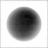 |
Fig. 7 Inverted image used for detecting the sunspots. The image size is 1024 × 1024 pixels, each pixel corresponds to 2.5 arcsec. The sunspots are visible in the full-disk image as white spots. The image was obtained on January 08, 1938 at 08:18 h. |
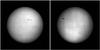 |
Fig. 8 Sunspots with the contours overlaid upon the image. Left and right side panels correspond to images recorded on Jan. 08 and Jan. 15, 1938. The image size is 1024 × 1024 pixels and each pixel corresponds to 2.5 arcsec. |
Figure 7 shows the inverted calibrated image. There are several sunspot groups visible on the disk. Some of the spots are huge and others are small. Figure 8 (left panel) shows the sunspots with the contours. Here the sunspot group is small and the algorithm detects all small sunspot groups. Figure 8 (right panel) shows another example. The large sunspot group is detected by the algorithm. The area of the detected sunspot group is corrected for the area foreshortening, then the sunspot area is converted into the millionth of a hemisphere on the Sun. Finally, we summed the entire sunspot area that appeared on the Sun on that day and stored it in a file where the first column indicates the date of the observation and the second column indicates the sunspot area. This method of estimating the sunspot area does not distinguish between the northern and southern hemisphere.
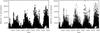 |
Fig. 9 Left: daily sunspot area computed using the Kodaikanal white-light data as a function of time. Right: same as the left-side plot but for Greenwich data. |
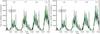 |
Fig. 10 Left: monthly averaged sunspot area data obtained from Kodaikanal and Greenwich are overplotted on each other. Right: same as the left-side plot but for the monthly median. |
A modified version of STARA was applied to the calibrated white-light data to detect the sunspots, i.e., from 1921 to 1960 spanning about 40 years. The data set includes four solar cycles. Figure 9 (left panel) shows a plot of the daily sunspot area shown over 40 years. The plot clearly shows the solar cycle variation of sunspot area. During the maximum, the sunspot area coverage over the solar disk exceeds an 8000 millionth of hemisphere (μH). However, the area coverage varies for different solar cycles. In solar cycle 16 the area coverage is small. On the other hand, cycle 19 has a large area coverage compared to cycle 16. We also compared our sunspot area results with the Greenwich sunspot area compiled by David Hathaway (http://solarscience.msfc.nasa.gov/greenwch.shtml). Figure 9 (right panel) shows the plot of the Greenwich sunspot area for the same period. Comparison of this plot with Fig. 9 (left panel) shows the similarity between the two except for the maximum area coverage during the sunspot maximum. Otherwise the pattern of the area coverage is almost the same, which suggests the goodness of the data and method of identifying the sunspots and groups.
Figure 10 (left panel) shows a monthly average of the Kodaikanal sunspot area (thick dark line) and the monthly average of the Greenwich sunspot area (dashed line with green color). The plot shows that the two monthly averaged sunspot areas match very well with a correlation coefficient of 0.97. Most of the time the Kodaikanal monthly average is little higher than the Greenwich monthly averaged sunspot area. However, the opposite is also true. We also plotted the monthly median of the sunspot area calculated from both data sets (Fig. 10 (right)). Here we see a similar correlation between the two data sets.
We then compared the yearly averaged sunspot area of the Kodaikanal and Greenwich data (Fig. 11). Although it appears that the pattern is almost the same, there are certain differences between them. In some cases the year of the sunspot maximum is different. At other times there is a double peak in the Kodaikanal data that is absent from Greenwich data. Figure 12 shows the scatter plot of the yearly averaged sunspot area of the Kodaikanal and Greenwich data sets. The obtained correlation coefficient is 0.99. The scatter is very small in the smaller area and it is larger for the larger area.
In Fig. 13 we compare the monthly averaged Kodaikanal sunspot area with the monthly averaged Greenwich sunspot number. The comparison shows that the correlation between the sunspot number and the sunspot area is good. However, there are certain differences between them. For example, in cycle 17 during the rising phase of the sunspot number there is a sharp rise in the sunspot area, but the increase in sunspot number is marginal. These differences can be found in many places. On the other hand, although there is an increase in sunspot number in cycle 19 during the peak time, the sunspot area decreased, meaning there could be many small sunspots whose total area will be small. This kind of anti-correlation between sunspot number and area can be found in many cycles. It suggests that there could be a large sunspot with larger apparent area although the number of sunspots on the Sun could be small. This can be clearly seen in the scatter plot of the monthly averaged Greenwich sunspot numbers and the monthly averaged Kodaikanal sunspot area (Fig. 14). In the plot at some places there are few spots, but the area is large.
8. Conclusions
In Kodaikanal, white-light observations of the Sun on photographic plates and films have been made since 1904. The white-light images have been collected for more than 105 years with 290 images on average per year. These data sets were recently digitized at Kodaikanal and about 90 years of data were calibrated and aligned. They have a uniform spatial resolution. This is mainly because the same optics were used throughout the 90 years, starting from 1920 until today. Before 1920 there were some changes to the optics and hence the obtained images are slightly larger. The contrast of the images is quite good until 1970, after which it started to decrease slightly. This is the period where the observations changed from photographic plate to films. In the linear part of the characteristic curve, the density parameter of the plate is proportional to the logarithm of the exposure parameter with the γ function as a slope. The γ parameter depends on the emulsion of the photographic plates and also on how the plates were developed. In a way the γ parameter represents the image contrast. The image contrast declined after 1970, suggesting that there is a change in the γ parameter, which likely implies a change in the plate emulation composition. This also indicates that for a detailed quantitative analysis one needs to use the γ parameter for intensity calibration purposes. We intend to do this in the future. But for the current study of the sunspot area this may not be required. The image shape is almost circular and does not show any oblateness. We performed a relative calibration to the digitized images by using the information available on the plates. We also corrected for the image orientation and centering. However, we did not yet correct for the scattered light, which we plan for the next step.
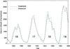 |
Fig. 11 Yearly averaged sunspot area data obtained from Kodaikanal and Greenwich overplotted. |
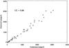 |
Fig. 12 Scatter plot of the Kodaikanal and Greenwich sunspot area. |
Sunspot area measurements over a long time period are valuable and important data for studying the solar activity on the Sun. The solar activity is responsible for the variations in EUV and X-ray radiation emitted from the Sun. The changes in the Earth’s upper atmosphere are modulated by the observed solar activity (She et al. 2002). The digitized Kodaikanal white-light images could be complimentary data for studying the variations in sunspot and faculae areas over 100 years that may have influenced changes in the Earth’s upper atmosphere. By using a semi-automated code to detect the features on the Sun we identified and detected all sunspots visible on the Sun. We measured sunspot area and groups of sunspots on each day. A correction for the projection effect was also included. While the measured area is well-correlated with the Greenwich sunspot area, the area measured by the Kodaikanal white-light data is slightly larger than that of Greenwich. There is a high correlation of monthly mean and median values of the sunspot area of the Kodaikanal and Greenwich data. However, there is a slight offset between the peak times of the sunspot maximum in a few cycles when we looked at the yearly averaged sunspot area of Kodaikanal and Greenwich. The yearly averaged sunspot area of Kodaikanal and Greenwich is very highly correlated at 0.99. Even the monthly averaged sunspot number obtained from Greenwich follows the pattern of monthly averaged Kodaikanal sunspot areas very closely. The scatter plot of the two shows a correlation coefficient of about 0.91. This high degree of correlation of the Kodaikanal sunspot area with that of Greenwich suggests that one can also accurately extract the information about the features with the Kodaikanal data. Hence, the sunspot area obtained from the Kodaikanal observatory white-light images can be directly used to estimate solar irradiance variations with a minimal intercalibration with other data sets (Balmaceda et al. 2009).
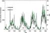 |
Fig. 13 Monthly averaged sunspot area obtained from Kodaikanal and the sunspot number obtained from Greenwich for four solar cycles. |
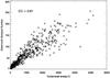 |
Fig. 14 Scatter plot of the monthly averaged sunspot area and sunspot number. |
Kodaikanal has been taking white-light, Ca K, and Hα data for the past 100 years. Although many observatories have made similar kinds of observations in the past and in recent times, the Kodiakanal data are uniform over the past 100 years. The optics and processing of the plates were kept uniform. However, the photographic plate has been replaced with films and at the same time there is a reduction in the contrast of the images. Hence, to keep the quality of the data uniform, it is essential to calibrate the images to intensity format. But for the current study of sunspot area calculations it is not required to intercalibrate the data. This is an advantage in studying the solar irradiance etc. (see also Ermolli et al. 2009). A few more years of data need to be calibrated, which will be taken up soon. In the future, we aim to compare the results of extracted parameters using different techniques with the other data sets available all around the world. Our impression is that sunspot areas may turn out to be a better proxy than sunspot numbers for studying the magnetic activity variation, particularly on shorter time scales.
Acknowledgments
We would like to thank many observers at Kodaikanal, who have observed the Sun in white-light and made it available to us. Special thanks go to Jagdev Singh, who has initiated this new digitization program several years ago. We thank Rekhesh Mohan, N. Sneha, Nimesh Sinha, Ayeha Banu, S. Kamesh, P. Manikantan, and Janani for their help at different phases. We also would like to thank the staff members at Kodaikanal, who helped us in setting up the digitizer unit and carry out the digitization at Kodaikanal. Finally we would like to thank the referee, R. Ulrich, for his valuable comments and suggestions, which improved the quality of the presentation.
References
- Ballard, D. H. 1981, Pattern Recognition, 13, 111 [CrossRef] [Google Scholar]
- Balmaceda, L. A.,Solanki, S. K.,Krivova, N. A., &Foster, S. 2009, J. Geophys. Res. (Space Physics), 114, 7104 [Google Scholar]
- Bappu, M. K. V. 1967, Sol. Phys., 1, 151 [NASA ADS] [CrossRef] [Google Scholar]
- Baumann, I., &Solanki, S. K. 2005, A&A, 443, 1061 [NASA ADS] [CrossRef] [EDP Sciences] [Google Scholar]
- Denker, C.,Johannesson, A.,Marquette, W., et al. 1999, Sol. Phys., 184, 87 [NASA ADS] [CrossRef] [Google Scholar]
- de Vaucouleurs, G. 1968, Appl. Opt., 7, 1513 [Google Scholar]
- Ermolli, I.,Solanki, S. K.,Tlatov, A. G., et al. 2009, ApJ, 698, 1000 [NASA ADS] [CrossRef] [Google Scholar]
- Hasan, S. S., Mallik, D. C. V., Bagare, S. P., & Rajaguru, S. P. 2010, in Magnetic Coupling between the Interior and Atmosphere of the Sun, eds. S. S. Hasan, & R. J. Rutten, 12 [Google Scholar]
- Mickaelian, A. M.,Nesci, R.,Rossi, C., et al. 2007, A&A, 464, 1177 [NASA ADS] [CrossRef] [EDP Sciences] [Google Scholar]
- She, C. Y.,Sherman, J.,Vance, J. D., et al. 2002, J. Atmos. Sol. Terr. Phys., 64, 1651 [NASA ADS] [CrossRef] [Google Scholar]
- Sivaraman, K. R.,Gupta, S. S., &Howard, R. F. 1993, Sol. Phys., 146, 27 [NASA ADS] [CrossRef] [Google Scholar]
- Smith, C. M. 1895, PASP, 7, 113 [NASA ADS] [CrossRef] [Google Scholar]
- Watson, F.,Fletcher, L.,Dalla, S., &Marshall, S. 2009, Sol. Phys., 260, 5 [NASA ADS] [CrossRef] [Google Scholar]
All Figures
|
Fig. 1 Histogram of the number of white-light image plates available in the archive. |
| In the text | |
|
Fig. 2 Digitized white-light image of the full disk of the Sun. The image was digitized with 4096 × 4096 pixels resulting in a plate scale of 0.62 arcsec per pixel. The central white line represents the east-west line on the sky. The date and time of the observations are shown in the top right corner of the image. The image was obtained on March 27, 1938 at 08:10 h. |
| In the text | |
|
Fig. 3 Calibrated and aligned white-light image. The full image size is 4096 × 4096 pixels. Each pixel corresponds to 0.62 arcsec. The image was obtained on March 27, 1938 at 08:10 h. |
| In the text | |
|
Fig. 4 Yearly averaged image contrast as a function of time. The vertical bars represent the root mean square value of the contrast computed over the year of white-light data. |
| In the text | |
|
Fig. 5 Yearly averaged spatial resolution of the white-light image as a function of time. The vertical bars show the root mean square value over the data points. In many cases it is lower than the width of the data points. |
| In the text | |
|
Fig. 6 Temporal variations of the image shape. The data points are obtained from yearly averaged values. |
| In the text | |
|
Fig. 7 Inverted image used for detecting the sunspots. The image size is 1024 × 1024 pixels, each pixel corresponds to 2.5 arcsec. The sunspots are visible in the full-disk image as white spots. The image was obtained on January 08, 1938 at 08:18 h. |
| In the text | |
|
Fig. 8 Sunspots with the contours overlaid upon the image. Left and right side panels correspond to images recorded on Jan. 08 and Jan. 15, 1938. The image size is 1024 × 1024 pixels and each pixel corresponds to 2.5 arcsec. |
| In the text | |
|
Fig. 9 Left: daily sunspot area computed using the Kodaikanal white-light data as a function of time. Right: same as the left-side plot but for Greenwich data. |
| In the text | |
|
Fig. 10 Left: monthly averaged sunspot area data obtained from Kodaikanal and Greenwich are overplotted on each other. Right: same as the left-side plot but for the monthly median. |
| In the text | |
|
Fig. 11 Yearly averaged sunspot area data obtained from Kodaikanal and Greenwich overplotted. |
| In the text | |
|
Fig. 12 Scatter plot of the Kodaikanal and Greenwich sunspot area. |
| In the text | |
|
Fig. 13 Monthly averaged sunspot area obtained from Kodaikanal and the sunspot number obtained from Greenwich for four solar cycles. |
| In the text | |
|
Fig. 14 Scatter plot of the monthly averaged sunspot area and sunspot number. |
| In the text | |
Current usage metrics show cumulative count of Article Views (full-text article views including HTML views, PDF and ePub downloads, according to the available data) and Abstracts Views on Vision4Press platform.
Data correspond to usage on the plateform after 2015. The current usage metrics is available 48-96 hours after online publication and is updated daily on week days.
Initial download of the metrics may take a while.