| Issue |
A&A
Volume 550, February 2013
|
|
|---|---|---|
| Article Number | A74 | |
| Number of page(s) | 14 | |
| Section | Numerical methods and codes | |
| DOI | https://doi.org/10.1051/0004-6361/201220126 | |
| Published online | 29 January 2013 | |
FitSKIRT: genetic algorithms to automatically fit dusty galaxies with a Monte Carlo radiative transfer code
Sterrenkundig Observatorium, Universiteit Gent, Krijgslaan 281-S9, 9000 Gent, Belgium
e-mail: This email address is being protected from spambots. You need JavaScript enabled to view it.
Received: 30 July 2012
Accepted: 30 November 2012
Abstract
We present FitSKIRT, a method to efficiently fit radiative transfer models to UV/optical images of dusty galaxies. These images have the advantage that they have better spatial resolution compared to FIR/submm data. FitSKIRT uses the GAlib genetic algorithm library to optimize the output of the SKIRT Monte Carlo radiative transfer code. Genetic algorithms prove to be a valuable tool in handling the multi- dimensional search space as well as the noise induced by the random nature of the Monte Carlo radiative transfer code. FitSKIRT is tested on artificial images of a simulated edge-on spiral galaxy, where we gradually increase the number of fitted parameters. We find that we can recover all model parameters, even if all 11 model parameters are left unconstrained. Finally, we apply the FitSKIRT code to a V-band image of the edge-on spiral galaxy NGC 4013. This galaxy has been modeled previously by other authors using different combinations of radiative transfer codes and optimization methods. Given the different models and techniques and the complexity and degeneracies in the parameter space, we find reasonable agreement between the different models. We conclude that the FitSKIRT method allows comparison between different models and geometries in a quantitative manner and minimizes the need of human intervention and biasing. The high level of automation makes it an ideal tool to use on larger sets of observed data.
Key words: radiative transfer / dust, extinction / galaxies: structure / galaxies: individual: NGC 4013
© ESO, 2013
1. Introduction
In the past few years, the importance of the interstellar dust medium in galaxies has been widely recognized. Dust regulates the physics and chemistry of the interstellar medium, and reprocesses about one third of all stellar emission to infrared and submm emission. Nevertheless, the amount, spatial distribution and physical properties of the dust grains in galaxies are hard to nail down.
The most direct method to trace the dust grains in galaxies is to measure the thermal emission of the dust grains at mid-infrared (MIR), far-infrared (FIR) and submm wavelengths. Obtaining total dust masses from MIR, FIR or submm images should in principle be straightforward, as dust emission is typically optically thin at these wavelengths and thus total dust masses can directly be estimated from the observed spectral energy distribution. There are a number of problems with this approach, however. One complication is the notoriously uncertain value of the dust emissivity at long wavelengths (Bianchi et al. 2003; Kramer et al. 2003; Alton et al. 2004; Shirley et al. 2011) and the mysterious anti-correlation between the dust emissivity index and dust temperature (Dupac et al. 2003; Shetty et al. 2009; Veneziani et al. 2010; Juvela & Ysard 2012b,a; Kelly et al. 2012; Smith et al. 2012a). A second problem is the difficulty to observe in the FIR/submm window, which necessarily needs to be done from space using cryogenically cooled instruments. Until recently, the available FIR instrumentation was characterized by limited sensitivity and wavelength coverage, and the submm window was largely unexplored. This has now partly changed thanks to the launch of the Herschel (Pilbratt et al. 2010) satellite, but also this mission has a very limited lifetime. Finally, the third and most crucial limitation is the poor spatial resolution of the available FIR/submm instruments (typically tens of arcsec). This drawback is particularly important if we want to determine the detailed distribution of the dust in galaxies rather than just total dust masses. This poor spatial resolution limits a detailed study of the dust medium to the most nearby galaxies only (e.g. Meixner et al. 2010; Bendo et al. 2010, 2012; Xilouris et al. 2012; Foyle et al. 2012; De Looze et al. 2012b; Fritz et al. 2012; Smith et al. 2012a; Galametz et al. 2012). Moreover, several authors have demonstrated that even estimating total dust masses from global fluxes induces an error due to resolution effects (Galliano et al. 2011; Galametz et al. 2012).
The alternative method to determine the dust content in galaxies is to use the extinction effects of the dust grains on the stellar emission in the UV, optical or near-infrared (NIR) window. This wavelength range has the obvious advantages that observations are very easy and cheap, and that the spatial resolution is an order of magnitude better than in the FIR/submm window. Furthermore, the optical properties of the dust are much better determined in the optical than at FIR/submm wavelengths. The main problem in using this approach is the difficulty to translate attenuation measurements from broadband colors to actual dust masses, mainly because of the complex and often counter-intuitive effects of the star/dust geometry and multiple scattering (Disney et al. 1989; Witt et al. 1992; Byun et al. 1994; di Bartolomeo et al. 1995; Baes & Dejonghe 2001b; Inoue 2005). Simple recipes that directly link an attenuation to a dust mass are clearly not sufficient; the only way to proceed is to perform detailed radiative transfer calculations that do take into account the necessary physical ingredients (absorption, multiple anisotropic scattering) and that can accommodate realistic geometries. Fortunately, several powerful 3D radiative transfer codes with these characteristics have recently been developed (e.g. Gordon et al. 2001; Baes et al. 2003, 2011; Jonsson 2006; Bianchi 2008; Robitaille 2011).
A state-of-the-art radiative transfer code on itself, however, is not sufficient to determine the dust content of galaxies from UV/optical/NIR images. A radiative transfer simulation typically starts from a 3D distribution of the stars and the dust in a galaxy model and calculates how this particular system would look for an external observer at an arbitrary viewing point, i.e. it simulates the observations. The inverted problem, determining the 3D distribution of stars and dust from a given reference frame, is a much harder nut to crack. It requires the combination of a radiative transfer code and an optimization procedure to constrain the input parameters. Several fitting codes that combine a radiative transfer code with an optimization algorithm have been set up (Xilouris et al. 1997; Steinacker et al. 2005; Robitaille et al. 2007; Bianchi 2007; Schechtman-Rook et al. 2012). All too often, however, this optimization procedure is neglected and chi-by-eye models are presented as reasonable alternatives.
To optimize this given problem it is important to realize that the parameter space is quite large, easily going up to 10 free parameters or more. As discussed before, the complexity of the dust/star geometry and scattering off dust particles is often counter-intuitive and results in a non-linear, non-differentiable search space with multiple local extrema. Furthermore, there is another inconvenient feature induced by the radiative transfer code. Most state-of-the-art radiative transfer codes are Monte Carlo codes where the images are constructed by detecting a number of predefined photon packages. Because of the intrinsic randomness of the Monte Carlo code, images always contain a certain level of Poisson noise. If one runs a forward Monte Carlo radiative simulation, it is usually straightforward to make the number of photon packages in the simulation so large that this noise becomes negligibly small. However, if we want to couple the radiative transfer simulation to an optimization routine, typically many thousands of individual simulations need to be performed, which inhibits excessively long run times for each simulation and hence implies that there will always be some noise present. As a result, we have to fit noisy models to noisy data, as reduced CCD data will always contain a certain level of noise (Newberry 1991).
For complex optimization problems like this, it is not recommended to use classical optimization methods like the downhill simplex or Levenberg-Marquardt methods, but rather apply a stochastic optimization method instead. The main advantage of stochastic methods such as simulated annealing, random search, neural networks, and genetic algorithms over most classical optimization methods is their ability to leave local extrema and search over broad parameter spaces (Fletcher et al. 2003; Theis & Kohle 2001; Rajpaul 2012b). Genetic algorithms (Goldberg 1989; Mitchell 1998) are one class of the stochastic optimization methods that stands out when it comes to noisy handling because it works on a set of solutions rather than iteratively progressing from one point to another. Genetic algorithms are often applied to optimize noisy objective functions (Metcalfe et al. 2000; Larsen & Humphreys 2003). During the past decade, genetic algorithms have become increasingly more popular in numerous applications in astronomy and astrophysics ranging from cosmology and gravitational lens modeling to stellar structure and spectral fitting (Charbonneau 1995; Metcalfe et al. 2000; Theis & Kohle 2001; Larsen & Humphreys 2003; Fletcher et al. 2003; Liesenborgs et al. 2006; Baier et al. 2010; Schechtman-Rook et al. 2012; Rajpaul 2012a). For a recent overview of the use of genetic algorithms in astronomy and astrophysics, see Rajpaul (2012b).
In this paper, we present FitSKIRT, a tool designed to efficiently model the stellar and dust distribution in dusty galaxies by fitting radiative transfer models to UV/optical/NIR images. The optimization routine behind the FitSKIRT code is based on genetic algorithms, which implies that the code is able to efficiently explore large, complex parameter spaces and conveniently handle the noise induced by the radiative transfer code. Bias by human intervention is kept to an absolute minimum and the results are determined in an objective manner. In Sect. 2 the radiative transfer code and the genetic algorithm are discussed in more detail. We also apply the genetic algorithms library on a complex but analytically tractable optimization problem to check its reliability and efficiency. This knowledge is then used to explain the major steps and features of the FitSKIRT program. In Sect. 3 we test the FitSKIRT program on reference images of which the input values are exactly known. This should allow us to have a closer look at the complexity of the problem and FitSKIRTs ability to obtain reasonable solutions in an objective way. In Sect. 4 we apply FitSKIRT to determine the intrinsic distribution of stars and dust in the galaxy NGC 4013, and we compare the resulting model to similar models obtained by Bianchi (2007) and Xilouris et al. (1999). Section 5 sums up.
2. FitSKIRT
2.1. The SKIRT radiative transfer code
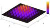 |
Fig. 1 The function defined by Eq. (1) for n = 9. It contains many steep local maxima surrounding the global maximum at (x,y) = (0.5,0.5) and is therefore a strong test function for global optimization algorithms. |
SKIRT (Baes et al. 2011) is a 3D continuum Monte Carlo radiative transfer code, initially developed to investigate the effects of dust absorption and scattering on the observed gas and stellar kinematics of dusty galaxies (Baes & Dejonghe 2002; Baes et al. 2003). The code has continuously been adapted and upgraded to a general and multi-purpose dust radiative transfer code. It now includes many advanced techniques to increase the efficiency, including forced scattering (Mattila 1970; Witt 1977), the peeling-off technique (Yusef-Zadeh et al. 1984), continuous absorption (Lucy 1999), smart detectors (Baes 2008) and frequency distribution adjustment (Bjorkman & Wood 2001; Baes et al. 2005). The code is capable of producing simulated images, spectral energy distributions, temperature maps and observed kinematics for arbitrary 3D dusty systems. SKIRT is completely written in C++ in an object-oriented programming fashion so it is effortless and straightforward to implement and use different stellar or dust geometries, dust mixtures, dust grids, etc.
The default mode in which SKIRT operates is the panchromatic mode. In this mode, the simulation covers the entire wavelength regime from UV to millimeter wavelengths and guarantees an energy balance in the dust, i.e. at every location in the system, the emission spectrum of the dust at infrared and submm wavelengths is determined self-consistently from the amount of absorbed radiation at UV/optical/NIR wavelengths. In this mode, the SKIRT code is easily parallelized to run on shared memory machines using the OpenMP library: every single thread deals with a different wavelength. This panchromatic SKIRT code has been used to predict and interpret the far-infrared emission from a variety of objects, including edge-on spiral galaxies (Baes et al. 2010, 2011; De Looze et al. 2012b), elliptical galaxies (De Looze et al. 2010; Gomez et al. 2010), active galactic nuclei (Stalevski et al. 2011, 2012) and post-AGB stars (Vidal & Baes 2007).
Besides the panchromatic mode, it is also possible to run SKIRT in a monochromatic mode so it is less time consuming when one wants to model images at one particular wavelength. In this mode, the OpenMP parallelization is included by distributing the different photon packages in the simulation over all available threads, which implies that some precautions must be taken to avoid race conditions. This monochromatic mode is particularly useful when one wants to fit radiative transfer models to a particular observed image at UV, optical or near-infrared wavelengths, which we deal with in this paper.
2.2. The GAlib genetic algorithm library
Genetic algorithms are problem solving systems based on evolutionary principles. In essence evolution theory describes an optimization process of a population to a given environment. The core difference between genetic algorithms and most other stochastic methods is that a genetic algorithm works with a set (population) of possible solutions (individuals) to the problem (environment). Each individual consists of a number of parameters (genes). For each of these genes there is a number of possible values which we call alleles. These alleles do not have to be a discrete set, but can be defined as a range or pool where the genes should be drawn from.
The algorithm starts by defining both the size and the content of the initial population (generation 0). The individuals can be created randomly from the gene pool or they can be manually defined. Each of the initial solutions is then evaluated and given a certain “fitness” value. The individuals that meet certain criteria of fitness are then used to crossover and produce the first offspring (generation 1). Another, more convenient way of determining which individuals are fit for reproduction is by determining a crossover rate. If, for example, the crossover rate is set to 0.6, the 60% best individuals will be used to produce offspring. We can also define a mutation rate in a similar way. This rate determines what the odds are for a certain gene (and not individuals) of the offspring to undergo a random mutation. In practice this is done by removing one of the gene values and replacing it with a new possible value. After this step we return the fitness value. The individuals fit for reproduction are then selected and a new generation (generation 2) is created. This cycle is then repeated until a certain fitness value is obtained or until a pre-defined number of generations is reached. Since the better individuals of a population are always preferred, we expect the population average to shift to a better value where the better individuals are preferred again, etc.
Genetic algorithms have been applied successfully to a large range of test problems, and are nowadays widely used as a reliable class of global optimizers. They are becoming increasingly popular as a tool in various astrophysical applications. Most astrophysical applications so far have used the publicly available PIKAIA code (Charbonneau 1995), originally developed in Fortran 77 and now available in Fortran 90 and IDL as well.
We have selected the publicly available GAlib library (Wall 1996) for our purposes. One of the main reasons for choosing GAlib is that, like the SKIRT radiative transfer code, it is written in C++ and thus guarantees straightforward interfacing. Moreover, the library has been properly tested and adapted over the years and has been applied in many scientific and engineering applications. It comes with an extensive overview of how to implement a genetic algorithm and examples illustrating customizations of the GAlib classes. To illustrate the performance of the GAlib library, we have applied it to the same test function as first suggested by Charbonneau (1995) but also investigated by others (Cantó et al. 2009; Rajpaul 2012b). The goal of the exercise is the find the global maximum of the function ![Mathematical equation: \begin{equation} f(x,y) = \Bigl[ 16\,x\,(1-x)\,y\,(1-y)\sin(n\pi x)\sin(n\pi y) \Bigr]^2 \label{Charbonneau} \end{equation}](/articles/aa/full_html/2013/02/aa20126-12/aa20126-12-eq4.png) (1)in the unit square with x and y between 0 and 1. The function is plotted in Fig. 1 for n = 9. It is clear that this function is a severe challenge for most optimization techniques: the search space contains many steep local maxima surrounding the global maximum at (x,y) = (0.5,0.5). In addition, the global maximum is not significantly higher compared to the surrounding local maxima. A classical hill climbing method would most definitely get stuck in a local maximum. An iterative hill climbing method, which restarts at randomly chosen points, would also be able to solve this problem but it would normally take much longer to do so compared to a genetic algorithm.
(1)in the unit square with x and y between 0 and 1. The function is plotted in Fig. 1 for n = 9. It is clear that this function is a severe challenge for most optimization techniques: the search space contains many steep local maxima surrounding the global maximum at (x,y) = (0.5,0.5). In addition, the global maximum is not significantly higher compared to the surrounding local maxima. A classical hill climbing method would most definitely get stuck in a local maximum. An iterative hill climbing method, which restarts at randomly chosen points, would also be able to solve this problem but it would normally take much longer to do so compared to a genetic algorithm.
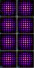 |
Fig. 2 Illustration of GAlib’s approach to find the global maximum of the function (1). The different panels show the 100 individuals of a population 0, 1, 2, 3, 4, 5, 10 and 25, characterized by a mutation probability of 0.3% and a crossover rate of 65%. For the first few generations, the individuals are distributed randomly, starting from generation 5 the individuals are clearly centered around the local maxima and continue to converge to the true maximum. |
We demonstrate how the GAlib genetic algorithm library behaves in this complex search space by plotting the contours and overplotting the position of the individuals for each generation. The results are shown in Fig. 2. For these tests we use the same values for the mutation probability and crossover rate as Charbonneau (1995), namely 0.3% and 65% respectively, and the population size is set to 100. As it is shown, the algorithm is capable of efficiently determining the maximum. Starting from generation 5 the individuals are clearly centered around the local maxima and continue to converge to the true maximum. At generation 10 all individuals are very close to the global maximum, and we note few changes between generations 10 and 25. This can be explained by the large population inertia. The large population prohibits the fast alteration to a favorable mutation. Higher mutation rates could be a possible way to increase accuracy but we have to keep in mind that this could come at the cost of losing the global maximum (Charbonneau 1995). Furthermore it is not our ultimate goal to optimize this given problem in the best possible manner.
The final result we get using this method after 25 generations is: (x,y) = (0.502,0.498) with f(x,y) = 0.994. It should be noted that this solution is not a special case and that the algorithm delivers this result almost every time. After 1000 consecutive runs we get an average result When we increase the number of generations, we obviously still recover the global maximum and reduce the standard deviation: for a population of 100 and 100 generations we get As a final example, we increase the mutation rate to 30% to show it improves the accuracy. Again after 100 generations, we now find Looking at Fig. 2 and comparing with the result, f(x,y) = 0.978322 (ranked case, 40 generations), obtained by Charbonneau (1995), it can be seen that, for this problem, GAlib performs at least as good (see the 25 generation case) as the PIKAIA code and we can be confident to use the GAlib code for our purposes1.
2.3. FitSKIRT
Our goal is to develop a fitting program that optimizes the parameters of a 3D dusty galaxy model in such a way that its apparent image on the sky fits an observed image. This comes down to an optimization function, where the objective function to be minimized is the χ2 value, ![Mathematical equation: \begin{equation} \chi^2(\boldsymbol{p}) = \sum_{j=1}^{N_{\text{pix}}} \left[\frac{I_{\text{mod},j}(\boldsymbol{p}) - I_{\text{obs},j}} {\sigma_j(\boldsymbol{p})}\right]^2 \cdot \label{chi2} \end{equation}](/articles/aa/full_html/2013/02/aa20126-12/aa20126-12-eq16.png) (2)In this expression, Npix is the total number of pixels in the image, Imod,j and Iobs,j represent the flux in the jth pixel in the simulated and observed image respectively, σj is the uncertainty, and p represents the dependency on the parameters of the 3D model galaxy. Note that, contrary to most χ2 problems, the uncertainty σj in our case depends explicitly on the model: it can be written as
(2)In this expression, Npix is the total number of pixels in the image, Imod,j and Iobs,j represent the flux in the jth pixel in the simulated and observed image respectively, σj is the uncertainty, and p represents the dependency on the parameters of the 3D model galaxy. Note that, contrary to most χ2 problems, the uncertainty σj in our case depends explicitly on the model: it can be written as 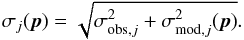 (3)The factor σobs,j represents the uncertainty on the flux in the jth pixel of the observed image, usually dominated by a combination of photon noise and read noise. It can be calculated using the so-called CCD equation (Mortara & Fowler 1981; Newberry 1991; Howell 2006). The factor σmod,j(p) represents the uncertainty on the flux in the jth pixel of the simulated image corresponding to the Monte Carlo simulation with model parameters p. It can be calculated during the Monte Carlo radiative transfer simulation according to the recipes from Gordon et al. (2001).
The full problem we now face is to minimize the χ2 measure (2) by choosing the best value of p in the model parameter space. As the link between the model image and the model parameters is non-trivial (it involves a complete radiative transfer simulation), this comes down to a multidimensional, non-linear, non-differentiable optimization problem.
 |
Fig. 3 The main flowchart of the FitSKIRT procedure. Details on the different steps are given in the text. |
Our approach to this problem resulted in the FitSKIRT program, a code that combines the radiative transfer code SKIRT and the genetic algorithm library GAlib. Figure 3 shows a flowchart of the major parts of the FitSKIRT program.
The first step in the process consists of setting up the ingredients for the genetic algorithm. This consists in the first place of defining the reference image and defining the parameterized model describing the distribution and properties of stars and dust in the model galaxy. Apart from setting up this model, we also select the range of the parameters in the model, and define all genetic algorithm parameters like crossover rate, selection and reproduction scheme, mutation rate, etc.
In the second phase the genetic algorithm loop (green flow) is started. The initial population is then created by randomly drawing the parameter values p from the predefined ranges so the genetic algorithm starts out by being uniformly spread across the entire parameter space. The next step is to evaluate which individuals provide a good fit and which do not. This is done by starting a monochromatic SKIRT simulation using the parameters p defined by the genes of the individual. Once a simulation is done we compare the resulting frame and the reference image and give the corresponding individual an objective score. Between the creation of the image and returning the actual χ2 value, the simulated frame is convolved with the point spread function (PSF) of the observed image. The third step is then concluded by returning the final χ2(p) for this individual. After the entire population has been evaluated the best models are selected and offspring is created by crossover. Depending on the mutation rate, some of the genes of these new individuals will undergo a random mutation. After this step we obtain our new generation which is about to be evaluated next. This loop continues until a predefined number of generations is reached.
Finally, when the genetic algorithm loop ends, the convolved, best fitting frame is created again and the residual frame is determined. These residual frames are useful to investigate which areas of the references frames are well fitted and which are not. They can provide additional insight on the validity and consistency of the models themselves.
In principle, the genetic algorithm searches for the best fitting model in the entire N-dimensional parameter space, where N is the number of free parameters in the model. In general, the model image, and hence the χ2 measure (2), depends in a complex, non-linear way on the different parameters in the model, such as scalelengths, viewing angles, etc. There is one exception however: the radiative transfer problem is linear with respect to the total luminosity of the system (which always is one of the parameters in the model). This allows us to treat the total luminosity separately from the other parameters, and determine its best value outside the genetic algorithm minimization routine. This step effectively decreases the dimensionality of the parameter space the genetic algorithm has to investigate from N to N − 1. In practice, this is implemented in the following way. Assume our 3D model is defined by the N parameters p = (p1,...,pN − 1,Ltot). In every step of the genetic algorithm, the code selects a set of N − 1 parameters (p1,...,pN − 1) and starts a SKIRT radiative transfer simulation to create a model image, based on these N − 1 parameters with a dummy value for Ltot, and this model image is convolved with the observed image PSF. Before the χ2 value corresponding to this set of parameters is calculated, the code determines the best fitting total luminosity of the model that minimizes the χ2 value (2) for the particular values of these N − 1 parameters. To this aim, we can use a simple one-dimensional optimization routine. Because no noise is added between the creation of the image and determining the final χ2 value of the genome and because the one-dimensional luminosity space contains no local minima, a fast and simple golden section search is able to determine the correct value easily.
Apart from finding the parameters that correspond to the model which best fits the observed image, we also want a measure of the uncertainties on these parameters. A disadvantage of most stochastic optimization methods, or more specific genetic algorithms, is that such a measure is not readily available. A way of partially solving this problem is by using a statistical resampling technique like bootstrapping or jackknifing (Press et al. 1992; Nesseris & Shafieloo 2010; Nesseris & García-Bellido 2012). This basically comes down to iteratively replacing a predefined number of the simulated points by the actual data points and comparing the resulting objective function value. Even these estimations of the standards errors should not be used heedlessly to construct confidence intervals since they remain subject to the structure of the data. Bootstrapping also requires the distribution of the errors to be equal in the data set and the regression model (Sahinler & Topuz 2007; Press et al. 1992). Since this is not entirely the case for this problem, as Eq. (2) shows, an alternative approach was used to determine the uncertainty.
Since genetic algorithms are essentially random and the parameter space is so vast and complex, the fitting procedure can be repeated multiple times without resulting in the exact same solution. The difficulty of differentiating between some individuals because of some closely correlated parameters will be reflected in the final solutions. The entire fitting procedure used here consists of running five independent FitSKIRT simulations, all with the same optimization parameters. The standard deviation on these five solutions is set as an uncertainty on the “best” solution (meaning the lowest objective function value). While computationally expensive, this method still allows for better solutions to be found. The spread gives some insight in how well the fitting procedure is able to constrain some parameters and which parameters correlate. When the solutions are not at all coherent, this can also indicate something went wrong during the optimization process (i.e. not enough individuals or evaluated generations).
3. Application on test images
In this section, we apply the FitSKIRT code on a simulated test image, in order to check the accuracy and effectiveness of this method in deriving the actual input parameters.
3.1. The model
The test model consists of a simple but realistic model for a dusty edge-on spiral galaxy, similar to the models that have been used to actually model observed edge-on spiral galaxies (e.g. Kylafis & Bahcall 1987; Xilouris et al. 1997, 1999; Bianchi 2007, 2008; Baes et al. 2010; Popescu et al. 2011; MacLachlan et al. 2011; Holwerda et al. 2012). The system consists of a stellar disc, a stellar bulge and a dust disc.
The stellar disc is characterized by a double-exponential disc, described by the luminosity density 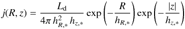 (4)with Ld the disc luminosity, hR, ∗ the radial scalelength and hz, ∗ the vertical scaleheight. For the stellar bulge, we assume the following 3D distribution,
  (5)where
  (6)is the spheroidal radius and
  is the Sérsic function, defined as the normalized 3D luminosity density corresponding to a Sérsic surface brightness profile, i.e. This function can only be expressed in analytical form using special functions (Mazure & Capelato 2002; Baes & Gentile 2011; Baes & van Hese 2011). Our bulge model has four free parameters: the bulge luminosity Lb, the effective radius Re, the Sérsic index n and the intrinsic flattening q.
The dust in the model is also distributed as a double-exponential disc, similar to the stellar disc,  (7)with Md the total dust mass, and hR,d and hz,d the radial scalelength and vertical scaleheight of the dust respectively. The central face-on optical depth, often used as an alternative to express the dust content, is easily calculated
  (8)where κ is the extinction coefficient of the dust.
In total, this 3D model has 10 free parameters, to which the inclination i of the galaxy with respect to the line of sight should be added as an 11th parameter. To construct our reference model, we selected realistic values for all parameters, based on average properties of the stellar discs, bulges and dust discs in spiral galaxies (Xilouris et al. 1999; Kregel et al. 2002; Hunt et al. 2004; Bianchi 2007; Cortese et al. 2012). The set of parameters is listed in the third column of Table 1. We constructed a V-band image on which we will test the FitSKIRT code by running the SKIRT code in monochromatic mode on this model, fully taking into account absorption and multiple anisotropic scattering. The optical properties of the dust were taken from Draine & Li (2007). The resulting input image is shown in the top panel of Fig. 6. It is 500 × 100 pixels in size, has a pixel scale of 100 pc/pixel and the reference frame was created using 107 photon packages.
We now apply the FitSKIRT code with the same parameter model to this artificial test image and investigate whether we can recover the initial parameters of the model. We proceed in different steps, first keeping a number of parameters in the model fixed to their input value and gradually increasing the number of free parameters.
3.2. One free parameter
To do some first basic testing with FitSKIRT, no luminosity fitting is used on any of the images. Apart from the dust mass Md all parameters are fixed and set to the same of the simulated image. We let FitSKIRT search for the best fitting model with the dust mass ranging between 5 × 10⁶ and 1.25 × 10⁸ M⊙. Note that this interval is not symmetric with respect to the model input value of 4 × 10⁷ M⊙, which makes it slightly more difficult to determine the real value.
Figure 4 shows the evolution of a population of 100 individuals through 20 generations with a mutation probability of 10% and a crossover rate of 70%. In fact, when using genomes with only one free parameter, the crossover rate becomes quite meaningless. This is because the crossover between two different genomes will result in an offspring that is essentially exactly the same as the best of the parent genomes. This duplication will, however, still result in a faster convergence since the mutation around those genomes will generally be in a better area than around a random position. FitSKIRT recovers a dust mass of (4.00 ± 0.02) × 107 M⊙, exactly equal to the dust mass of the input model. This figure shows that the parameter space is indeed asymmetrical around the true value (indicated by the red line) and that the entire population is gradually shifting towards the optimal value.
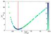 |
Fig. 4 Evolution of the determination of the dust mass in the FitSKIRT test simulation with one free parameter. The plot shows the distribution of the χ2 value for each of the 100 individuals for 20 generations. The colors represent the different generations and the input value is indicated by a red line. |
3.3. Three free parameters
As a second step we considere the case where we fitted three free parameters, more specifically the three parameters defining the dust distribution: the dust mass Md, the radial scale length hR,d and vertical scale height hz,d. The dust parameters are hard to determine individually since they have to be determined directly from the dust lane. The stellar parameters on the other hand are more easily determined and constrained in a larger region outside the dust lane. The problem is close to being degenerate when we look at the dust scale length and dust mass in exact edge-on, since changing them will roughly affect the same pixels.
We consider a wide possible range for the free parameters: the dust scale length was searched between 3 and 9 kpc, the scale height between 50 and 600 pc and for the dust mass we considered a range between 5 × 10⁶ and 1.25 × 10⁸ M⊙. In Fig. 5 we can see the evolution of a population consisting of 100 individuals through 20 generations in the hR,d versus hz,d and the hR,d versus Md projections of the 3D parameter space. For now we only consider a crossover of 70% and disable the mutation so we can take a closer look at the global optimization process. As we can see the entire population slowly converges until, in the end, it is located entirely around the actual value. This is indeed what we would expect from a global optimization process. The final best fit values are summarized in the fifth column of Table 1. With only three free parameters, FitSKIRT is still able to converge towards the exact values within the uncertainties. Notice that out of all parameters, the dust scale length hR,d is the hardest to constrain for edge-on galaxies. The values can be constrained even more if we use the mutation operator because the search space is then investigated in a multi-dimensional normal distribution around these individuals. Since in the end most individuals reside in the same area, this area will be sampled quite well.
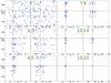 |
Fig. 5 Evolution of the dust parameters for a population of 100 individuals for the test model with three free parameters. The different panels show the position of each individual in the hR,d versus hz,d and the hR,d versus Md projections of the 3D parameter space, for different generations (indicated by the green numbers on the top of each panel). The input values of the parameters are indicated by red lines. |
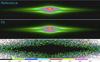 |
Fig. 6 Results of the FitSKIRT radiative transfer fit to the artificial edge-on spiral galaxy with 11 free parameters. The reference input V-band image is shown on the top panel, the FitSKIRT solution is shown in the middle panel, and the bottom panel represents the residual frame. |
3.4. Eleven free parameters
As a final test, FitSKIRT was used to fit all 11 parameters of the model described in Sect. 3.1. This corresponds to a full 10 + 1 dimensional optimization problem (10 parameters fitted by the genetic algorithm and the total luminosity determined independently by a golden section search). The appendix section also contains a comparison between genetic algorithms, Levenberg-Marquardt and downhill-simplex method for this specific case. In order to accommodate the significant increase of the parameter space, we also changed the parameters of the genetic algorithm fit: we consider 100 generations of 250 individuals each and set the mutation rate to 5% and the crossover rate to 60%. We also have to keep in mind that larger populations are less sensitive to noise (Goldberg et al. 1991).
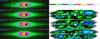 |
Fig. 7 Radiative transfer model fits to a V-band image of NGC 4013. The top right panel shows the observed image, the subsequent rows show the best fitting SKIRT image, and the models by Bianchi (2007) and Xilouris et al. (1999). The panels on the right-hand side show the residual images corresponding to these models. |
The result of this fitting exercise is given in the sixth column of Table 1. These results are also shown graphically in Fig. 6. The central panel shows the simulated image of our best fitting model, to be compared with the reference image shown on the top panel. The bottom panel gives the residual image. This figure clearly shows that the reference image is reproduced quite accurately by FitSKIRT and the residual frame shows a maximum of 10% discrepancy in most of the pixels, which is quite impressive considering the complexity of the problem and vastness of the parameter space. Apart from a good global fit, the individual parameters are also very well recovered: we can recover all fitted parameters within the 1σ uncertainty interval (only the bulge effective radius is just outside this one standard deviation range). The uncertainty estimates are also useful to get more insight in which parameters are easily constrained and which are not. From Table 1 it is clear that the dust scale length and dust mass are the hardest to constrain. These parameters are close to degenerate when fitting edge-on spiral galaxies as the fitting routine is most sensitive to the edge-on optical depth, i.e. the dust column within the plane of the galaxy. Both a dust distribution with a large dust mass but a small scale length and a distribution with a small dust mass and a large scale length can conspire to give similar edge-on optical depths.
4. Application on observed data: NGC 4013
In this final section we apply FitSKIRT to recover the intrinsic distribution of stars and dust in the edge-on spiral galaxy NGC 4013. Located at a distance of about 18.6 Mpc (Willick et al. 1997; Russell 2002; Tully et al. 2009) and with a D25 diameter of 5.2 arcmin, this galaxy is one of the most prominent edge-on spiral galaxies. It is very close to exactly edge-on and its dust lane can be traced to the edges of the galaxy. Conspicuous properties of this galaxy are its box- or peanut-shaped bulge (Kormendy & Illingworth 1982; Jarvis 1986; García-Burillo et al. 1999) and the warp in the gas and stellar distribution (Bottema et al. 1987; Florido et al. 1991; Bottema 1995, 1996; Saha et al. 2009). The main reason why we selected this particular galaxy is that it has been modelled before twice using independent radiative transfer fitting methods, namely by Xilouris et al. (1999) and Bianchi (2007). This allows a direct comparison of the FitSKIRT algorithm with other fitting procedures in a realistic context.
We use a V-band image of NGC 4013, taken with the Telescopio Nazionale Galileo (TNG). Full details on the observations and data reduction can be found in Bianchi (2007). The image can be found in the top left panel of Fig. 7. We apply the FitSKIRT program to reproduce this V-band image, in a field of approximatively 5.5′ × 1′. The same model is used as the test simulations discussed in Sect. 3, i.e. a double-exponential disc and a flattened Sérsic bulge for the stellar distribution and a double-exponential disc for the dust distribution. We do not fix any parameters, i.e. we are again facing a 10 + 1 dimensional optimization problem. The genetic algorithm parameters are the same as for the test problem, i.e. 100 generations of 250 individuals each, a mutation rate of 5% and a crossover rate of 60%.
The results of our FitSKIRT fit are given in the third column of Table 2. We find a V-band face-on optical depth of almost unity, corresponding to a dust mass of 9.9 × 10⁶ M⊙. In Fig. 7 we plot the best fit to the observed V-band image of NGC 4013 and its residuals. These two panels show that our FitSKIRT model provides a very satisfactory fit to the observed image: the residuals between the image and fit are virtually everywhere smaller than 20%. The main exceptions where the fit is less accurate are the central-left region of the disc which contains discernible clumpy structures (which are obviously not properly described by our simple analytical model) and the top-right region, which is due to the warping of the disc in NGC 4013. The quality of our FitSKIRT fit is quantified in Fig. 8, where we plot the cumulative distribution of the residual values of the innermost 15 000 pixels in the fit, i.e. the number of pixels with a residual smaller than a certain percentage. We see that half of the pixels have a residual less than 15%, and almost 90% of the pixels have a residual less than 50%.
In the last two columns of Table 2 we list the parameters found by Xilouris et al. (1999) and Bianchi (2007), scaled to our assumed distance of 18.6 Mpc and considering the same value for the dust extinction coefficient κ, necessary to convert optical depths to dust masses as in Eq. (8). In Fig. 7 we also compare the images and their residuals for the models by Xilouris et al. (1999) and Bianchi (2007) with the FitSKIRT model. We reconstructed these models by taking the parameters from Table 2 and build a V-band model image of the galaxy with SKIRT. The same quantitative analysis on the residual frames as for the FitSKIRT solution is also plotted in Fig. 8.
Parameters of the intrinsic distribution of stars and dust in NGC 4013 as obtained by FitSKIRT, by Bianchi (2007) and by Xilouris et al. (1999).
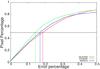 |
Fig. 8 The cumulative distribution of the number of pixels with a residual smaller than a given percentage for the three model fits to the V-band image of NGC 4013. The green, red and blue solid lines correspond to the FitSKIRT model, the Xilouris et al. (1999) model and the Bianchi (2007) model respectively. The dashed horizontal line corresponds to half of the total number of pixels. |
Looking at the model fits and their residuals, it is immediately clear that the three models are very similar. The largest deviations from the observed image are found at the same locations for the three models and hence seem to be due to impossibility of our smooth analytical model to represent the true distribution of stars and dust in the galaxies rather than due to the fitting techniques. Figure 8 seems to suggest that the FitSKIRT solution provides a slightly better overall fit to the image, but this judgement might be biased by the fact that we reproduced the other models with our SKIRT code (their model might be slightly different). Looking at the model parameters in Table 2, it is clear that the most prominent differences between the three models are the different values of the face-on optical depth and the dust scale length. This finding is not surprising given that we already found in Sects. 3.3 and 3.4 that these parameters are the hardest to constrain. This also corresponds to what (Bianchi 2007) states as the reason for the high optical depth: the large optical depth is compensated by the smaller scale length of the dust disk.
An important aspect to take into account when comparing the results from the three models is the slight variations in the model setup and the strong differences in the radiative transfer calculations and the fitting techniques. Xilouris et al. (1999) used an approximate analytical method to solve the radiative transfer, based on the so-called method of scattered intensities pioneered by Henyey (1937) and subsequently perfectionized and applied by Kylafis & Bahcall (1987), Xilouris et al. (1997, 1998, 1999), Baes & Dejonghe (2001a), Popescu et al. (2000, 2011) and Möllenhoff et al. (2006). To do the fitting, they used a Levenberg-Marquardt algorithm. They used an approximation of a de Vaucouleurs model to fit the bulge and excluded the central 200 pc from the fit. The modelling of NGC 4013 by Bianchi (2007) on the other hand was based on the Monte Carlo code TRADING (Bianchi et al. 1996, 2000; Bianchi 2008). For the actual fitting, he used a combination of the Levenberg-Marquardt algorithm (applied to model without scattering) and the amoeba downhill simplex algorithm. He also used an approximation of a de Vaucouleurs model to fit the bulge. Given these differences from the FitSKIRT approach, the agreement between the parameters of the three models is very satisfactory.
5. Discussion and conclusions
In this paper, we have presented the FitSKIRT code, a tool designed to recover the spatial distribution of stars and dust from fitting radiative transfer models to UV, optical or near-infrared images. It combines a state-of-the-art Monte Carlo radiative transfer code with the power of genetic algorithms to perform the actual fitting. The noise handling properties together with the ability to uniformly investigate and optimize a complex parameter space, make genetic algorithms an ideal candidate to use in combination with a Monte Carlo radiative transfer code. Using a standard but challenging optimization problem, we have demonstrated that the specific genetic algorithm library chosen for FitSKIRT, GAlib, is reliable and efficient. We could overcome the main shortcoming of the genetic algorithm approach, the lack of appropriate error bars on the model parameters, by deriving the spread of the individual parameters when applying the optimization process several times with different initial conditions.
The FitSKIRT program was tested on an artificial reference image of a dusty edge-on spiral galaxy model created by the SKIRT radiative transfer code. This reference image was fed to the FitSKIRT code in a series of tests with an increasing number of free parameters. The reliability of the code was evaluated by investigating the residual frames as well as the recovery of the input model parameters. From both the one and three parameters fittings we concluded that the optimization process is stable enough and does not converge too fast towards local extrema. FitSKIRT recovered the input parameters very well, even for the full problem in which all 11 parameters of the input model were left unconstrained.
As a final test, the FitSKIRT method was applied to determine the physical parameters of the stellar and dust distribution in the edge-on spiral galaxy NGC 4013 from a single V-band image. Looking at the cumulative distribution of the number of pixels in the residual map, we found that FitSKIRT was able to fit half of the pixels with a residual of less than 15% and almost 90% of the pixels with a residual of less than 50%. Given that the image of NGC 4013 clearly shows a number of regions that cannot be reproduced by a smooth model (due to obvious clumping in the dust lane and a warp in the stellar and gas distribution), these statistics are very encouraging. The values of the fitted parameters and the quality of the fit were compared with similar but completely independent radiative transfer fits done by Xilouris et al. (1999) and Bianchi (2007). There are some deviations between the results, and we argue that these can be explained by the degeneracy between the dust scale length and face-on optical depth, and the differences in the model setup, radiative transfer technique and optimization strategy. In general, the agreement between the parameters of the three models is very satisfactory.
We have demonstrated in this paper that the FitSKIRT code is capable of recovering the intrinsic parameters of the stellar and dust distribution of edge-on spiral galaxies by fitting radiative transfer models to an observed optical image. A future extension we foresee is to include images at different wavelengths in our modelling procedure. In its most obvious form, one could run FitSKIRT independently on different images, and use the results obtained at different wavelengths to study the wavelength dependence of the stars and dust (Xilouris et al. 1997, 1998, 1999; Bianchi 2007). In particular, the wavelength dependence of the optical depth, i.e. the intrinsic extinction curve, is a strong diagnostic for the size distribution and the composition of the dust grains (Greenberg & Chlewicki 1983; Desert et al. 1990; Li & Greenberg 1997; Weingartner & Draine 2001; Clayton et al. 2003; Zubko et al. 2004). One step beyond this is an expansion of FitSKIRT in which images at different wavelengths are fitted simultaneously, and a single model is sought that provides the best overall fit to a set of UV/optical/NIR images. A so-called oligochromatic radiative transfer fitting could disentangle some of the degeneracies which monochromatic fitting procedures have to deal with, and can also be used to predict the corresponding FIR/submm emission of the system (Popescu et al. 2000; Baes et al. 2010; De Looze et al. 2012a,b).
The main goal of the paper was to present the philosophy and ingredients behind the FitSKIRT code, and to demonstrate that it is capable of determining the structural parameters of the stellar and dust distribution in edge-on spiral galaxies using UV/optical/NIR imaging data. Obviously, we have the intention to also apply this code to real data to investigate the physical properties of galaxies. As the optimization process in FitSKIRT can cover a large parameter space and the code is almost fully automated (which implies minimal human intervention and hence bias), it is a very versatile tool and is ready to be applied to a variety of galaxies, including larger sets of observational data.
We are currently applying the code to a set of large edge-on spiral galaxies in order to recover the detailed distribution of stars and dust. Our main motivation is to investigate whether the amount of dust observed in the UV/optical/NIR window agrees with the dust masses derived from MIR/FIR/submm observations, which has been subject of some debate in recent years (Misiriotis et al. 2001, 2006; Alton et al. 2004; Bianchi 2008; Baes et al. 2010; Popescu et al. 2011; MacLachlan et al. 2011). Major problems that have hampered much progress in this topic in the past were the limited wavelength coverage and sensitivity of the FIR/submm observations and the small number of galaxies for which such observations and detailed radiative transfer models were available. These problems are now being cured. On the one hand, we now have a powerful tool available to fit optical/NIR images in an automated way without the need for and the bias from human intervention. On the other hand, Spitzer and Herschel have now provided us with deep imaging observations of significant numbers of nearby edge-on spiral galaxies at various FIR/submm wavelengths (e.g. Bianchi & Xilouris 2011; Holwerda et al. 2012; De Looze et al. 2012a,b; Ciesla et al. 2012; Verstappen et al. 2012).
We have focused our attention here on edge-on spiral galaxies, which are the obvious and most popular candidates for radiative transfer modelling because of their prominent dust lanes. However, these are not the only targets on which FitSKIRT could be applied. In principle, the fitting routine can be applied on any geometry, but for monochromatic fitting the dust parameters can only be constrained for galaxies with a clear and regular signature of dust extinction. Apart from edge-on spiral galaxies, an interesting class of galaxies are early-type galaxies which often show regular and large-scale dust lanes (e.g. Bertola & Galletta 1978; Hawarden et al. 1981; Ebneter & Balick 1985; Patil et al. 2007; Finkelman et al. 2008, 2010). We plan to apply our FitSKIRT modelling in the future to a sample of dust-lane early-type galaxies, primarily focusing on those galaxies that have been mapped at FIR/submm wavelengths (e.g. Smith et al. 2012b).
Other applications are possible and the authors welcome suggestions from interested readers.
A possible explanation for this difference might be the generational versus the steady state reproduction. It has to be noted, however, that the PIKAIA results we quote are from Charbonneau (1995). Many researchers have adapted and updated the PIKAIA code since 1995, probably also increasing its efficiency.
Acknowledgments
We thank Karl Gordon, Jürgen Steinacker, Ilse De Looze, Joris Verstappen, Simone Bianchi and Manolis Xilouris, for stimulating discussions on radiative transfer modelling. We would like to express our gratitude to Matthew Wall for the creation and sharing of the GAlib library. G.D.G. is supported by the Flemish Fund for Scientific Research (FWO-Vlaanderen). J.F., M.B. and P.C. acknowledge the financial support of the Belgian Science Policy Office.
References
- Alton, P. B., Xilouris, E. M., Misiriotis, A., Dasyra, K. M., & Dumke, M. 2004, A&A, 425, 109 [NASA ADS] [CrossRef] [EDP Sciences] [Google Scholar]
- Baes, M. 2008, MNRAS, 391, 617 [NASA ADS] [CrossRef] [Google Scholar]
- Baes, M., & Dejonghe, H. 2001a, MNRAS, 326, 722 [NASA ADS] [CrossRef] [Google Scholar]
- Baes, M., & Dejonghe, H. 2001b, MNRAS, 326, 733 [NASA ADS] [CrossRef] [Google Scholar]
- Baes, M., & Dejonghe, H. 2002, MNRAS, 335, 441 [NASA ADS] [CrossRef] [Google Scholar]
- Baes, M., & Gentile, G. 2011, A&A, 525, A136 [NASA ADS] [CrossRef] [EDP Sciences] [Google Scholar]
- Baes, M., & van Hese, E. 2011, A&A, 534, A69 [NASA ADS] [CrossRef] [EDP Sciences] [Google Scholar]
- Baes, M., Davies, J. I., Dejonghe, H., et al. 2003, MNRAS, 343, 1081 [NASA ADS] [CrossRef] [Google Scholar]
- Baes, M., Stamatellos, D., Davies, J. I., et al. 2005, New A, 10, 523 [Google Scholar]
- Baes, M., Fritz, J., Gadotti, D. A., et al. 2010, A&A, 518, L39 [NASA ADS] [CrossRef] [EDP Sciences] [Google Scholar]
- Baes, M., Verstappen, J., De Looze, I., et al. 2011, ApJS, 196, 22 [NASA ADS] [CrossRef] [Google Scholar]
- Baier, A., Kerschbaum, F., & Lebzelter, T. 2010, A&A, 516, A45 [NASA ADS] [CrossRef] [EDP Sciences] [Google Scholar]
- Bendo, G. J., Wilson, C. D., Pohlen, M., et al. 2010, A&A, 518, L65 [NASA ADS] [CrossRef] [EDP Sciences] [Google Scholar]
- Bendo, G. J., Boselli, A., Dariush, A., et al. 2012, MNRAS, 419, 1833 [NASA ADS] [CrossRef] [Google Scholar]
- Bertola, F., & Galletta, G. 1978, ApJ, 226, L115 [NASA ADS] [CrossRef] [Google Scholar]
- Bianchi, S. 2007, A&A, 471, 765 [NASA ADS] [CrossRef] [EDP Sciences] [Google Scholar]
- Bianchi, S. 2008, A&A, 490, 461 [NASA ADS] [CrossRef] [EDP Sciences] [Google Scholar]
- Bianchi, S., & Xilouris, E. M. 2011, A&A, 531, L11 [NASA ADS] [CrossRef] [EDP Sciences] [Google Scholar]
- Bianchi, S., Ferrara, A., & Giovanardi, C. 1996, ApJ, 465, 127 [NASA ADS] [CrossRef] [Google Scholar]
- Bianchi, S., Davies, J. I., & Alton, P. B. 2000, A&A, 359, 65 [NASA ADS] [Google Scholar]
- Bianchi, S., Gonçalves, J., Albrecht, M., et al. 2003, A&A, 399, L43 [NASA ADS] [CrossRef] [EDP Sciences] [Google Scholar]
- Bjorkman, J. E., & Wood, K. 2001, ApJ, 554, 615 [NASA ADS] [CrossRef] [Google Scholar]
- Bottema, R. 1995, A&A, 295, 605 [NASA ADS] [Google Scholar]
- Bottema, R. 1996, A&A, 306, 345 [NASA ADS] [Google Scholar]
- Bottema, R., Shostak, G. S., & van der Kruit, P. C. 1987, Nature, 328, 401 [NASA ADS] [CrossRef] [Google Scholar]
- Byun, Y. I., Freeman, K. C., & Kylafis, N. D. 1994, ApJ, 432, 114 [NASA ADS] [CrossRef] [Google Scholar]
- Cantó, J., Curiel, S., & Martínez-Gómez, E. 2009, A&A, 501, 1259 [NASA ADS] [CrossRef] [EDP Sciences] [Google Scholar]
- Charbonneau, P. 1995, ApJS, 101, 309 [NASA ADS] [CrossRef] [Google Scholar]
- Ciesla, L., Boselli, A., Smith, M. W. L., et al. 2012, A&A, 543, A161 [NASA ADS] [CrossRef] [EDP Sciences] [Google Scholar]
- Clayton, G. C., Wolff, M. J., Sofia, U. J., Gordon, K. D., & Misselt, K. A. 2003, ApJ, 588, 871 [NASA ADS] [CrossRef] [Google Scholar]
- Cortese, L., Ciesla, L., Boselli, A., et al. 2012, A&A, 540, A52 [NASA ADS] [CrossRef] [EDP Sciences] [Google Scholar]
- De Looze, I., Baes, M., Zibetti, S., et al. 2010, A&A, 518, L54 [NASA ADS] [CrossRef] [EDP Sciences] [Google Scholar]
- De Looze, I., Baes, M., Bendo, G. J., et al. 2012a, MNRAS, 427, 2797 [NASA ADS] [CrossRef] [Google Scholar]
- De Looze, I., Baes, M., Fritz, J., & Verstappen, J. 2012b, MNRAS, 419, 895 [NASA ADS] [CrossRef] [Google Scholar]
- Desert, F.-X., Boulanger, F., & Puget, J. L. 1990, A&A, 237, 215 [NASA ADS] [Google Scholar]
- di Bartolomeo, A., Barbaro, G., & Perinotto, M. 1995, MNRAS, 277, 1279 [NASA ADS] [CrossRef] [Google Scholar]
- Disney, M., Davies, J., & Phillipps, S. 1989, MNRAS, 239, 939 [NASA ADS] [CrossRef] [Google Scholar]
- Draine, B. T., & Li, A. 2007, ApJ, 657, 810 [NASA ADS] [CrossRef] [Google Scholar]
- Dupac, X., Bernard, J.-P., Boudet, N., et al. 2003, A&A, 404, L11 [NASA ADS] [CrossRef] [EDP Sciences] [Google Scholar]
- Ebneter, K., & Balick, B. 1985, AJ, 90, 183 [NASA ADS] [CrossRef] [Google Scholar]
- Finkelman, I., Brosch, N., Kniazev, A. Y., et al. 2008, MNRAS, 390, 969 [NASA ADS] [CrossRef] [Google Scholar]
- Finkelman, I., Brosch, N., Kniazev, A. Y., et al. 2010, MNRAS, 409, 727 [NASA ADS] [CrossRef] [Google Scholar]
- Fletcher, S. T., Chaplin, W. J., & Elsworth, Y. 2003, MNRAS, 346, 825 [NASA ADS] [CrossRef] [Google Scholar]
- Florido, E., Prieto, M., Battaner, E., et al. 1991, A&A, 242, 301 [NASA ADS] [Google Scholar]
- Foyle, K., Wilson, C. D., Mentuch, E., et al. 2012, MNRAS, 421, 2917 [NASA ADS] [CrossRef] [Google Scholar]
- Fritz, J., Gentile, G., Smith, M. W. L., et al. 2012, A&A, 546, A34 [NASA ADS] [CrossRef] [EDP Sciences] [Google Scholar]
- Galametz, M., Kennicutt, R. C., Albrecht, M., et al. 2012, MNRAS, 425, 763 [NASA ADS] [CrossRef] [Google Scholar]
- Galliano, F., Hony, S., Bernard, J.-P., et al. 2011, A&A, 536, A88 [NASA ADS] [CrossRef] [EDP Sciences] [Google Scholar]
- García-Burillo, S., Combes, F., & Neri, R. 1999, A&A, 343, 740 [NASA ADS] [Google Scholar]
- Goldberg, D. E. 1989, Genetic Algorithms in Search, Optimization and Machine Learning, 1st edn. (Boston, MA, USA: Addison-Wesley Longman Publishing Co., Inc.) [Google Scholar]
- Goldberg, D. E., Deb, K., & Clark, J. H. 1991, Complex Systems, 6, 333 [Google Scholar]
- Gomez, H. L., Baes, M., Cortese, L., et al. 2010, A&A, 518, L45 [NASA ADS] [CrossRef] [EDP Sciences] [Google Scholar]
- Gordon, K. D., Misselt, K. A., Witt, A. N., & Clayton, G. C. 2001, ApJ, 551, 269 [NASA ADS] [CrossRef] [Google Scholar]
- Greenberg, J. M., & Chlewicki, G. 1983, ApJ, 272, 563 [NASA ADS] [CrossRef] [Google Scholar]
- Hawarden, T. G., Longmore, A. J., Tritton, S. B., Elson, R. A. W., & Corwin, Jr., H. G. 1981, MNRAS, 196, 747 [NASA ADS] [CrossRef] [Google Scholar]
- Henyey, L. G. 1937, ApJ, 85, 107 [NASA ADS] [CrossRef] [Google Scholar]
- Holwerda, B. W., Bianchi, S., Böker, T., et al. 2012, A&A, 541, L5 [NASA ADS] [CrossRef] [EDP Sciences] [Google Scholar]
- Howell, S. B. 2006, Handbook of CCD astronomy, 2nd edn. (Cambridge University Press) [Google Scholar]
- Hunt, L. K., Pierini, D., & Giovanardi, C. 2004, A&A, 414, 905 [NASA ADS] [CrossRef] [EDP Sciences] [Google Scholar]
- Inoue, A. K. 2005, MNRAS, 359, 171 [NASA ADS] [CrossRef] [Google Scholar]
- Jarvis, B. J. 1986, AJ, 91, 65 [NASA ADS] [CrossRef] [Google Scholar]
- Jonsson, P. 2006, MNRAS, 372, 2 [NASA ADS] [CrossRef] [Google Scholar]
- Juvela, M., & Ysard, N. 2012a, A&A, 541, A33 [NASA ADS] [CrossRef] [EDP Sciences] [Google Scholar]
- Juvela, M., & Ysard, N. 2012b, A&A, 539, A71 [NASA ADS] [CrossRef] [EDP Sciences] [Google Scholar]
- Kelly, B. C., Shetty, R., Stutz, A. M., et al. 2012, ApJ, 752, 55 [NASA ADS] [CrossRef] [Google Scholar]
- Kormendy, J., & Illingworth, G. 1982, ApJ, 256, 460 [NASA ADS] [CrossRef] [Google Scholar]
- Kramer, C., Richer, J., Mookerjea, B., Alves, J., & Lada, C. 2003, A&A, 399, 1073 [NASA ADS] [CrossRef] [EDP Sciences] [Google Scholar]
- Kregel, M., van der Kruit, P. C., & de Grijs, R. 2002, MNRAS, 334, 646 [NASA ADS] [CrossRef] [Google Scholar]
- Kylafis, N. D., & Bahcall, J. N. 1987, ApJ, 317, 637 [NASA ADS] [CrossRef] [Google Scholar]
- Larsen, J. A., & Humphreys, R. M. 2003, AJ, 125, 1958 [NASA ADS] [CrossRef] [Google Scholar]
- Levenberg, K. 1944, Q. Appl. Math, 2, 164 [Google Scholar]
- Li, A., & Greenberg, J. M. 1997, A&A, 323, 566 [NASA ADS] [Google Scholar]
- Liesenborgs, J., De Rijcke, S., & Dejonghe, H. 2006, MNRAS, 367, 1209 [NASA ADS] [CrossRef] [Google Scholar]
- Lucy, L. B. 1999, A&A, 344, 282 [NASA ADS] [Google Scholar]
- MacLachlan, J. M., Matthews, L. D., Wood, K., & Gallagher, J. S. 2011, ApJ, 741, 6 [NASA ADS] [CrossRef] [Google Scholar]
- Marquardt, D. W. 1963, SIAM J. Appl. Math., 11, 431 [Google Scholar]
- Mattila, K. 1970, A&A, 9, 53 [NASA ADS] [Google Scholar]
- Mazure, A., & Capelato, H. V. 2002, A&A, 383, 384 [NASA ADS] [CrossRef] [EDP Sciences] [Google Scholar]
- Meixner, M., Galliano, F., Hony, S., et al. 2010, A&A, 518, L71 [NASA ADS] [CrossRef] [EDP Sciences] [Google Scholar]
- Metcalfe, T. S., Nather, R. E., & Winget, D. E. 2000, ApJ, 545, 974 [NASA ADS] [CrossRef] [Google Scholar]
- Misiriotis, A., Popescu, C. C., Tuffs, R., & Kylafis, N. D. 2001, A&A, 372, 775 [NASA ADS] [CrossRef] [EDP Sciences] [Google Scholar]
- Misiriotis, A., Xilouris, E. M., Papamastorakis, J., Boumis, P., & Goudis, C. D. 2006, A&A, 459, 113 [NASA ADS] [CrossRef] [EDP Sciences] [Google Scholar]
- Mitchell, M. 1998, An Introduction to Genetic Algorithms (Complex Adaptive Systems), 3rd edn. (A Bradford Book) [Google Scholar]
- Möllenhoff, C., Popescu, C. C., & Tuffs, R. J. 2006, A&A, 456, 941 [NASA ADS] [CrossRef] [EDP Sciences] [Google Scholar]
- Mortara, L., & Fowler, A. 1981, in SPIE Conf. Ser., 290, 28 [Google Scholar]
- Nelder, J. A., & Mead, R. 1965, Comput. J., 7, 308 [CrossRef] [Google Scholar]
- Nesseris, S., & García-Bellido, J. 2012, J. Cosmol. Astropart. Phys., 11, 33 [Google Scholar]
- Nesseris, S., & Shafieloo, A. 2010, MNRAS, 408, 1879 [NASA ADS] [CrossRef] [Google Scholar]
- Newberry, M. V. 1991, PASP, 103, 122 [NASA ADS] [CrossRef] [Google Scholar]
- Patil, M. K., Pandey, S. K., Sahu, D. K., & Kembhavi, A. 2007, A&A, 461, 103 [NASA ADS] [CrossRef] [EDP Sciences] [Google Scholar]
- Pilbratt, G. L., Riedinger, J. R., Passvogel, T., et al. 2010, A&A, 518, L1 [CrossRef] [EDP Sciences] [Google Scholar]
- Popescu, C. C., Misiriotis, A., Kylafis, N. D., Tuffs, R. J., & Fischera, J. 2000, A&A, 362, 138 [NASA ADS] [Google Scholar]
- Popescu, C. C., Tuffs, R. J., Dopita, M. A., et al. 2011, A&A, 527, A109 [NASA ADS] [CrossRef] [EDP Sciences] [Google Scholar]
- Press, W. H., Teukolsky, S. A., Vetterling, W. T., & Flannery, B. P. 1992, Numerical recipes in FORTRAN. The art of scientific computing, 2nd edn. (Cambridge University Press) [Google Scholar]
- Rajpaul, V. 2012a, MNRAS, 427, 1755 [NASA ADS] [CrossRef] [Google Scholar]
- Rajpaul, V. 2012b [arXiv:1202.1643] [Google Scholar]
- Robitaille, T. P. 2011, A&A, 536, A79 [NASA ADS] [CrossRef] [EDP Sciences] [Google Scholar]
- Robitaille, T. P., Whitney, B. A., Indebetouw, R., & Wood, K. 2007, ApJS, 169, 328 [NASA ADS] [CrossRef] [Google Scholar]
- Russell, D. G. 2002, ApJ, 565, 681 [NASA ADS] [CrossRef] [Google Scholar]
- Saha, K., de Jong, R., & Holwerda, B. 2009, MNRAS, 396, 409 [NASA ADS] [CrossRef] [Google Scholar]
- Sahinler, S., & Topuz, D. 2007, J. Appl. Quant. Methods, 408, 188 [Google Scholar]
- Schechtman-Rook, A., Bershady, M. A., & Wood, K. 2012, ApJ, 746, 70 [NASA ADS] [CrossRef] [Google Scholar]
- Shetty, R., Kauffmann, J., Schnee, S., & Goodman, A. A. 2009, ApJ, 696, 676 [NASA ADS] [CrossRef] [Google Scholar]
- Shirley, Y. L., Huard, T. L., Pontoppidan, K. M., et al. 2011, ApJ, 728, 143 [NASA ADS] [CrossRef] [Google Scholar]
- Smith, M. W. L., Eales, S. A., Gomez, H. L., et al. 2012a, ApJ, 756, 40 [NASA ADS] [CrossRef] [Google Scholar]
- Smith, M. W. L., Gomez, H. L., Eales, S. A., et al. 2012b, ApJ, 748, 123 [NASA ADS] [CrossRef] [Google Scholar]
- Stalevski, M., Fritz, J., Baes, M., Nakos, T., & Popović, L. Č. 2011, Balt. Astron., 20, 490 [NASA ADS] [Google Scholar]
- Stalevski, M., Fritz, J., Baes, M., Nakos, T., & Popović, L. Č. 2012, MNRAS, 420, 2756 [NASA ADS] [CrossRef] [Google Scholar]
- Steinacker, J., Bacmann, A., Henning, T., Klessen, R., & Stickel, M. 2005, A&A, 434, 167 [NASA ADS] [CrossRef] [EDP Sciences] [MathSciNet] [Google Scholar]
- Theis, C., & Kohle, S. 2001, A&A, 370, 365 [NASA ADS] [CrossRef] [EDP Sciences] [Google Scholar]
- Tully, R. B., Rizzi, L., Shaya, E. J., et al. 2009, AJ, 138, 323 [NASA ADS] [CrossRef] [Google Scholar]
- Veneziani, M., Ade, P. A. R., Bock, J. J., et al. 2010, ApJ, 713, 959 [NASA ADS] [CrossRef] [Google Scholar]
- Verstappen, J., Baes, M., Fritz, J., et al. 2012, MNRAS, submitted [Google Scholar]
- Vidal, E., & Baes, M. 2007, Balt. Astron., 16, 101 [Google Scholar]
- Wall, M. 1996, Ph.D. Thesis, Mechanical Engineering Department, Massachusetts Institute of Technology [Google Scholar]
- Weingartner, J. C., & Draine, B. T. 2001, ApJ, 548, 296 [NASA ADS] [CrossRef] [Google Scholar]
- Willick, J. A., Courteau, S., Faber, S. M., et al. 1997, ApJS, 109, 333 [NASA ADS] [CrossRef] [Google Scholar]
- Witt, A. N. 1977, ApJS, 35, 1 [NASA ADS] [CrossRef] [Google Scholar]
- Witt, A. N., Thronson, Jr., H. A., & Capuano, Jr. J. M. 1992, ApJ, 393, 611 [NASA ADS] [CrossRef] [Google Scholar]
- Xilouris, E. M., Kylafis, N. D., Papamastorakis, J., Paleologou, E. V., & Haerendel, G. 1997, A&A, 325, 135 [NASA ADS] [Google Scholar]
- Xilouris, E. M., Alton, P. B., Davies, J. I., et al. 1998, A&A, 331, 894 [NASA ADS] [Google Scholar]
- Xilouris, E. M., Byun, Y. I., Kylafis, N. D., Paleologou, E. V., & Papamastorakis, J. 1999, A&A, 344, 868 [NASA ADS] [Google Scholar]
- Xilouris, E. M., Tabatabaei, F. S., Boquien, M., et al. 2012, A&A, 543, A74 [NASA ADS] [CrossRef] [EDP Sciences] [Google Scholar]
- Yusef-Zadeh, F., Morris, M., & White, R. L. 1984, ApJ, 278, 186 [NASA ADS] [CrossRef] [Google Scholar]
- Zubko, V., Dwek, E., & Arendt, R. G. 2004, ApJS, 152, 211 [NASA ADS] [CrossRef] [Google Scholar]
Appendix A: Other optimization techniques
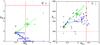 |
Fig. A.1 The function evaluations for both the Levenberg-Marquardt and downhill simplex method ranging from black (initial) to blue (DS) or green (LM) and the average path. The red lines indicate the values used to create the reference frame (Fig. 6). Left: the variation of the dust mass and the scale length of the dust disk. Right: the variation of the scale length and scale height of the stellar disk. |
As described in Sect. 2.2, the choice of genetic algorithms as our preferred optimization routine was driven by the nature of our problem: the minimization of a complex, numerical and noisy objective function in a large, multi-dimensional parameters space, characterized by several local minima. As we have demonstrated, the genetic algorithm approach turned out to be a powerful tool in this respect, and enabled us to reach our goals. In particular, concerning the problem of noisy objective functions, genetic algorithms are very effective: since they work on a population rather than iteratively on one point, that the random noise in the objective function is a much less determining factor in the final solution (Metcalfe et al. 2000; Larsen & Humphreys 2003). On the other hand, the method is not entirely free of drawbacks: compared to some other optimization routines, genetic algorithms have a relatively slow convergence rate on simple problems, and the error analysis is not easily treated in a natural way.
To further explore other possibilities and not limit ourselves to this one approach only, we have performed further tests adopting two other optimization schemes that have been used in radiative transfer fitting problems, namely the Levenberg-Marquardt and the downhill-simplex methods. Both methods were applied to the test case we have considered in Sect. 3.4, and their performance is compared to genetic algorithms. In the following we briefly describe these two routines and present the results of the comparison.
Appendix A.1: Levenberg-Marquardt method
The Levenberg-Marquardt algorithm or damped least-squares method (Levenberg 1944; Marquardt 1963) is an iterative optimization method, that uses the gradient of the objective function and a damping factor based on the local curvature to find the next step in the iteration towards the final solution. The Levenberg-Marquardt method is one of the most widely used methods for nonlinear optimization problems. It has been applied in inverse radiative transfer modelling by Xilouris et al. (1999) and Bianchi (2007). The choice of this algorithm was possible because the radiative transfer approach used by both was an (approximate) analytical model (Bianchi (2007) only used the Levenberg-Marquardt method for fits with ray-tracing radiative transfer simulations where scattering was taken into account). In that case, the gradient in the multi-dimensional parameter space only requires a modest computational effort and is free of random noise.
As we are dealing with a Monte Carlo radiative transfer code with a full inclusion of multiple anisotropic scattering, adapting this method was not trivial. In particular, the presence of Monte Carlo noise on the objective function evaluation makes the (numerical) calculation of the gradient difficult. In an attempt to overcome this problem we have combined two solutions:
-
we increase the number of photon packages in everyMonte Carlo simulation, so that the noise isreduced to a minimum but leads to computationally moredemanding simulations;
-
we calculate the gradient based on different different objective function evaluations in every parameter space dimension. This helps to mitigate both the high impact that the noise has on the gradient in regions close to the starting point, and also the unrealistic values that the gradient can yield when calculated on points located further away from the current position.
In our implementation, we found that the number objective function evaluations needed to make one single Levenberg-Marquardt step is around 70 for our optimization problem containing 11 free parameters (Sect. 3.4). Keeping in mind that we have to use a larger number of photon packages, one single Levenberg-Marquardt step is comparable to approximately 400 evaluations performed in the genetic algorithms approach, in terms of computational effort.
Appendix A.2: Downhill simplex method
The downhill simplex method, also known as Nelder-Mead method or amoeba method (Nelder & Mead 1965), is another commonly used non-linear optimization technique. The method iteratively refines the search space defined by an (N + 1)-dimensional simplex by replacing one of its defining points, typically the one with the worst objective function evaluation, with its reflection through the centroid of the remaining N points defining the simplex.
In relatively simple optimization problems, the downhill simplex method is known to have a relatively poor convergence, i.e. it is not efficient in the number of objective function evaluations necessary to find the extremum. On the positive side, the method only needs the evaluation of the objective function itself and does not require additional information on the parameter space or the calculation of gradients. Importantly, the method also works better with noisy objective functions compared to Levenberg-Marquardt. Hence, coupling a downhill simplex routing to a Monte Carlo radiative transfer code requires no additional adjustments as instead needed in the case of Levenberg-Marquardt. The downhill simplex method was used by Bianchi (2007) for the general case, i.e. for fits in which scattering was included (and hence Monte Carlo noise was present).
Appendix A.3: Results and comparison
When applying the Levenberg-Marquardt and downhill simplex algorithms to the problem discussed in Sect. 3.4, both methods are initialized in the same, randomly determined position and new evaluations are performed until there is no significant improvement in the values of the objective function. The left panel of Fig. A.1 shows the function evaluations (points) and the averaged path (lines) of the Levenberg-Marquardt (green) and downhill simpex (blue) methods for the dust mass and scale length of the dust disk, two parameters which are hard to constrain separately. The first evaluation – or starting point – is marked with a black open circle, while the “real” values are indicated by the red lines. The history of the function evaluations is colour coded (from black at the beginning to gradually green or blue, for the last evaluation).
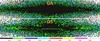 |
Fig. A.2 The residual frame of the reference image and the best fitting model as determined by the GA (top) and the repeatedly restarted Downhill Simplex method (bottom). The parameter values are listed in Table A.1. The green line in the bottom image is the result of slight inaccuracies in the reproduction of the dust lane. |
Figure A.1 visually demonstrates another fundamental complication of both the Levenberg-Marquardt and downhill simplex methods: they both fail to reach the area of the parameter space located closely to the true values. Even for parameters which are more easily determined, like the scale length and height of the stellar disk (see the right panel in Fig. A.1), the methods do not succeed at reaching the region around the true values. This, however, should not come as a surprise since both methods are known to be local rather than global optimization methods. This limitation can be partially overcome by repeatedly restarting the algorithm in a new random initial position. For the Levenberg-Marquardt method, this is simply unfeasible as it would result in a computationally exhausting task, as the number of photon packages used in every Monte Carlo simulation had to be increased substantially to mitigate the effects of Monte Carlo noise. It was therefore not considered to be a viable method for this problem.
To compare the downhill simplex method to genetic algorithms for our specific problem, we have followed the afore mentioned idea, repeatedly restarting the downhill simplex optimization at random positions within the same boundaries, until the same number of function evaluations was reached. Table A.1 lists the values of the best fit model, together with the error determined by the standard deviation of the five best models. In Fig. A.2 we show the residuals of the best fit models determined by the downhill simplex and genetic algorithms approaches. Comparing both the residuals and the best-fit parameter values, it is clear the downhill simplex method is not capable of reproducing the nominal values with the same degree of accuracy reached by the genetic algorithm approach. Also, the spread in the parameters of the final solutions is considerably larger compared to the values obtained using the genetic algorithms. Again, this is the result of the “local” nature of the downhill simplex method. Genetic algorithms generally perform much better at both determining the global minimum and at handling the noise, turning out to be the most efficient and robust choice to solve this problem.
All Tables
Parameters of the intrinsic distribution of stars and dust in NGC 4013 as obtained by FitSKIRT, by Bianchi (2007) and by Xilouris et al. (1999).
All Figures
|
Fig. 1 The function defined by Eq. (1) for n = 9. It contains many steep local maxima surrounding the global maximum at (x,y) = (0.5,0.5) and is therefore a strong test function for global optimization algorithms. |
| In the text | |
|
Fig. 2 Illustration of GAlib’s approach to find the global maximum of the function (1). The different panels show the 100 individuals of a population 0, 1, 2, 3, 4, 5, 10 and 25, characterized by a mutation probability of 0.3% and a crossover rate of 65%. For the first few generations, the individuals are distributed randomly, starting from generation 5 the individuals are clearly centered around the local maxima and continue to converge to the true maximum. |
| In the text | |
|
Fig. 3 The main flowchart of the FitSKIRT procedure. Details on the different steps are given in the text. |
| In the text | |
|
Fig. 4 Evolution of the determination of the dust mass in the FitSKIRT test simulation with one free parameter. The plot shows the distribution of the χ2 value for each of the 100 individuals for 20 generations. The colors represent the different generations and the input value is indicated by a red line. |
| In the text | |
|
Fig. 5 Evolution of the dust parameters for a population of 100 individuals for the test model with three free parameters. The different panels show the position of each individual in the hR,d versus hz,d and the hR,d versus Md projections of the 3D parameter space, for different generations (indicated by the green numbers on the top of each panel). The input values of the parameters are indicated by red lines. |
| In the text | |
|
Fig. 6 Results of the FitSKIRT radiative transfer fit to the artificial edge-on spiral galaxy with 11 free parameters. The reference input V-band image is shown on the top panel, the FitSKIRT solution is shown in the middle panel, and the bottom panel represents the residual frame. |
| In the text | |
|
Fig. 7 Radiative transfer model fits to a V-band image of NGC 4013. The top right panel shows the observed image, the subsequent rows show the best fitting SKIRT image, and the models by Bianchi (2007) and Xilouris et al. (1999). The panels on the right-hand side show the residual images corresponding to these models. |
| In the text | |
|
Fig. 8 The cumulative distribution of the number of pixels with a residual smaller than a given percentage for the three model fits to the V-band image of NGC 4013. The green, red and blue solid lines correspond to the FitSKIRT model, the Xilouris et al. (1999) model and the Bianchi (2007) model respectively. The dashed horizontal line corresponds to half of the total number of pixels. |
| In the text | |
|
Fig. A.1 The function evaluations for both the Levenberg-Marquardt and downhill simplex method ranging from black (initial) to blue (DS) or green (LM) and the average path. The red lines indicate the values used to create the reference frame (Fig. 6). Left: the variation of the dust mass and the scale length of the dust disk. Right: the variation of the scale length and scale height of the stellar disk. |
| In the text | |
|
Fig. A.2 The residual frame of the reference image and the best fitting model as determined by the GA (top) and the repeatedly restarted Downhill Simplex method (bottom). The parameter values are listed in Table A.1. The green line in the bottom image is the result of slight inaccuracies in the reproduction of the dust lane. |
| In the text | |
Current usage metrics show cumulative count of Article Views (full-text article views including HTML views, PDF and ePub downloads, according to the available data) and Abstracts Views on Vision4Press platform.
Data correspond to usage on the plateform after 2015. The current usage metrics is available 48-96 hours after online publication and is updated daily on week days.
Initial download of the metrics may take a while.