| Issue |
A&A
Volume 550, February 2013
|
|
|---|---|---|
| Article Number | A48 | |
| Number of page(s) | 6 | |
| Section | Stellar structure and evolution | |
| DOI | https://doi.org/10.1051/0004-6361/201219843 | |
| Published online | 23 January 2013 | |
Modeling the X-ray light curves of Cygnus X-3
Possible role of the jet
1
Department of Physics, Division of Geophysics and AstronomyUniversity of
Helsinki,
PO Box 64,
00014
Helsinki,
Finland
e-mail:
This email address is being protected from spambots. You need JavaScript enabled to view it.
2 Department of Physics and Space Sciences, Florida Institute
of Technology, 150 W. University Blvd., Melbourne 32901, USA
e-mail:
This email address is being protected from spambots. You need JavaScript enabled to view it.
Received: 19 June 2012
Accepted: 16 December 2012
Abstract
Context. We address the physics behind the soft X-ray light curve asymmetries in Cygnus X-3, a well-known microquasar.
Aims. Observable effects of the jet close to the line-of-sight were investigated and interpreted within the frame of light curve physics.
Methods. The path of a hypothetical imprint of the jet, advected by the Wolf-Rayet-wind, was computed and its crossing with the line-of-sight during the binary orbit determined. We explored the possibility that physically this “imprint” is a formation of dense clumps triggered by jet bow shocks in the wind (“clumpy trail”). Models for X-ray continuum and emission line light curves were constructed using two absorbers: mass columns along the line-of-sight of i) the WR wind and ii) the clumpy trail, as seen from the compact star. These model light curves were compared with the observed ones from the RXTE/ASM (continuum) and Chandra/HETG (emission lines).
Results. We show that the shapes of the Cyg X-3 light curves can be explained by the two absorbers using the inclination and true anomaly angles of the jet as derived from gamma-ray Fermi/LAT observations. The clumpy trail absorber is much larger for the lines than for the continuum. We suggest that the clumpy trail is a mixture of equilibrium and hot (shock heated) clumps.
Conclusions. A possible way for studying jets in binary stars when the jet axis and the line-of-sight are close to each other is demonstrated. The X-ray continuum and emission line light curves of Cygnus X-3 can be explained by two absorbers: the WR companion wind plus an absorber lying in the jet path (clumpy trail). We propose that the clumpy trail absorber is due to dense clumps triggered by jet bow shocks.
Key words: accretion, accretion disks / black hole physics / binaries: spectroscopic / stars: winds, outflows / X-rays: binaries / gamma rays: stars
© ESO, 2013
1. Introduction
Cygnus X-3 (4U 2030+40, V1521 Cyg) is a high-mass X-ray binary (HMXB) located at a distance of 9 kpc with a close binary orbit (P = 4.8 h; Hanson et al. 2000; Liu et al. 2007). The compact star is either a neutron star or a black hole and the companion is most probably a WN5–7 type Wolf-Rayet (WR) star (helium star; van Kerkwijk et al. 1992, 1996). However, it is possible that the WR-phenomenon comes from the accretion disc wind, but to our knowledge no such detailed modeling for this source exists. Cyg X-3 is also a source of relativistic jets (e.g. Mioduszewski 2001; Marti 2001), thus associating Cygnus X-3 with the class of microquasars.
Massive winds are generally observed in WR stars (Langer 1989; Crowther 2007). This wind produces the well-observed orbital modulation of radiation from the compact star by asymmetric absorption during the orbit along the line-of-sight.
The system inclination (i = the angle between the line-of-sight and the orbital axis) is unknown but probably small. Depending on inclination, the compact star mass is either large (3–10 M⊙ if i = 30 deg) or smaller (1–3 M⊙ if i = 60 deg) (Vilhu et al. 2009, see their Fig. 10). By modeling the X-ray spectra in all states, Hjalmarsdotter et al. (2009) concluded that the compact star is a massive black hole (30 M⊙) indicating a very small inclination. Koljonen et al. (2010) found six distinct X-ray states reminiscent of those seen in black hole transients, also supporting the black hole case.
Hot star winds are clumpy rather than homogeneous, consisting of dense condensations inside a rare gas (see papers in Hamann et al. 2008). In Cygnus X-3 the clumps are photoionized by strong X-ray/UV radiation and are consequently highly radiative. Jets destroy clumps when colliding with them (Perucho & Bosch-Ramon 2011). However, the opposite may also be true, such as in star formation regions where clumps instead form when a shock front collides with interstellar clouds (van Breugel et al. 2004).
In this paper, we explore the possibility that a bow shock from the jet indeed triggers the formation of clumps and/or makes the existing clumps denser and that these are advected by the WR-wind. The result is a “clumpy trail”, a volume filled by the clumps and advected by the wind. In reality the formation of such a trail is far from being demonstrated but could in principle be investigated by radiative hydrodynamics (see Perucho & Bosch-Ramon 2008). The continuum and line absorptions are sensitive to density, and in different ways in a photoionised medium. Hence, one can expect observable effects in X-rays if the line-of-sight from the compact star (X-ray source) crosses the clumpy trail region.
We use the parameters derived by Dubus et al. (2009) for the jet inclination and true anomaly angles, and compute the intersection of the clumpy trail with the line-of-sight. Two different bow shock geometries are applied, and the continuum and emission line light curves modeled and compared with the observed ones.
2. Geometry
Dubus et al. (2010) modeled the Fermi/LAT gamma-ray orbital modulation of Cygnus X-3 by inverse Compton scattering of WR photons on the jet using two models for the compact star given in Szostek & Zdziarski (2008): a neutron star with high orbital inclination (60 deg) and a black hole with small inclination (30 deg). Dubus et al. derived values for the jet inclination and true anomaly angles, and showed that the jet axis is close to the line-of-sight. We used the black hole alternative, supported by the spectral studies of Hjalmarsdotter et al. (2009), Vilhu et al. (2009), and Koljonen et al. (2010). The WR-wind is assumed to be spherically symmetric with density depending on the distance r from the WR-companion center as r− γ with γ = 2.
The rectangular xyz-coordinate system was used where the WR star is in the center and the z-coordinate is parallel to the orbital axis (see Fig. 1). The vector formalism and definitions given in Dubus et al. (2010) were used. The unit vectors of the jet axis and line-of-sight (observer) in the xyz-coordinate system are: 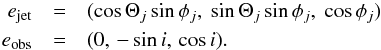 Here Θj is the jet azimuth (true anomaly), φj the jet polar angle (jet inclination=angle between the z-axis and the jet-axis) and i the orbital inclination (angle between the z-axis and the line-of-sight). The true anomaly is ± 90 deg at conjunctions (orbital phases 0 and 0.5). For the black hole case, Dubus et al. (2010) derived 39 deg and 319 deg for φj and Θj, respectively. Since the observer has a permanent 270 deg true anomaly (Θobs) and 30 deg inclination (φobs), the jet pointing is close to the line-of-sight. Hence, Cygnus X-3 is more likely a “microblazar” rather than a microquasar. Since the true jet anomaly is somewhat larger than that of the observer, the line-of-sight trails the jet during the orbit.
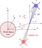 |
Fig. 1 System geometry (from Dubus et al. 2010). The jet-angles used are Θj = 319 deg and φj = 39 deg. The line of sight lies in a plane parallel to the yz-plane with direction Θ (=Θobs) = 270 deg and i (=φobs) = 30 deg. |
Besides the jet inclination and azimuth, an additional parameter in the modeling is the ratio H/d, where d is the binary separation and H the height along the jet where high energy electrons are released and Compton scattering takes place. Dubus et al. (2010) obtained a best value of 2.66 for this ratio. As an example, for total masses 12 M⊙ and 28 M⊙ the binary separation d is 3.2 R⊙ (2.2 × 1011 cm) and 4.2 R⊙ (4.2 × 1011 cm), respectively (the separation depends on total mass as Mtot1/3).
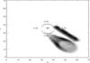 |
Fig. 2 Projection boundaries of bow shocks on the orbital xy-plane (pixel numbers marked) for the two geometries used at orbital phases 0.35 (the cone geometry) and 0.85 (the tube geometry). The WR-companion is in the center while the compact star is moving in a circular orbit around it (dotted circle). The observation direction is from below (see also Fig. 4). |
Numerical models for microquasar jets show a bow shock surrounding the jet (Perucho & Bosch-Ramon 2008). We used two simplified geometries to represent the stationary shocked region surrounding the jet: i) cone shells with thickness 0.1d and opening angles between 20–50 deg, and ii) cylinders with thickness 0.1d and radius between 0.2d–0.3d and starting at distances between 0–1.0d from the compact star. Further, we assume that the shocked region immediately transforms the wind material into clumps of equal density with space density Nwind/Nclump advected radially from the WR-star by velocities 1000–3000 km s-1. Nwind and Nclump are the wind and clump densities, respectively. Hence, the wind mass is conserved in the process. Note that this is just our assumption to explore the possibility of clumps without demonstrating that they really exist. In numerical computations we used the xyz-grid divided into 70 × 70 × 70 pixels with pixel size 0.18d, giving 12.6d for the box size.
The cone geometry with opening angles less than 20 deg or larger than 50 deg did not produce any orbital modulation (Sect. 3), nor thinner tubes in the tube geometry. The shell thickness has a minimal impact since we are not interested in the absolute values of mass columns, but only relative values along the orbit.
The geometries are shown schematically in Fig. 2 as projections on the orbital plane. The WR-companion is in the center while the compact star is moving in a circular orbit around it (dotted circle wit four phases marked). The observation direction is from below (see also Fig. 4). Note that the projections appear to end before reaching the grid boundaries (0, 70) due to small jet inclination (39 deg).
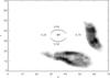 |
Fig. 3 Projections of the shocked regions in Fig. 2 (assumed to be transformed into clumps) and advected by the wind (2000 km s-1) during one hour (0.2 × orbital period). The WR-companion is in the center while the compact star is moving in a circular orbit around it (dotted circle). The observation direction is from below (see also Fig. 4). |
3. The “clumpy trail” and the two absorbers
We assume that the bow shock triggers the formation of dense clumps or makes the existing clumps in the WR wind denser. The formation of clumps migh physically similar to star formation when a shock front impinges upon interstellar clouds (van Breugel et al. 2004). Furthermore, we assume that these clumps participate in the wind outflow with velocity between 1000–3000 km s-1. Hence, once formed the clumps flow out with the wind. We stress that we just want to explore the possibility of clumps without demonstrating that they really exist.
We assume that the clump density (like the wind density) decreases with distance r from the WR-star as r− γ with γ = 2. The binary separation d = 3.4 R⊙ used in the computations obviously scales with the wind velocity.
An example of the initial jet bow shock from many computations is shown in Fig. 2 for a wind velocity 2000 km s-1, a cone with opening angle 20 deg (at orbital phase 0.35), and a tube with radius 0.3d (at orbital phase 0.85). We further assume that the bow shocks transform wind material immediately into dense clumps, to be advected by the wind. The projections of the advected clumps on the orbital plane are shown one hour later in Fig. 3. When coupling similar images over all phases and times we get the outflowing formation we call the “clumpy trail”. Thus the trail is the whole volume of clumps generated by the wind advection.
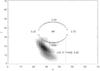 |
Fig. 4 Clump density along the crossing of the line-of-sight and clumpy trail (the strip), integrated over all phases and projected on the orbital xy-plane (for the cone in Fig. 2). The WR star is in the center, while the compact star is moving in a circular orbit around it (four orbital phases are shown). The projection of the line-of-sight at phase 0.65 is indicated by the vertical line. |
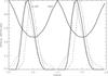 |
Fig. 5 The two absorbers τ(wind) and τ(clump) used in the modeling in Sect. 4 (solid lines) where τ(clump) corresponds in cone geometry to jet opening angle 20 deg and wind velocity 2000 km s-1. The dashed line has opening angle 20 deg and smaller 1000 km s-1 wind velocity. The two almost coincident dotted lines correspond to a wide cone (40 deg, 2000 km s-1) and a tube (see the text in Sect. 3). |
The crossing of the line-of-sight (from the compact star) and the clumpy trail was then computed numerically. For a fixed orbital phase this intersection is a segment (“strip”) of the line-of-sight along which the clump density is weighted by r-2. For the cone in Fig. 2 these strips integrated over all phases are shown in Fig. 4 as projected on the orbital plane (note the small inclination of 30 deg used and twice smaller pixel size used in this plot). The crossing region distance r from the compact star is between 0.3–3d (1–10 R⊙) at the ionization parameter range log (ξ) = 3.75−2.75 erg cm/s for density 1012 cm-3 (ξ = L/(Nr2)). In this plot we use a smaller pixel size than in Fig. 2 (0.09d) to better reveal the details.
Mass columns (assumed proportional to optical depths) along the line-of-sight for three cone models (20 deg, 1000 km s-1), (20 deg, 2000 km s-1), (40 deg, 2000 km s-1) and a tube with radius 0.3d are shown in Fig. 5, scaled with their maximum values along the orbit (dotted lines). The average phase at maxima is around 0.35 while the FWHM is approximately 0.25. The solid line is from the individual cone model in Figs. 2 and 3 (opening angle 20 deg, wind velocity 2000 km s-1). Amongst the dozen computed models, the latter produced the best fitting results and will be used as the clumpy trail absorber τ(clump) (see Sect. 4).
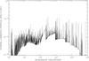 |
Fig. 6 Radiation spectrum of a clump (erg/s/keV per particle) with density N = 1013 cm-3 and in equilibrium temperature (around 105 K) at a distance of 3 R⊙ from the compact star (with Lx = 2.46 × 1038 erg/s). |
In the same plot (Fig. 5) we include the wind optical depth τ(wind) (=mass column along the line-of-sight, the solid line with maximum around phase 0). This will be used as the first absorber (wind absorber τ(wind)) in Sect. 4. Using (mass column)2 for the optical depth would give a better fit for the continuum light curve around minimum, and it may reflect that γ in reality is larger than 2 (accelerating wind) or else there is an ionization effect in the wind. Using a pure mass column yielded practically the same continuum light curve but with a partial eclipse profile that was slightly too broad.
Around φj = 39 deg the results are not very sensitive on this jet inclination angle, while changing Θj between 290 deg−340 deg moves the maximum of τ(clump) between 0.25–0.40 in phase.
The key factor in this concept is whether the clumps formed are radiative or not. In our case, the wind (including clumps) is photoionised and very radiative. Hence, the concept should work (from shocks to dense clumps).
3.1. Cooling times of shocked clumps
Bearing in mind that we have assumed, for the purpose of this paper, that a bow shock triggers clump formation, we nevertheless estimate cooling times for clumps, both in equilibrium with the radiation field as well as heated to 107 K. We speculate that hot clumps could exist at short distances from their origin and this is discussed in Sect. 5.
To estimate cooling times we use the photoionisation model of Vilhu et al. (2009), where the compact star luminosity is Lx = 2.46 × 1038 erg/s. The clump densities probably vary, as do their sizes, but as an example we use a density of 1013 cm-3. Based on our XSTAR-computations with inclination 30 deg, the wind base density should be around 1012 cm-3 to guarantee a continuum optical depth around unity (at 2 keV). This is what the partial eclipse of the continuum light curve requires (see Sect. 4). A somewhat higher clump density is then a good guess.
The radiation spectrum of a clump in equilibrium with density 1013 cm-3 at a distance of 3 R⊙ from the compact star (log (ξ) = 3.75) is shown in Fig. 6, as computed with the XSTAR code (Kallman 2006). In this model, the total outward luminosity Lout per clump particle equals 4.2 × 10⁻⁹ erg/s, while its thermal content per particle in equilibrium with the radiation field (temperature approximately 105 K) is 1.38 × 10⁻¹¹ erg.
Hence, the cooling time is short (3.3 ms) but this is counterbalanced by heating from the radiation field (heating = cooling in equilibrium). For a clump with N = 1012 cm-3 the cooling time is 20 ms (with similar equilibrium temperature 105 K). Cooling times for hot 107 K clumps (collision dominated) are almost 1000 times longer: 3 s and 17 s for densities 1013 cm-3 and 1012 cm-3, respectively. This is due to a heat content that is 100 times larger and outward luminosities 10 times smaller of the 107 K clumps. Cooling times of 108 K clumps can be several minutes.
Hot 107 K clumps are not in equilibrium with the surrounding radiation field and try to expand (and cool) after the shock has passed. A crude estimate of the dynamical time scale can be found as follows. The force F across the clump surface area S is P × S, where P is the gas pressure inside a clump with mass m. From the clump expansion acceleration a = F/m, one can compute that the dynamical expansion time is 3.5 s and 35 s for clump sizes 108 cm and 109 cm, respectively (independent of clump density).
Hence, hot 107 K clumps can survive at most a few minutes after their formation, depending on their density and size. Their possible role is discussed in Sect. 5.
4. Modeling of the X-ray continuum and emission line light curves
Here we compare the observed light curves with models using two absorbers: i) the WR wind; and ii) an absorber lying in the clumpy trail (see Fig. 4). Both optical depths are plotted in Fig. 5 and explained in Sect. 3.
The observed gamma-ray (Fermi/LAT) light curve is taken from Abdo et al. (2009) using the pdf measuring perimeter tool for graphics (Adobe) and modeled with Dubus et al. (2010) inverse Compton scattering formulas and parameters (i = 30 deg, φj = 39 deg, Θj = 319 deg, H/d = 2.66). The same parameter values were used for the clumpy trail computation. Note that Dubus et al. (2010) used phase units where the X-ray minimum occurs at phase 0.25. In this paper we use the X-ray phases where the X-ray minimun occurs at phase 0 (the WR star is between the observer and the compact star). For a jet with φj = i and Θj = 270 deg, the jet axis and line-of-sight would coincide.
The RXTE/ASM light curve integrated over fifteen years, and scaled inside a specific orbit by the daily mean, was used as a template for the continuum light curve. The ephemeris of Singh et al. (2002) was used to compute the orbits. The data were limited to moderately high states (daily means ≥ 15 counts/s), to be more consistent with the Cygnus X-3 spectral state during the Chandra/HETG observations used. The emission line light curves (Si XIV Lyα 6.185 Å, FeXXVI Lyα 1.780 Å (H-type) and FeXXV 1.859 Å (He-type)) were taken from Vilhu et al. (2009) and observed during a high state by Chandra/HETG (PI McCollough). The number of phase bins used was 30 and 10 for the continuum and lines, respectively.
The modeling of the light curves requires implementation of both the wind and clumpy trail absorbers explained in previous sections. We assume that the continuum soft X-ray emission is centered at the compact star (disc). Most line emission (in particular SiXIV) comes from a broad region in the wind, except the high excitation FeXXVI Lyα emission that probably originates from the compact star disc (see Vilhu et al. 2009). Line absorption in the continuum (at wavelengths below the line) should then be the common factor for all the lines.
Let τ(wind) and τ(clump) be the optical depths along the line-of-sight (from the compact star) in the wind and clumpy trail, respectively, and scaled with their maximum values along the orbit (as shown in Fig. 5). As baseline absorbers we adopt those delineated by the heavy solid lines in Fig. 5 and described in Sect. 3.
The model flux is defined with the help of these two absorbers as follows:
![Mathematical equation: $$ F = \exp[-A\tau({\rm wind}) - B\tau({\rm clump})] . $$](/articles/aa/full_html/2013/02/aa19843-12/aa19843-12-eq86.png) A and B are constants derived from the fitting to observations and given in Table 1 (using the baseline absorbers). The IDL procedure mpcurvefit.pro1 was used in the fitting. The F-statistic and the significance (between 0.0–1.0) of the fit was computed with the IDL-procedure fv − test.pro where 1.0 represents the highest significance. Table 1 shows that the fits are significant for both the continuum and the lines. If the clumpy trail absorber is not used at all (see Table 2) the fits are not acceptable, in particular for the lines.
A and B are constants derived from the fitting to observations and given in Table 1 (using the baseline absorbers). The IDL procedure mpcurvefit.pro1 was used in the fitting. The F-statistic and the significance (between 0.0–1.0) of the fit was computed with the IDL-procedure fv − test.pro where 1.0 represents the highest significance. Table 1 shows that the fits are significant for both the continuum and the lines. If the clumpy trail absorber is not used at all (see Table 2) the fits are not acceptable, in particular for the lines.
Figure 7 shows the observations overplotted with model fits. The mean light curve for the lines is shown, but note that Table 1 gives fitting parameters for all the lines. The contributing optical depths, Aτ(wind) and Bτ(clump), are also shown in the two lower plots by dotted lines (scaled with the continuum wind column Aτ(wind)). The scale on the left is the same as for the light curves. The gamma-ray (Fermi/LAT) light curve is shown for comparison in the uppermost panel.
It can be seen that most continuum modulation comes from the wind while the small asymmetry around phase 0.3–0.4 is caused by the clumpy trail (B much smaller than A, see Table 1). On the contrary, emission line absorption is enhanced at the clumpy trail (larger B).
Fitting parameters and significances for the ASM-continuum (daily means ≥ 15 cps) and Chandra emission line light curves.
Fitting parameters and significances for the pure wind absorber (τ(clump) = 0 or B = 0).
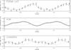 |
Fig. 7 Observed (crosses) and model (solid) light curves for gamma-ray (top, Fermi/LAT), X-ray continuum (middle, ASM daily mean ≥ 15 cps) and mean of SiXIV, FeXXV and FeXXVI emission lines (bottom, Chandra/HETG). The dotted lines in the two lowest panels show the contributing optical depths of the two absorbers (wind and clumpy trail), scaled with the maximum of continuum wind absorption (the same scale on the left as for the light curves). |
5. Discussion
The continuum light curve is represented by the ASM average light curve over fifteen years limited to daily means ≥ 15 counts/s. So far there is no clear evidence that the form of the light curve changes during this time nor depends on spectral state – low (hard) or high (soft) – in a significant way. However, we limited the ASM data to relatively high states to be more consistent with the emission line observations.
The emission line light curves were observed during a high state and with a few days’ exposure by Chandra/HETG (Vilhu et al. 2009, PI McCollough). It was assumed that they are representative also for the whole set of ASM observations. This is just an assumption and has no observational verification due to the limited amount of spectral data. The same applies for the Fermi/LAT gamma-ray observations since they are means over one year of observations during flaring periods (Dubus et al. 2010).
We assumed that the eventual jet precession has a long time scale (over tens of years). Otherwise the observations could not be compared with the same jet parameters. This appears to be the case, since most imaging radio observations between 1991 Jan. 15–2001 Sept. 15 locate the jet position angle in the North-South direction (0 deg or 180 deg; Martí et al. 2000, 2001; Miller-Jones et al. 2004; Schalinski et al. 1998). However, Tudose et al. (2007) using 2006 May 01 observations locate knots (which might be interpreted as segments of jets or counter jets) at position angles 55 deg–82 deg. Furthermore, Mioduszewski et al. (2001) locate the position angle during the 1997 Feb. 06 observations at 145 deg. We also assumed that the clumpy trail (in the circumbinary region) is more or less the same during all observations (including big flares or micro-flaring).
The physical nature of the two absorbers requires more work. At soft X-rays below 10 keV photoelectric absorption is important and depends both on the distance from the X-ray source and wind density. It also depends on the element and line transition in question. Pure electron scattering (depending on the number of particles along the line of sight) contributes in a small way. To illustrate the situation we computed three different scenarios with the XSTAR code (using the X-ray source model explained in Sect. 3.1) along the line-of-sight from the X-ray source at phase 0.35 (at the strip-segment 0.3d–3d from the source, see Fig. 4):
-
1.
Original wind – the wind was homogeneous with densitydecreasing as r-2 with distance r from the WR-star (1012 cm-3 at the WR-surface.
-
2.
Equilibrium clumps – the wind consisted of equilibrium clumps with density 1013 cm-3 (in equilibrium with the radiation field).
-
3.
107 K clumps – the clumps were forced to high constant temperature 107 K.
In all cases the mass columns along the line of sight strip were the same (wind mass conserved).
Continuum and line optical depths were computed along the strip using the XSTAR-code. Table 3 gives the integrated depths while Fig. 8 gives the optical depths per 1010 cm versus distance from th X-ray source (in units of the binary separation). In the plot the clumps are presented by a mixture (50/50) of equilibrium and 107 K clumps (solid lines). This mixture gives a moderate fit to the B-parameter values of Table 1, provided that the wind base density is twice larger 2 × 1012 cm-3. The pure wind case is shown by dashed lines. The dotted lines give the continuum for clumps (upper line) and wind (lower line) cases.
Table 3 and Fig. 8 show that the line absorption can indeed be enhaced at the clumpy trail. The iron lines appear to require hot collision dominated clumps (hotter than the equilibrium ones), in particular at short distances from the X-ray source. Replacing the clump density 1013 cm-3 by 1012 cm-3 or 1014 cm-3 does not change much this picture. The short cooling times (see Sect. 3.1) seem to require some modification to our assumptions: e.g. the jet axis is closer to the line of sight, the jet cone is broader, the bow shock propagates with the wind or clump formation is delayed.
Integrated optical depths along the “strip” (crossing of line-of-sight with the clumpy trail) at phase 0.35.
It is noteworthy that the presence of the clumpy trail absorber occurs around phase 0.3 (see Fig. 3) which is also where the 9 mHz QPOs were found by Koljonen et al. (2011). Whether these QPOs arise from some sort of flickering when the line of sight passes the moving clumps remains to be solved.
In the present paper a formal exponential law with two absorbers was used to model the light curves (Sect. 4). However, it is significant to note that the location of the second absorber coincides with the clumpy trail region.
6. Conclusions
We have demonstrated a possible method to study observable effects of jets in microquasars when the jet direction and line-of-sight are close to each other (as in Cygnus X-3). In particular, we showed that the jet in Cygnus X-3 can produce a “clumpy trail” which crosses the line-of-sight during the binary orbit periodically.
Using jet parameters derived by Dubus et al. (2010) from Fermi/LAT observations, we computed the location of the clumpy trail (see Fig. 3). Model light curves were then constructed using the two absorbers in Fig. 5 weighted with constants A and B: i) the WR wind; and ii) a clumpy trail. These light curves were compared with the observed ones. Good agreements were achieved for the soft X-ray continuum (RXTE/ASM) and emission lines (Chandra/HETG; see Fig. 7 and Table 1).
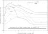 |
Fig. 8 Optical depths vs. distance from the X-ray source along the crossing of line-of-sight with the clumpy trail at phase 0.35 (see Fig. 4 and text in Sect. 5). |
We found that the location of the clumpy trail computed from jet parameters matches well with that of the second absorber required (clumpy trail absorber) which may not be just a coincidence. Although more work is required to clarify the physical nature of this clumpy absorber, we suggest that the clumpy trail consists of a mixture of equilibrium and hot (shock heated) clumps.
We note that the results are based on an assumption of constancy of the jet position angle over the past fifteen years (long precession time) which needs to be confirmed.
Written by Craig Markwardt.
Acknowledgments
We thank the referee for valuable criticism that greatly improved the paper. We are grateful to Dr. Guillaume Dubus for correspondence and permission to use his plot (Fig. 1). We also thank Wiley Publishers for permission to reproduce this figure. We thank Dr. Pasi Hakala for useful comments on the manuscript.
References
- Abdo, A. A., et al. (Fermi-LAT collaboration) 2009, Science, 326, 1512 [NASA ADS] [CrossRef] [PubMed] [Google Scholar]
- Crowther, P. A. 2007, ARA&A, 45, 177 [NASA ADS] [CrossRef] [Google Scholar]
- Dubus, G., Cerutti, B., & Henri, G. 2010, MNRAS, 404, L55 [NASA ADS] [Google Scholar]
- Hamann, W-R., Feldmeier, A., & Oskinova, L. M. 2008, in Clumping in Hot Star Winds, Proc. Int. Workshop held in Potsdam, Germany, 18–22 June 2007, Potsdam: Univ.-Verl. [Google Scholar]
- Hanson, M. M., Still, M. D., & Fender, R. P. 2000, ApJ, 541, 308 [NASA ADS] [CrossRef] [Google Scholar]
- Hjalmarsdotter, L., Zdziarski, A. A., Szostek, A., & Hannikainen, D. C. 2009, MNRAS, 392, 251 [NASA ADS] [CrossRef] [Google Scholar]
- Kallman, T. R. 2006, A Spectral Analysis Tool XSTAR, version 2.1kn6, Goddard Space Flight Center, May 25, 2006 [Google Scholar]
- Koljonen, K. I. I., Hannikainen, D. C., McCollough, M. L., Pooley, G. G., & Trushkin, S. A. 2010, MNRAS, 406, 307 [NASA ADS] [CrossRef] [Google Scholar]
- Koljonen, K. I. I., Hannikainen, D. C., & McCollough, M. L. 2011, MNRAS, 416, L84 [NASA ADS] [CrossRef] [Google Scholar]
- Langer, N. 1989, A&A, 210, 93 [NASA ADS] [Google Scholar]
- Liu, Q. Z., van Paradijs, J., & van den Heuvel, E. P. J. 2007, A&A, 469, 807 [NASA ADS] [CrossRef] [EDP Sciences] [Google Scholar]
- Martí, J., Paredes, J. M., & Peracaula, M. 2000, ApJ, 545, 939 [NASA ADS] [CrossRef] [Google Scholar]
- Martí, J., Paredes, J. M., & Peracaula, M. 2001, A&A, 375, 476 [NASA ADS] [CrossRef] [EDP Sciences] [Google Scholar]
- Miller-Jones, J. C. A., Blundell, K. M., Rupen, M. P., et al. 2004, ApJ, 600, 368 [NASA ADS] [CrossRef] [Google Scholar]
- Mioduszewski, A. J., Rupen, M. P., Hjellming, R. M., et al. 2001, ApJ, 553, 766 [NASA ADS] [CrossRef] [Google Scholar]
- Perucho, M., & Bosch-Ramon, V. 2008, A&A, 482, 917 [NASA ADS] [CrossRef] [EDP Sciences] [Google Scholar]
- Perucho, M., & Bosch-Ramon, V. 2012, A&A, 539, A57 [NASA ADS] [CrossRef] [EDP Sciences] [Google Scholar]
- Schalinski, C. J., Johnston, K. J., Witzel, A., et al. 1998, A&A, 329, 504 [NASA ADS] [Google Scholar]
- Szostek, A., & Zdziarski, A. A. 2008, MNRAS, 386, 593 [NASA ADS] [CrossRef] [Google Scholar]
- Singh, N. S., Naik, S., Paul, B., et al. 2002, A&A, 392, 161 [NASA ADS] [CrossRef] [EDP Sciences] [Google Scholar]
- Tudose, V., Fender, R. P., Garrett, M. A., et al. 2007, MNRAS, 375, L11 [NASA ADS] [CrossRef] [Google Scholar]
- van Breugel, W., Fragile, C., Anninos, P., & Murray S. 2004, Jet-induced star formation, IAU Symp. Ser., 217, 472 [Google Scholar]
- van Kerkwijk, M. H., Charles, P. A., Geballe, T. R., et al. 1992, Nature, 355, 703 [NASA ADS] [CrossRef] [Google Scholar]
- van Kerkwijk, M. H., Geballe, T. R., King, D. L., et al. 1996, A&A, 314, 521 [NASA ADS] [Google Scholar]
- Vilhu, O., Hakala, P., Hannikainen, D. C., McCollough, M., & Koljonen, K. 2009, A&A, 501, 679 [NASA ADS] [CrossRef] [EDP Sciences] [Google Scholar]
All Tables
Fitting parameters and significances for the ASM-continuum (daily means ≥ 15 cps) and Chandra emission line light curves.
Fitting parameters and significances for the pure wind absorber (τ(clump) = 0 or B = 0).
Integrated optical depths along the “strip” (crossing of line-of-sight with the clumpy trail) at phase 0.35.
All Figures
|
Fig. 1 System geometry (from Dubus et al. 2010). The jet-angles used are Θj = 319 deg and φj = 39 deg. The line of sight lies in a plane parallel to the yz-plane with direction Θ (=Θobs) = 270 deg and i (=φobs) = 30 deg. |
| In the text | |
|
Fig. 2 Projection boundaries of bow shocks on the orbital xy-plane (pixel numbers marked) for the two geometries used at orbital phases 0.35 (the cone geometry) and 0.85 (the tube geometry). The WR-companion is in the center while the compact star is moving in a circular orbit around it (dotted circle). The observation direction is from below (see also Fig. 4). |
| In the text | |
|
Fig. 3 Projections of the shocked regions in Fig. 2 (assumed to be transformed into clumps) and advected by the wind (2000 km s-1) during one hour (0.2 × orbital period). The WR-companion is in the center while the compact star is moving in a circular orbit around it (dotted circle). The observation direction is from below (see also Fig. 4). |
| In the text | |
|
Fig. 4 Clump density along the crossing of the line-of-sight and clumpy trail (the strip), integrated over all phases and projected on the orbital xy-plane (for the cone in Fig. 2). The WR star is in the center, while the compact star is moving in a circular orbit around it (four orbital phases are shown). The projection of the line-of-sight at phase 0.65 is indicated by the vertical line. |
| In the text | |
|
Fig. 5 The two absorbers τ(wind) and τ(clump) used in the modeling in Sect. 4 (solid lines) where τ(clump) corresponds in cone geometry to jet opening angle 20 deg and wind velocity 2000 km s-1. The dashed line has opening angle 20 deg and smaller 1000 km s-1 wind velocity. The two almost coincident dotted lines correspond to a wide cone (40 deg, 2000 km s-1) and a tube (see the text in Sect. 3). |
| In the text | |
|
Fig. 6 Radiation spectrum of a clump (erg/s/keV per particle) with density N = 1013 cm-3 and in equilibrium temperature (around 105 K) at a distance of 3 R⊙ from the compact star (with Lx = 2.46 × 1038 erg/s). |
| In the text | |
|
Fig. 7 Observed (crosses) and model (solid) light curves for gamma-ray (top, Fermi/LAT), X-ray continuum (middle, ASM daily mean ≥ 15 cps) and mean of SiXIV, FeXXV and FeXXVI emission lines (bottom, Chandra/HETG). The dotted lines in the two lowest panels show the contributing optical depths of the two absorbers (wind and clumpy trail), scaled with the maximum of continuum wind absorption (the same scale on the left as for the light curves). |
| In the text | |
|
Fig. 8 Optical depths vs. distance from the X-ray source along the crossing of line-of-sight with the clumpy trail at phase 0.35 (see Fig. 4 and text in Sect. 5). |
| In the text | |
Current usage metrics show cumulative count of Article Views (full-text article views including HTML views, PDF and ePub downloads, according to the available data) and Abstracts Views on Vision4Press platform.
Data correspond to usage on the plateform after 2015. The current usage metrics is available 48-96 hours after online publication and is updated daily on week days.
Initial download of the metrics may take a while.