| Issue |
A&A
Volume 550, February 2013
|
|
|---|---|---|
| Article Number | A35 | |
| Number of page(s) | 5 | |
| Section | Interstellar and circumstellar matter | |
| DOI | https://doi.org/10.1051/0004-6361/201219647 | |
| Published online | 22 January 2013 | |
Dust properties in the Galactic bulge⋆
1
Kapteyn Astronomical Institute,
PO Box 800,
9700 AV
Groningen,
The Netherlands
e-mail: This email address is being protected from spambots. You need JavaScript enabled to view it.
2
Institut d’Astrophysique Spatiale, Paris-Sud 11, 91405
Orsay,
France
Received: 22 May 2012
Accepted: 21 December 2012
Abstract
Context. It has been suggested that the ratio of total-to-selective extinction RV in dust in the interstellar medium differs in the Galactic bulge from its value in the local neighborhood.
Aims. We attempt to test this suggestion.
Methods. The mid-infrared hydrogen lines in 16 Galactic bulge PNe measured by the Spitzer Space Telescope are used to determine the extinction corrected Hβ flux. This is compared to the observed Hβ flux to obtain the total extinction at Hβ. The selective extinction is obtained from the observed Balmer decrement in these nebulae. The value of RV can then be found.
Results. The ratio of total-to-selective extinction in the Galactic bulge is consistent with the value RV = 3.1, which is the same as has been found in the local neighborhood.
Conclusions. The suggestion that RV is different in the Galactic bulge is incorrect. The reasons for this are discussed.
Key words: dust, extinction / planetary nebulae: general / infrared: ISM / radio continuum: ISM
Based on observations with the Spitzer Space Telescope, which is operated by the Jet Propulsion Laboratory, California Institute of Technology.
© ESO, 2013
1. Introduction
Interstellar extinction is a well studied but not completely understood phenomen. Beside studying the properties of the particles which cause the extinction, it is necessary to know the correction for extinction as a function of wavelength since individual measurements must be corrected for the effects of extinction.This has led to several Galactic extinction curves; the most commonly used are those of Savage & Mathis (1979), Seaton (1979) and Cardelli et al. (1988). These curves extend over the complete wavelength range through the ultraviolet to about 1000 Å. All three curves cited are quite similar and are generally used as an average Galactic extinction curve to correct observed spectra for the effects of extinction. While uncertainties exist in these curves in the ultraviolet part of the spectrum, the uncertainties in the visible and infrared regions are small, almost certainly less than 5% (e.g. Fitzpatrick 1999). An additional extinction curve has been proposed for the near and mid-infrared spectral region by Chiar & Tielens (2006).
Hβ values predicted by infrared hydrogen line and consequent values of Cir.
In the specific case of correcting the spectra of planetary nebulae for the effects of extinction two methods are used, both of which are based on the average Galactic extinction curve. The first makes use of a comparison of the observed Balmer decrement with that expected from optically thin nebulae using the theoretical values given by Hummer & Storey (1987). Ususally fitting the Hα/Hβ ratio is given the most weight. The best fit between the observed and theoretical Balmer decrement is usually given by the parameter Cbd which is the log of the value by which the observed Hβ must be increased to correct it for interstellar extinction. Cbd is a weak function of Te, the electron temperature, and RV, the ratio of total- to-selective extinction at visual wavelengths. A value of RV = 3.1 is usually used. In principle Cbd is also a function of the electron density, but it is such a weak function for the densities found in planetary nebulae that we will ignore it here.
The second method for correcting for the effects of extinction is to use the observed radio continuum emission. The radio emission is dependent on the product of the density of ionized hydrogen and the electron density in the same way as the Hβ emission is, so that the ratio is essentially density independent. The value of unreddened Hβ thus obtained may be used to compute Crad, similar to the value of C computed above but now derived from the radio continuum flux density. Note that Crad is a weak function of Te. It also depends on the abundance of (doubly) ionized helium which contributes to the electron density. But Crad is independent of RV. Note that it is also assumed that the nebula is optically thin to the radio emission so that all emission produced is measured. Because the geometry of the nebula is not known, the optical depth cannot be accurately computed. Because it is inversely proportional to the square of the frequency, the radio measurements should be made at the highest possible frequency.
Since Cbd and Crad are by definition equal and only Cbd depends on RV, information concerning this quantity can now be found if the Balmer decrement, the radio continuum flux density, the electron temperature and the amount of helium and its ionization are known. This method has already been applied to PNe in the Galactic bulge 20 years ago by Tylenda et al. (1992) and Stasinska et al. (1992). In the first of these articles the authors found that there was fair agreement between Cbd and Crad for small values of extinction, but for large extinctions Crad is smaller than Cbd. In the first paper they explain the difference as due to underestimates of the radio emission. In the second article they express more confidence in the radio measurements and now explain the difference as being due to a lower value of RV for the more distant nebulae. While these authors do not specifically refer to the Galactic bulge, about 30% to 40% of the PNe they use are Galactic bulge objects. Other authors (e.g. Hultzsch et al. 2007; and Ruffle et al. 2004) use this as evidence for a possibly lower value for RV in the Galactic bulge.
The calculation of Cbd and Crad is uncertain as these authors admit. First of all the electron temperature of the individual nebulae is unknown, so that a value of 10 000 K was always used. Secondly the helium abundance is unknown so that a 10% helium abundance is assumed, all in singly ionized form. Thirdly, the measurements of the Balmer decrement are sometimes of uncertain quality; in the few cases where multiple observations of a single object have been made conflicting results are sometimes obtained. Finally no correction has been attempted for possible optical depth effects in the 6 cm radio continuum except that objects with possibly high brightness temperature were removed from the sample. This method is not very reliable, as the above authors remark, because the surface brightness of PNe “is usually far from uniform and the estimate of the brightness temperature is very sensitive to the adopted nebular diameter”. The sample used by Stasinska et al. (1992) contained somewhat less than 199 Galactic bulge PNe, while the sample used by Ruffle et al. (2004) contained 12 Galactic bulge PNe. This latter sample, which reached the same conclusion as that of Stasinska et al. (1992), contains the same uncertain approximations.
There is a better method for comparing the Balmer decrement extinction with that determined from the total Hβ extinction. In this method the hydrogen lines in the mid-infrared are measured; in this part of the spectrum the interstellar extinction is very small. The intrinsic Hβ intensity is then derived from the mid-infrared line intensiy by the theoretical relations of Hummer & Storey (1987). To measure the mid-infrared lines we use the spectrograph on board the Spitzer Space Telescope which measures several hydrogen lines, the strongest being the H(6-5) transition at 7.46 μm (Paschen α) and, with a higher spectral resolution, the H(7-6) transition at 12.37 μm. The log of this predicted value of Hβ intensity divided by the observed Hβ intensity is called Cir and may be directly compared with Cbd to determine RV. In this way the radio continuum measurements are replaced by the infrared hydrogen line measurements; the radio measurements are no longer necessary to determine RV.
In Sect. 2 the infrared observations are presented and discussed, resulting in the determination of Cir. In Sect. 3 the Balmer decrement is discussed resulting in a value of Cbd. A comparison of these two values is made in Sect. 4, which leads to a conclusion about RV. At the same time Crad is computed and discussed.
Values of Cbd derived from the Balmer decrement.
2. The infrared spectrum
2.1. Observations
We have selected 16 planetary nebulae for measurement, which are almost certainly in the Galactic bulge. They are all within 10° of the Galactic center, they have low intrinsic radio continuum flux density and all but one have very high velocity with respect to the sun. The observations were made using the Infrared Spectrograph (IRS, Houck et al. 2004) on board the Spitzer Space Telescope with AOR keys both on target and on the background. The reduction of the spectra reported by Gutenkunst et al. (2007, see listing below) started from the droop images and is discussed in detail in that paper. The results given by Gutenkunst et al. (2007) are shown in Table 1. For the remaining extractions droop images are replaced by optimal extractions. The details of this reduction procedure are given in Pottasch & Bernard-Salas (in prep.).
Two of the three diaphragms used have high resolution: the short high module (SH) measures from 9.9 μm to 19.6 μm and the long high module (LH) from 18.7 μm to 37.2 μm. The SH has a diaphragm size of 4.7′′ × 11.3′′, while the LH is 11.1′′ × 22.3′′. The diameters of the PNe being measured are shown in Table 1. These are taken from a variety of sources, the most reliable are those of Sahai et al. (2011). For the other PNe the VLA radio continuum half width measurements listed by Acker et al. (1992) are given. The diameters are always considerably smaller than the LH diaphragm but may not always be smaller than the SH diaphragm. To correct for possible missing intensity in the SH diaphragm we examine the continuum intensity of LH and SH in the region of wavelength overlap at 19 μm. These continua should be equal if the entire nebula is being measured in the SH diaphragm. If this is not so all intensities in the SH diaphragm are increased by a factor which make the continua equal. The corrections are small for these nebulae, ususally between 1.1 and 1.3.
The third diaphragm is a long slit which is 4′′ wide and extends over the entire nebula. This SL module measures in low resolution between 5.5 μm and 14 μm. These spectra are normalized by making the strong lines in common between the SL and SH modules agree. Especially important is the agreement of the [S iv] line at 10.51 μm and the [Ne ii] line at 12.82 μm. Because all of the PNe measured are small, the corrections are likewise small. The resultant spectra may now be plotted. We have not done this here because good plots are already in the literature. Plots of He2-250, H2-11, He2-262, H1-15, H2-20, M2-31, M2-5, M2-10 and H1-20 may be found in Gutenkunst et al. (2007); plots of He2-260, M1-27, H1-43 and M3-44 can be found in Perea-Calderon et al. (2009); plots of M1-38 and M1-37 are found in Stanghellini et al. (2012). The excellent quality of the emission lines is apparent on the spectra.
The intensities of the 12.37 μm line (SH diaphragm) and the 7.46 μm line (SL diaphragm) are then be measured using the Gaussian line-fitting routine. The resultant values are shown in Cols. 3 and 4 of Table 1. The 3σ errors of measurement are always less than 20%. The 12.37 μm line has the more accurate intensity of the two lines in spite of the fact that it is intrinsically the weaker line. There are several reasons for this. First of all the 12.37 μm line is measured with a much higher resolution (about 600) compared to the 7.46 μm line (about 90). Secondly the measurement of the 7.46 μm line is difficult because it falls in the middle of overlapping orders. Thirdly the 12.37 μm line is often measured both at high resolution (SH) and at low resoluton (SL) and very similar intensities are found. For these reasons we give the value of the intrinsic Hβ found from the 12.37 μm line considerably more weight.
The Hβ flux is found from the infrared hydrogen lines using the theoretical ratios of Hummer & Storey (1987). It must be remembered that the 12.37 μm line is a blend of the H(7-6) transition with the H(11-8) line, while the 7.46 μm line is a blend of H(6-5) with H(8-6) and H(17-8). These blend are subtracted when deriving Hβ. Futhermore the ratios of the various hydrogen lines are weakly dependent on the electron temperature. The values of Te used are given in Col. 5 of Table 1 and are taken from Pottasch & Bernard-Salas (in prep.). The values of Hβ thus found are given in Cols. 6 and 7 of the table, derived respectively from the 7.46 μm line and from the 12.37 μm line. A small correction has been made for extinction at these wavelengths using the coefficients listed in Chiar & Tielens (2006). Because the extinction coefficients are small at these wavelengths, the corrections are insensitive to the precise value. For example, an extinction EB − V = 2 at 12.37 μm yields a correction of 10%. Thus any uncertainty in the mid infrared extinction is unimportant. Comparing Cols. 6 and 7, it can be seen that very similar values of Hβ are usually found from each of the lines. The combined value, given in Col. 8, is heavily weighted in favor of the value of Hβ found from the better measured 12.37 μm line. The observed value of Hβ is listed in Col. 9 and is usually taken from Acker et al. (1992). The difference between Cols. 9 and 8 is the value Cir given in the last column.
The 16 PNe listed in Table 1 were selected as Galactic bulge objects using three criteria. First and perhaps most important, is the high radial velocity of these PNe. Only png356.5-2.3 has a low velocity. This value is shown in the second column of the table. Secondly the diameter of the nebulae (listed in Table 2) is always less than 7′′. Thirdly, to insure that no nearby PNe are included, the 6 cm radio continuum flux density (listed in Table 3) is always less than 70 mJy. In addition it was important that additional information concerning the visible spectrum and continuum radio flux density be available. It may be noticed that the intrinsic Hβ flux of these nebulae (Col. 8 of Table 1) is always very similar; in all cases it is within a factor of 2 of a value −log Hβ = 11. The mass of each PN, computed for the case of a uniform constant density nebula, is also shown in Table 2. They are consistent with the nebulae being located in the Galactic bulge. Nine of these nebulae have been studied by Gutenkunst et al. (2007). We did not use the two further PNe studied by this group because no visual spectra are available. Four PNe are from a program to observe low excitation nebulae. The remaining three PNe (png2.4-3.7, 2.6-3.4 and 8.2+6.8) were inspired by the work of Hultzsch et al. (2007). The other two bulge PNe studied by these latter authors were not measured by the Spitzer Space Telescope.
2.2. The Balmer decrement and extinction
Selective extinction can be derived from the Balmer decrement assuming that the hydrogen lines are formed in an optically thin medium and their intrinsic ratios are given by the theory of Hummer & Storey (1987). Because measurements of the weaker Balmer lines are more uncertain for the bulge PNe more weight is usually given to the Hα/Hβ ratio; sometimes only this ratio is used. The value of total extinction at Hβ, Cbd, derived from this ratio may be written as: ![Mathematical equation: \begin{equation} C_{\rm bd}= X \log [I({\rm H}\alpha)/2.85I({\rm H}\beta)] \end{equation}](/articles/aa/full_html/2013/02/aa19647-12/aa19647-12-eq23.png) (1)where 2.85 is the intrinsic value of the ratio Hα/Hβ and is slightly dependent on the electron temperature. I(Hα)/I(Hβ) is the measured value of this ratio, while
(1)where 2.85 is the intrinsic value of the ratio Hα/Hβ and is slightly dependent on the electron temperature. I(Hα)/I(Hβ) is the measured value of this ratio, while  and A is the extinction in magnitudes at the wavelength given. These values depend on RV, the ratio of total to selective extinction. We use the value RV = 3.1 in the remainder of this section. Even having fixed the value of RV there is still a small uncertainty in the value of X to be used. Cardelli et al. (1988) find X = 3.36, Seaton (1979) derives a value of X = 3.23 from measurements of hydrogen and helium lines in NGC 7027 (he gives 3.17 as the expected standard value) and Savage & Mathis (1979) find X = 3.17. We assume that these values are all within the uncertainty of the determination and use in the following the slightly uncertain average value X = 3.17.
In Table 2 the values of Cbd found in the literature are given. Columns 4 and 5 are the values found using the Hα/Hβ ratio listed by Acker et al. (1992) and Escudero et al. (2004) in conjunction with Eq. (1). Columns (6) through (10) give the value of Cbd that the authors listed have derived from their spectra. Most authors do not give their measured spectral intensities but only the intensities after correction for extinction. Thus the precise extinction correction each individual author used cannot be found. This adds to the uncertainty. Comparing the different values of Cbd for a single object, we can obtain a feeling as to the accuracy of the individual values, which sometimes agree well with one another and sometimes show important differences. In the last column the average value of the measures for each PN are given.
Values of Crad derived from the 6 cm radio continuum.
2.3. Comparison of Cbd and Cir
Figure 1 is a plot of Cbd, taken from Table 2, against Cir, taken from Table 1. Approximate error bars are shown although the errors are rather difficult to specify accurately. The error in Cbd is determined by the consistency of the various values in individual objects where several measurements have been made. When only one or two measurements are available it is assumed that the uncertainty is similar to that of the better observed object. The uncertainty in Cir, which has been discussed above, is considerably smaller because the 12.37 μm line can be well measured. In addition, the uncertainty introduced by a diaphragm correction is probably not large (≤10%). On the whole one may say that there is good agreement between Cbd, found using a value of RV = 3.1, and Cir which does not depend on RV. Thus this value of RV is consistent for these Galactic bulge nebulae. This consistency removes the basis for the suggestion of Stasinska et al. (1992) that the value of the ratio of the total-to-selective extinction RV differs in the material closer to the Galactic center from the material farther out.
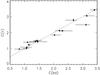 |
Fig. 1 Total extinction coefficient at Hβ derived from the far infrared hydrogen lines, Cir, is plotted as a function of the selective extinction coefficient at Hβ derived from the Balmer decrement, Cbd. The dashed line shows when these two quantities are equal. The error bars are discussed in the text. |
2.4. The 6 cm radio emission and Crad
Since the flux of the mid-infrared hydrogen lines were not yet known at the time of the work of Stasinska et al. (1992), these authors used the PNe radio continuum flux density to determine the intrinsic Hβ flux. As discussed earlier, in order to compute this intrinsic flux, one must know the electron temperature Te as well as the amount of He+ and He++, which are also responsible for the continuous radio emission. Furthermore the nebula must be optically thin to the radio radiation. The electron temperature (taken from an as yet unpublished study of Pottasch & Bernard-Salas) is listed in Table 1 as well as well as the ionized helium abundances in Cols. 2 and 3 of Table 3. The 6 cm flux density is listed in Col. 4 of Table 4; it has been measured mainly by Gathier et al. (1983), and also by Zijlstra et al. (1989), Pottasch et al. (1988) and Aaquist & Kwok (1990). The only nebula with an uncertain radio flux density is H2-20 which was only measured at 3 cm by Purton et al. (1982). It has a large error. The 6 cm flux density of this PN is discussed by Cahn et al. (1992), whose (uncertain) value is listed in Table 3. He2-367 is not on the list since no measurements of its radio continuum flus density have been made.
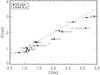 |
Fig. 2 Total extinction coefficient at Hβ derived from the 6 cm radio continuum flux density, Crad, is plotted as a function of the selective extinction coefficient at Hβ derived from the Balmer decrement, Cbd. The dashed line shows when these two quantities are equal. In addition to the PNe discussed in this paper, those discussed by Ruffle et al. (2004) are also plotted to demonstrate that these PNe lead to the same result. |
The resultant Hβ flux is listed in Col. 6 of Table 3 and the resultant Hβ extinction, Crad in Col. 7. These values of extinction have been plotted against the Balmer decrement extinction Cbd as Fig. 2. Comparing this figure with Fig. 1 shows that the points are on average somewhat to the right of the line of equal extinctions, i.e. the extinction derived from the radio flux density is somewhat lower than that indicated by the Balmer decrement. It is unlikely that this can be due to the use of an incorrect value of RV because it has already been established in the previous section that RV must be close to a value of 3.1. The problem must lie in the value of the 6 cm radio flux density. While it is possible that these measurements are incorrect, this is not likely because the errors would all have to be in the direction as to make the flux smaller than the actual value. It is more likely that the assumption that the nebulae are optically thin is not entirely correct because some absorption would make the fluxes of all PNe smaller. The following evidence supports this assumption. When the nebula is optically thin up to a wavelength of 21 cm, the 21 cm continuum flux density will be approximately a factor of 1.14 higher than the 6 cm flux density. To check this, Col. 5 of Table 3 lists the 21 cm flux density of these PNe, taken from the VLA measurements of Condon & Kaplan (1998). As can be seen, in only 5 of the 15 nebulae is the radio emission higher at 21 cm than at 6 cm. Thus optical depth effects are playing a role in this radio spectrum. Not enough information is available to quantify this effect for the individual nebulae, because very little is known about the distribution of matter in these PNe. The effect will always work in the direction of decreasing the predicted Hβ intensity and thus increasing Crad. This can be settled by obtaining radio measurements at a higher frequency.
In Fig. 2 the Galactic bulge PNe used by Ruffle et al. (2004) have also been plotted (open circles). Unfortunately less information is known for these nebulae (the electron temperature and the helium ionic abundances are unknown) and the only information about the Balmer decrement is that in the catalog of Acker et al. (1992), so that the average values used by Ruffle et al. (2004) were used and the extinction was obtained from the Balmer decrement as in Sect. 2.2. There is thus a somewhat greater uncertainty in these values. However, as can be seen from the figure there is no difference between the results from our PNe and those of Ruffle et al. (2004).
3. Conclusions
The Hβ flux has been derived from the mid-infrared hydrogen lines observed by the Spitzer Space Telescope for 16 planetary
nebulae in the Galactic bulge. These transitions, H(7-6) at 12.37 μm and H(6-5) at 7.45 μm, being relatively unaffected by Galactic extinction, make it possible to obtain the total extinction at Hβ. We emphasize that this is the most reliable method of obtaining the extinction and therefore Cir is more reliable than Crad. By combining Cir with the selective extinction obtained from measurements of the Balmer decrement for these same PNe, the value of the total-to-selective extinction, RV, can be approximately determined. The value found is consistent with RV = 3.1 which is the value of total-to-selective extinction ususally found in the interstellar material closer to the Sun.
This result is at odds with that of Stasinska et al. (1992) and of Ruffle et al. (2004). These authors obtained the total extinction by using the 6 cm radio continuum to determine the extinction-corrected Hβ flux. We discuss the reasons for this difference, which most likely is largly due to the assumption that the PNe are entirely optically thin at this 6 cm radio frequency.
Acknowledgments
We acknowledge the use of SIMBAD and ADS in this research work. J.B.-S. wishes to acknowledge the support from a Marie Curie Intra-European Fellowship within the 7th European Community Framework Program under project number 272820.
References
- Aaquist, O. B., & Kwok, S. 1990, A&AS, 84, 229 [NASA ADS] [Google Scholar]
- Acker, A., Marcout, J., Ochsenbein, F., et al. 1992, Strasbourg-ESO catalogue [Google Scholar]
- Bernard Salas, J., Pottasch, S. R., Beintema, D. A., & Wesselius, P. R. 2001, A&A, 367, 949 [NASA ADS] [CrossRef] [EDP Sciences] [Google Scholar]
- Cahn, J. H., Kaler, J. B., & Stanghellini, L. 1992, A&AS, 94, 399 [NASA ADS] [Google Scholar]
- Cardelli, J. A., Clayton, G. C., & Mathis, J. S. 1988, ApJ, 329, L33 [NASA ADS] [CrossRef] [Google Scholar]
- Ciardullo, R., Bond, H. E., & Sipior, M. S. 1999, AJ, 118, 488 [NASA ADS] [CrossRef] [Google Scholar]
- Chiar, J. E., & Tielens, A. G. G. M. 2006, ApJ, 637, 774 [NASA ADS] [CrossRef] [Google Scholar]
- Condon, J. J., & Kaplan, D. L. 1998, ApJS, 117, 361 [NASA ADS] [CrossRef] [Google Scholar]
- Cuisinier, F., Maciel, W. J., Koppen, J., et al. 2000, A&A, 353, 543 [NASA ADS] [Google Scholar]
- Escudero, A. V., Costa, R. D. D., & Maciel, W. J. 2004, A&A, 414, 211 [NASA ADS] [CrossRef] [EDP Sciences] [Google Scholar]
- Exter, K. M., Barlow, M. J., & Walton, N. A. 2004, MNRAS, 349, 1291 [NASA ADS] [CrossRef] [Google Scholar]
- Fitzpatrick, E. L. 1999, PASP, 111, 63 [NASA ADS] [CrossRef] [Google Scholar]
- Fluks, M. A., Plez, B., de Winter, D., et al. 1994, A&AS, 105, 311 [NASA ADS] [Google Scholar]
- Gathier, R., Pottasch, S. R., Goss, W. M., et al. 1983, A&A, 128, 325 [NASA ADS] [Google Scholar]
- Gorny, S. K., Chiappini, C., Stasinska, G., et al. 2009, A&A, 500, 1089 [NASA ADS] [CrossRef] [EDP Sciences] [Google Scholar]
- Gorny, S. K., Perea-Calderon, J. V., Garcia-Hernandez, D. A., et al. 2010, A&A, 516, A39 [NASA ADS] [CrossRef] [EDP Sciences] [Google Scholar]
- Gutenkunst, S., Bernard-Salas, J., Pottasch, S. R., et al. 2008, ApJ, 660, 1206 [NASA ADS] [CrossRef] [Google Scholar]
- Higdon, S. J. U., Devost, D., Higdon, J. L., et al. 2004, PASP, 116, 975 [NASA ADS] [CrossRef] [Google Scholar]
- Houck, J. R., Appleton, P. N., Armus, L., et. al. 2004, ApJS, 154, 18 [NASA ADS] [CrossRef] [Google Scholar]
- Hultzsch, P. J. N., Puls, J., Mendez, R. H., et al. 2007, A&A, 467, 1253 [NASA ADS] [CrossRef] [EDP Sciences] [Google Scholar]
- Hummer, D. G., & Storey, P. J. 1987, MNRAS, 224, 801 [NASA ADS] [CrossRef] [Google Scholar]
- Milne, D. K., & Aller, L. H. 1975, A&A, 38, 183 [NASA ADS] [Google Scholar]
- Milne, D. K., & Aller, L. H. 1982, A&AS, 50, 209 [NASA ADS] [Google Scholar]
- Perea-Calderon, J. V., Garcia-Hernandez, D. A., Garcia-Lario, P., et al. 2009, A&A, 495, L5 [NASA ADS] [CrossRef] [EDP Sciences] [Google Scholar]
- Pottasch, S. R., Bignell, C., Olling, R., et al. 1988, A&A, 221, 123 [Google Scholar]
- Pottasch, S. R., Bernard-Salas, J. 2010, A&A, 517, A95 [NASA ADS] [CrossRef] [EDP Sciences] [Google Scholar]
- Purton, C. R., Feldman, P. A., Marsh, K. A., et al. 1982, MNRAS, 198, 321 [NASA ADS] [CrossRef] [Google Scholar]
- Ratag, M. A. 1990, Thesis, Univ. Groningen [Google Scholar]
- Ruffle, P. M. E., Zijlstra, A. A., Walsh, J. R., et al. 2004, MNRAS, 353, 796 [NASA ADS] [CrossRef] [Google Scholar]
- Sahai, R., Morris, M. R., & Villar, G. G. 2011, AJ, 141, 134 [NASA ADS] [CrossRef] [Google Scholar]
- Savage, B. D., & Mathis, J. S. 1979, ARA&A, 17, 73 [NASA ADS] [CrossRef] [Google Scholar]
- Seaton, M. J. 1979, MNRAS, 187, 73 [Google Scholar]
- Stanghellini, L., Garcia-Hernandez, D. A., Garcia-Lario, P., et al. 2012, ApJ, 753, 172 [NASA ADS] [CrossRef] [Google Scholar]
- Stasinska, G., Tylenda, R., Acker, A., et al. 1992, A&A, 266, 486 [NASA ADS] [Google Scholar]
- Surendiranath, R., Pottasch, S. R., & García-Lario, P. 2004, A&A, 421, 1051 [NASA ADS] [CrossRef] [EDP Sciences] [Google Scholar]
- Tylenda, R., Acker, A., Stenholm, B., et al. 1992, A&AS, 95, 337 [NASA ADS] [Google Scholar]
- Wang, W., & Liu, X.-W. 2007, MNRAS, 381, 669 [NASA ADS] [CrossRef] [Google Scholar]
- Zijlstra, A. A., Pottasch, S., & Bignell, C. 1989, A&AS, 79, 329 [NASA ADS] [Google Scholar]
All Tables
All Figures
|
Fig. 1 Total extinction coefficient at Hβ derived from the far infrared hydrogen lines, Cir, is plotted as a function of the selective extinction coefficient at Hβ derived from the Balmer decrement, Cbd. The dashed line shows when these two quantities are equal. The error bars are discussed in the text. |
| In the text | |
|
Fig. 2 Total extinction coefficient at Hβ derived from the 6 cm radio continuum flux density, Crad, is plotted as a function of the selective extinction coefficient at Hβ derived from the Balmer decrement, Cbd. The dashed line shows when these two quantities are equal. In addition to the PNe discussed in this paper, those discussed by Ruffle et al. (2004) are also plotted to demonstrate that these PNe lead to the same result. |
| In the text | |
Current usage metrics show cumulative count of Article Views (full-text article views including HTML views, PDF and ePub downloads, according to the available data) and Abstracts Views on Vision4Press platform.
Data correspond to usage on the plateform after 2015. The current usage metrics is available 48-96 hours after online publication and is updated daily on week days.
Initial download of the metrics may take a while.