| Issue |
A&A
Volume 550, February 2013
|
|
|---|---|---|
| Article Number | A92 | |
| Number of page(s) | 19 | |
| Section | Cosmology (including clusters of galaxies) | |
| DOI | https://doi.org/10.1051/0004-6361/201117376 | |
| Published online | 31 January 2013 | |
A multi-frequency study of the SZE in giant radio galaxies
1 INAF – Osservatorio Astronomico di Roma via Frascati 33, 00040 Monteporzio, Italy
e-mail: This email address is being protected from spambots. You need JavaScript enabled to view it.
2 University of the Witwatersrand, Johannesburg, Private Bag 3, 2054 Gauteng, South Africa
e-mail: This email address is being protected from spambots. You need JavaScript enabled to view it.
3 Dipartimento di Fisica, Università di Roma La Sapienza, P. le A. Moro 2, Roma, Italy
Received: 30 May 2011
Accepted: 27 September 2012
Abstract
Context. Radio galaxy (RG) lobes contain relativistic electrons embedded in a tangled magnetic field that produce, in addition to low-frequency synchrotron radio emission, inverse-Compton scattering (ICS) of the cosmic microwave background (CMB) photons. This produces a relativistic, non-thermal Sunyaev-Zel’dovich effect (SZE).
Aims. We study the spectral and spatial properties of the non-thermal SZE in a sample of radio galaxies and make predictions for their detectability in both the negative and the positive part of the SZE, with space experiments like Planck, OLIMPO, and Herschel-SPIRE. These cover a wide range of frequencies, from radio to sub-mm.
Methods. We model the SZE in a general formalism that is equivalent to the relativistic covariant one and describe the electron population contained in the lobes of the radio galaxies with parameters derived from their radio observations, namely, flux, spectral index, and spatial extension. We further constrain the electron spectrum and the magnetic field of the RG lobes using X-ray, gamma-ray, and microwave archival observations.
Results. We determine the main spectral features of the SZE in RG lobes, namely, the minimum, the crossover, and the maximum of the SZE. We show that these typical spectral features fall in the frequency ranges probed by the available space experiments. We provide the most reliable predictions for the amplitude and spectral shape of the SZE in a sample of selected RGs with extended lobes. In three of these objects, we also derive an estimate of the magnetic field in the lobe at the ~μG level by combining radio (synchrotron) observations and X-ray (ICS) observations. These data, together with the WMAP upper limits, set constraints on the minimum momentum of the electrons residing in the RG lobes and allow realistic predictions for the visibility of their SZE to be derived with Planck, OLIMPO, and Herschel-SPIRE.
Conclusions. We show that the SZE from several RG lobes can be observed with mm and sub-mm experiments like Planck, OLIMPO, and Herschel-SPIRE, as well as with ground-based telescopes that have ≲ mJy sensitivity and sub-arcmin spatial resolution. These measurements will be crucial to disentangle the relativistic electron distribution from that of the magnetic field in RG lobes and to constrain the properties of their ICS emission, which is also visible at very high X-ray and gamma-ray energies.
Key words: cosmology: theory / cosmic background radiation / galaxies: active
© ESO, 2013
1. Introduction
The lobes of giant radio galaxies are unique laboratories for constraining the plasma processes that accelerate and diffuse relativistic electrons within large intergalactic volumes. Studies of radio galaxy (RG) lobes (e.g., Harris & Krawczynski 2002; Kataoka et al. 2003; Kronberg et al. 2004; Croston et al. 2005; Blundell et al. 2006, and references therein) have shown, in fact, that these extended structures contain relativistic electrons embedded in a tangled magnetic field that produce both low-frequency synchrotron radio emission and inverse-Compton scattering (ICS) of cosmic microwave background (CMB) photons, a mechanism hereafter referred to as ICCMB, as well as other radiation background.
Synchrotron radio emission and polarization are ubiquitously observed in all the extended lobes of radio galaxies and testify to the presence of a plasma of relativistic particles embedded in a tangled magnetic field. Radio emission polarization and Faraday Rotation measures also provide detailed information on the structure of the magnetic field in and around the RG lobes (see, e.g., Guidetti et al. 2011, and references therein). These observations show, for instance, a typical amplitude B0 ≈ 1.8 μG of the central B-field in the lobes of the RG 0208+35, assuming a typical variation of the field strength with radius in the intracluster atmosphere around the RG.
The ICCMB mechanism up-scatters the CMB photons over a wide range of frequencies, allowing the detection of such emission even at high energies, where it can be observable in X-rays and gamma-rays. Extended X-ray emission has been, in fact, observed by Chandra in the lobes of several powerful radio galaxies (see, e.g., the cases of 3C 432, 3C 294 and 3C 191 discussed by Erlund et al. 2006) and is due to ICCMB photons by the relativistic electrons confined in the RG lobes. This is consistent with previous findings of X-ray emission from the lobes of FR-II radio galaxies (like 3C 223 and 3C 284, see Croston et al. 2004) attributed to the same ICCMB mechanism. The Fermi-LAT gamma-ray detection of a spatially resolved gamma-ray glow emanating from the giant radio lobes of Centaurus A (Abdo et al. 2010) also indicates that the radio-lobe gamma-ray emission is mainly due to ICCMB, with the additional contribution, at higher energies, from the infrared-to-optical extragalactic background light.
As a consequence of the pervading presence of the ICCMB mechanism in extended RG lobes, a Sunyaev-Zel’dovich effect (SZE) from the lobes of radio galaxies is inevitably expected (Colafrancesco 2008). Such a non-thermal, relativistic SZE has a specific spectral shape that depends on the shape and on energy extent of the spectrum of the electrons residing in the RG lobes.
The SZE from RG lobes has a wide astrophysical and cosmological relevance, which allows the study of, e.g., the energetics and pressure structure of the RG lobes, the detailed structure of their B-field in combination with radio synchrotron observations, and the evolution of the CMB temperature TCMB(z) at the RG redshift that provides important cosmological constraints (see Colafrancesco 2008, for an extended discussion).
The SZE in RG lobes has not yet been detected and so far only loose upper limits have been derived to the SZE from these sources (see McKinnon et al. 1991; see also the recent attempt to detect this effect at radio wavelengths in the giant radio galaxy B1358+305 by Yamada et al. 2010).
On the theoretical side, it has been shown that the SZE emission is expected to be co-spatial with the relative ICS X-ray emission (see Fig. 1 and discussion in Colafrancesco 2008). The spectral properties of the SZE are also strongly related to those of the relative ICS X-ray (and gamma-ray) emission. In fact, the spectral slope of the ICS X-ray emission αX = (α − 1)/2 (where FICS ~ E − αX) can be used to set the electron energy spectral slope α (where Ne ~ E − α) necessary to compute the SZE spectrum and to check its consistency with the synchrotron radio spectral index αr = (α − 1)/2 (where FSynch. ~ E − αr), which is expected to have the same value of αX (see, e.g., Longair 2003). Observations of the ICCMB spectrum at high energies (X-rays or gamma-rays) can also set the absolute normalization (assuming a unique spectral slope α) of the electron spectrum used for the SZE calculations (see Colafrancesco & Marchegiani 2011). Given the shape of the electron spectrum, the total intensity and the spectral shape of the SZE in RG lobes depend on the minimum energy of the electron distribution (see, e.g., Colafrancesco 2008; Colafrancesco & Marchegiani 2011).
In this context, it has been shown that the ICCMB X-ray emission provides only marginal constraints to the minimum energy of the electron population in the lobes (Colafrancesco 2008). Since we can approximate that the ICCMB provides a photon with energy EX ~ 8 (Ee/GeV)2 keV (see, e.g., Longair 1993), we can calculate that an X-ray instrument operating in the energy band [EX,min ÷ EX,max] can only study the electrons with minimum energy Emin ≈ 0.35 GeV (EX,min/keV)1/2. This corresponds to γmin ≈ 484 (here E = γmec2) for an X-ray instrument, such as Chandra, operating in the energy range EX = 0.5 ÷ 3.0 keV. Similar considerations apply to X-ray instruments with sensitivity in a different energy band. The X-ray estimate of γmin hence provides only upper limits to the realistic values of γmin, which are already observed to be in the range ~ 1 − 102 (see, e.g., Comastri et al. 2003; Croston et al. 2004; Kataoka & Stawarz 2005; Hardcastle & Croston 2005). Therefore, unless the true value of γmin is higher than ≳ 2.2 × 10³ (corresponding to a maximum X-ray energy of 10 keV), as derived in several cases (see, e.g., Blundell et al. 2006; Blundell & Fabian 2011), the value of the RG lobe energy derived from X-ray observations (typically sensitive to γmin ~ 103) turns out to be a lower limit to the true value. Therefore, because the total energy value of the electron population depends on the shape and overall extension of the electron spectrum, it might increase by even a large factor for low values of γmin and steep electron spectra (see Colafrancesco 2008; and Colafrancesco & Marchegiani 2011, for a discussion).
The detection of the SZE from RG lobes can provide a determination of the total energy density and pressure of the electron population in the lobes. It thus allows the value of γmin to be determined more precisely, once the slope of the electron spectrum is determined from the radio and/or X-ray observations (see Harris & Grindlay 1979; Govoni & Feretti 2004; Colafrancesco 2008; Colafrancesco & Marchegiani 2011). To obtain this information, we need to determine the spectral details of the SZE from RG lobes over a wide frequency range, from radio to sub-mm frequencies, and the spatial extent of the SZE signal throughout the RG lobes. The theoretical description and the observational strategy aimed at studying the SZE in RG lobes are the main subjects of this work.
The paper is organized as follows: we describe in Sect. 2 the theoretical approach to the calculation of the SZE and its spectral and spatial properties. In this section, we also discuss the relation between the SZE and the relative synchrotron and ICS emission from the same relativistic particles. The general properties of non-thermal SZE in a sample of giant radio galaxies are derived in Sect. 3, and we perform a more refined analysis of the SZE for a subsample of the most interesting cases in Sect. 4. We discuss the multi-frequency prescriptions of the ICS emission from RG lobes in Sect. 5 and use the available X-ray data of the RG lobes to better normalize the SZE signal from the RG lobes we want to study. We discuss in Sect. 6 the constraints imposed on the RG lobe SZE by the WMAP data in the microwave range, and present detailed predictions for the expected SZE signals for a subset of the best RG lobe candidates that are observable in the microwave, sub-mm, and mm ranges with Planck, OLIMPO, and Herschel-SPIRE. We finally discuss our results and draw our conclusions in Sect. 7
Throughout the paper, we use a flat, vacuum-dominated cosmological model with Ωm = 0.3, ΩΛ = 0.7, and H0 = 70 km s-1 Mpc-1.
2. Theoretical approach
In this section, we derive the spectral and spatial features of the non-thermal, relativistic SZE produced by ICCMB photons off the relativistic electrons (hereafter electrons) populating the RG lobes. To provide a complete multi-frequency description of the ICS emission in RG lobes, we also compute the high-energy ICS spectral energy distribution (SED) as well as the synchrotron emission due to the relativistic electrons.
The crucial quantities that are used to describe the multi-frequency SED for RG lobes are the electron spectrum Ne(p,r), the CMB spectrum I0(ν), and the magnetic field distribution B(r) in the RG lobes. We consider an electron population with separable spatial and spectral distributions as given by  (1)where p = βγ is the normalized momentum and ne(r) is the electron density at distance r (in modulus) from the center of the radio lobe, since fe(p) is normalized so as to give
  .
.
We describe here the relativistic electron plasma within the RG lobe with a single power-law momentum spectrum  (2)with normalization given by
  (3)An alternative way to write the power-law electron spectrum, which we will use in the following, is to define
  (4)where ge(r) describes the spatial distribution of the electrons and k0 is a normalization factor. Comparing the two expressions given in Eqs. (1) and (4), one finds that
  (5)We describe the magnetic field in the RG lobes as
  (6)where B0 is central value of the magnetic field and gB(r) is the (three-dimensional) spatial distribution function that expresses the spatial dependence of the magnetic field.
We finally consider the unscattered CMB spectrum I0(x) as given by  (7)where x ≡ hν/kBTCMB, kB is the Boltzmann constant, h is the Planck constant, and TCMB = 2.726 K is the CMB temperature today.
2.1. The Sunyaev-Zel’dovich effect in RG lobes
Following Colafrancesco (2008), we describe the spectral distortion of the CMB spectrum observable in the direction of a RG lobe as  (8)where ΔIlobe(x) = Ilobe(x) − I0(x), Ilobe(x) is the CMB spectrum in the direction of the radio lobe, and I0(x) is the unscattered CMB spectrum in the direction of a sky area contiguous to the RG lobe.
The Comptonization parameter ylobe is written as  (9)in terms of the pressure Pe contributed by the electronic population. Here σT is the Thomson cross section, me is the electron mass, and c is the speed of light. The spectral function
  of the SZE is written as
 ![Mathematical equation: \begin{equation} \label{gnontermesatta} \tilde{g}(x)=\frac{m_{\rm e} c^2}{\langle \varepsilon_{\rm e} \rangle} \left\{ \frac{1}{\tau_{\rm e}} \left[\int_{-\infty}^{+\infty} i_0(xe^{-s}) P(s){\rm d}s- i_0(x)\right] \right\} \end{equation}](/articles/aa/full_html/2013/02/aa17376-11/aa17376-11-eq64.png) (10)in terms of the photon redistribution function P(s) and of the quantity
(10)in terms of the photon redistribution function P(s) and of the quantity ![Mathematical equation: \begin{equation} i_0(x) = I_0(x)/\left[2 (k_{\rm B} T_{CMB})^3 / (h c)^2\right] = x^3/\left({\rm e}^x -1\right). \end{equation}](/articles/aa/full_html/2013/02/aa17376-11/aa17376-11-eq66.png) (11)The quantity
(11)The quantity  (12)where v(p) = βc is the velocity of the electron (we recall that p ≡ βγ), is the average energy of the electron plasma (see Colafrancesco et al. 2003). The optical depth of the electron population within the lobe is
  (13)and depends parametrically (see Eq. (5)) on the value of the lowest momentum/energy of the electrons through ne(r) (Colafrancesco 2008; Colafrancesco et al. 2003). The photon redistribution function P(s), with s = ln (ν′/ν) in terms of the CMB photon frequency increase factor ν′/ν, can be calculated by repeated convolution of the single-scattering redistribution function P1(s) = ∫dpfe(p)Ps(s;p), where Ps(s;p) depends on the physics of inverse Compton scattering process (see, e.g., Colafrancesco et al. 2003, for details).
In calculating the SZE from the RG lobes, the relevant momentum is the minimum momentum p1 of the electron distribution, while the value of p2 ≫ p1 is irrelevant for power-law indices α > 2. These are indicated by the electron spectra observed in the RG lobes that we consider here. In fact, for α > 2 and p2 ≫ p1, the normalization of the electron spectrum is  (see Eq. (3)).
Once the normalization k0 in Eq. (4) is set and the spatial distribution function ge(r) is given, the value of p1 sets the value of the electron density ne and the value of the other relevant quantities that depend on it, namely, the optical depth τe, the pressure Pe, and the energy density ℰe of the non-thermal population.
The pressure Pe in the case of an electron distribution as in Eq. (2), is written as ![Mathematical equation: \begin{eqnarray} \label{press_rel} P_{\rm e}&=&n_{\rm e} \int_0^\infty dp f_{\rm e}(p) \frac{1}{3} p \; v(p)\; m_{\rm e} c \\ & =& \frac{n_{\rm e} m_{\rm e} c^2 (\alpha -1)}{6\left[p^{1-\alpha}\right]_{\rm p_2}^{p_1}} \left[{\cal B}_{\frac{1}{1+p^2}}\left(\frac{\alpha-2}{2}, \frac{3-\alpha}{2}\right)\right]_{\rm p_2}^{p_1} \nonumber, \end{eqnarray}](/articles/aa/full_html/2013/02/aa17376-11/aa17376-11-eq82.png) (14)where
(14)where  (see, e.g., Ensslin & Kaiser 2000; Colafrancesco et al. 2003).
The energy density for the same electron population is written as ![Mathematical equation: \begin{eqnarray} \label{eneden_rel} {\cal E}_{\rm e} &=&n_{\rm e} \int_0^\infty {\rm d}p f_{\rm e}(p) \left[ \left(1+p^2 \right)^{1/2} -1\right] m_{\rm e} c^2 \\ &=& \frac{n_{\rm e} m_{\rm e} c^2}{[p^{1-\alpha}]_{\rm p_2}^{p_1}} \Bigg[{1 \over 2} {\cal B}_{\frac{1}{1+p^2}} \left(\frac{\alpha-2}{2}, \frac{3-\alpha}{2}\right) \nonumber \\ & & + p^{1 -\alpha} \left( \left(1+p^2\right)^{1/2} -1 \right) \Bigg]_{\rm p_2}^{p_1} \nonumber \end{eqnarray}](/articles/aa/full_html/2013/02/aa17376-11/aa17376-11-eq84.png) (15)and for a relativistic population of electrons ℰe = 3Pe (see also Longair 1993; and Miley 1980, for a more general discussion). For an electron population with a double power-law (or more complex) spectrum, analogous results can be obtained (see Colafrancesco et al. 2003, for details).
(15)and for a relativistic population of electrons ℰe = 3Pe (see also Longair 1993; and Miley 1980, for a more general discussion). For an electron population with a double power-law (or more complex) spectrum, analogous results can be obtained (see Colafrancesco et al. 2003, for details).
2.2. Multi-frequency ICS emission from RG lobes
Inverse Compton scattering of relativistic electrons on target CMB photons gives rise to a spectrum of photons stretching from the microwave up to gamma-ray frequencies, depending on the values of p1 and α. The ICS power is written as  (16)Schlickeiser (2002) where Eγ and E = γmec2 are the energies of the scattered photon and the electron, respectively. Equation (16) is obtained by folding the differential number density of target photons n(ϵ) with the ICS cross section σ(Eγ,ϵ,E) given by the Klein-Nishina formula:
  (17)where
 ![Mathematical equation: \begin{equation} G\left(q,\Gamma_{\rm e}\right) \equiv \left[ 2 q \ln q + (1+2 q)(1-q) + \frac{\left(\Gamma_{\rm e} q \right)^2 (1-q)}{2 \left( 1+ \Gamma_{\rm e} q\right)}\right] \end{equation}](/articles/aa/full_html/2013/02/aa17376-11/aa17376-11-eq92.png) (18)with
(18)with ![Mathematical equation: \begin{equation} \Gamma_{\rm e}= 4 \epsilon \gamma / \left(m_{\rm e} c^2\right) ; \;\;\;\;\; q = E_\gamma / \left[ \Gamma_{\rm e} \left( \gamma m_{\rm e} c^2 - E_\gamma \right)\right]. \end{equation}](/articles/aa/full_html/2013/02/aa17376-11/aa17376-11-eq93.png) (19)Here ϵ is the energy of the target photons. Folding the ICS power in Eq. (16) with the spectrum of the electrons, Ne(E,r) (derived from by Eq. (1) with a variable change), the local emissivity of ICS photons of energy Eγ results in
(19)Here ϵ is the energy of the target photons. Folding the ICS power in Eq. (16) with the spectrum of the electrons, Ne(E,r) (derived from by Eq. (1) with a variable change), the local emissivity of ICS photons of energy Eγ results in  (20)from which the integrated flux density spectrum
  (21)and the ICS brightness along the line of sight (los)
  (22)Here D is the luminosity distance to the RG lobe. In Eqs. (16) and (20), the limits of integration over ϵ and E are set from the kinematics of the ICS scattering, which restricts the values of the parameter q in the range 1/(4γ2) ≤ q ≤ 1.
2.3. Synchrotron emission from RG lobes
The synchrotron local emissivity produced by the same population of relativistic electrons in RG lobes with a spectrum Ne(γ,r) interacting with the magnetic field B(r) is given by  (23)where ν is the frequency of the photon emitted (Schlickeiser 2002). The synchrotron power is given by
 ![Mathematical equation: \begin{eqnarray} \label{eq.psyn} &&P_{\rm syn} =\int_0^\pi {\rm d}\eta p(\eta) 2\pi \sqrt{3} r_0 m_{\rm e} c \nu_0 \sin \eta F_S({\bar x}/\sin \eta) \\ && \nu_0= \frac{e B}{2\pi m_{\rm e}}=2.8\left(\frac{B}{\mu\mbox{G}}\right)\,\mbox{Hz}\\ && {\bar x}=\frac{2\nu}{3\nu_0 \gamma^2} \left[ 1+ \left( \frac{\gamma \nu_p}{\nu} \right)^2 \right]^{3/2}\\ &&F_S(t)=t \int_t^\infty K_{5/3}(\zeta){\rm d}\zeta\\ &&p(\eta)=\frac{1}{2}\sin\eta , \end{eqnarray}](/articles/aa/full_html/2013/02/aa17376-11/aa17376-11-eq106.png) where
where  Hz is the plasma frequency, nep is the electron density of the plasma, r0 = 2.82 × 10⁻¹³ cm is the classical radius of the electron, and K5/3(ζ) is the Bessel modified function of the second kind (see, e.g., Abramowitz & Stegun 1965).
The observed synchrotron flux is given by  (29)where D is the luminosity distance of the source.
2.4. Spatial behaviour of the SZE
The geometry of the RG lobes is generally not spherical, and therefore the optical depth effects produced by the electron spatial distribution must be calculated in the more general case.
If the electron population has a spatial distribution of the general form  (30)where we define the axis rz along the los ℓ, the electron optical depth along the los that passes through the projected distance (rx,ry) from the RG lobe center is given by the expression
  (31)where
  is determined by the geometry of the system. For the ellipsoidal geometry we assume for the RG lobes, we find
  (32)where rx,max, ry,max, and rz,max are the intersections of the ellipsoid with the axes rx, ry, and rz, respectively.
Full sample of RG lobes.
 |
Fig. 1 SZE brightness change ΔI/I is shown as a function of the observed radio spectral index αr for the RG lobes in Table 1. The various panels refer to the cases p = 1,10,100,1000 from top down. Black triangles refer to SZE decrement at 150 GHz (in modulus) while the blue asterisks refer to the SZE increment at 500 GHz for p1 = 1 and to the SZE decrement at 500 GHz (in modulus) for p1 = 10, 100, and 1000. The SZE signals in Table 1 are all evaluated for a fixed value of the RG lobe magnetic field (B = 1 μG uniform in the emission region for all the objects considered). |
3. SZE properties of a sample of giant RG lobes
In this section, we first select a sample of RGs with extended lobes that are suited for our study and then evaluate the properties of the expected SZE signals. We perform in Sect. 4 a more detailed analysis of the SZE for a sub-set of the most interesting cases.
3.1. The sample of giant RGs
To discuss quantitatively the SZE signals that are expected in RG lobes and select the most viable candidates for a detection with the available and planned space experiments, we considered an initial sample of 21 RGs for which we have information on the lobe extent and on their spectra obtained from radio observations. These observations are available from the giant RG catalog of Ishwara & Saikia (1999), the catalog of giant RGs of Schoenmakers et al. (2000), and the NASA Extragalactic Database (NED) archive. We selected the 21 RGs that fall into the visibility region of an OLIMPO stratospheric balloon flight launched from the Svalbard Islands (see Masi et al. 2005; Nati et al. 2007), assuming that its ground path will circumnavigate the north pole at constant latitude (~78°). In this selection procedure, the Planck and Herschel-SPIRE instruments do not set any stringent requirements because Planck provides an all-sky survey and Herschel-SPIRE can only provide pointed observations of the selected sources.
We did not consider in our analysis the CenA radio galaxy, which has very extended lobes and is clearly resolved both in the WMAP microwave frequency range and in the GeV range probed by Fermi. This specific case merits a dedicated and more extensive work, which will be presented in a future paper.
This sample of 21 RGs with extended lobes is not complete and therefore cannot be used for statistical studies. However, it represents a collection of sources that are viable candidates for our study of the extended non-thermal SZE.
For each one of the selected RG lobes, we collect a set of physical information that is used to predict both the spectrum and the spatial extension of the associated SZE. These comprise the spatial extension of the RG lobes, as obtained from radio observations, the synchrotron radio flux of the lobes, the synchrotron radio spectral index of the lobes, αr, and the presence of one or two extended lobes.
Using this information, we calculate the non-thermal SZE produced in the RG lobes, following the procedure described in Sect. 2 above. This procedure works under the following initial assumptions:
-
i)
we assume an electron population in the RG lobes with a single power-law energy spectrum given in Eqs. (1) and (2) with index α = 2αr + 1 (related to the radio synchrotron spectral index αr) and with a minimum momentum p1 = 1;
-
ii)
since most the available information on the radio galaxy lobes comes from the synchrotron radio emission (that is, degenerate between the electron density and the magnetic field distributions), we assume, for simplicity, a constant electron density and a constant magnetic field with intensity of 1 μG within the emission region of the RG lobe. We will discuss later on cases with different spatial distributions of both electrons and magnetic field;
-
iii)
we approximate the emission region of the lobe as an ellipsoid with major and minor axes derived from the observed dimensions of the available radio lobe images. We also assume that the third axis of the ellipsoid (i.e., the one along the los) is equal to the minor axis of the RG lobe along the other directions;
-
iv)
we calculate the SZE from the RG lobe at first order approximation in τe because it ensures the required precision accuracy of the calculations for these systems, where the low electron density and the relatively (with respect to the galaxy cluster case) small size of the lobes imply a value of the optical depth τe ≪ 1 (see Colafrancesco et al. 2003, for a discussion on the consequences of this fact).
In this framework, we calculated the SZE brightness change ΔI/I from Eq. (8) at ν = 150 and 500 GHz for all the 21 objects we selected: the results are reported in Table 1. This table reports the object name (Col. 1), equatorial coordinates RA (Col. 2) and Dec (Col. 3) (J2000), redshift (Col. 4), angular size (Col. 5), and SZE brightness change at 150 GHz (Col. 6) and 500 GHz (Col. 7) for the RGs we consider in this paper. The asterisk indicates the RGs for which we performed a more detailed study. For radio galaxies with more than one lobe, we indicate with an asterisk in Col. 5 the lobe that we consider in our analysis. The quantity ΔI/I calculated at 150 GHz for the objects we consider here takes values that are spread over a wide range from ~10-9 to ~4 × 10⁻¹, depending on the electron spectral index α and the value of the optical depth τe. The values of ΔI/I at 500 GHz for the same objects are in the range ~4 × 10⁻⁹ − 2.9. Figure 1 shows the behavior of ΔI/I as a function of α for the 21 RG lobes of Table 1. The larger the αr, the larger is the SZE brightness change ΔI/I. This is because in our assumptions we have steep electron spectra with α > 1, the electron spectrum is normalized to high-energy electrons (i.e., those that produce the radio emission), and the value of p1 = 1 is fixed. Therefore, the electron density (see Eq. (3)), and thus the optical depth and the SZE, are mainly due to low-energy electrons.
We then estimated the ratio between the ICS flux and the synchrotron flux calculated at 150 GHz (see Table 2) in order to assess the level of contamination of the SZE signal from the synchrotron flux at the lowest frequency we consider in our analysis. Table 2 reports the object name (Col. 1), angular size (Col. 2), SZE signal at 150 GHz (Col. 3), calculated by multiplying the central SZE signal by the lobe angular area and synchrotron flux at 150 GHz (Col. 4), derived by extrapolation of the low-frequency radio spectrum with the same spectral index. The radio flux at 150 GHz was estimated by extrapolating the synchrotron signal measured at low frequencies (from a few hundreds MHz to a few GHz) by using the same spectral shape at higher frequencies, up to hundreds of GHz. This assumption implies therefore that the synchrotron flux evaluated at 150 GHz is actually an upper limit, since there are several arguments that suggest a steepening of the radio synchrotron spectrum at higher and higher frequencies (see, e.g., Kardashev 1962).
Uniform magnetic field B values for the restricted set of RG lobes.
An intrinsic hardening of the high-ν spectrum is likely due to either the presence of a hot-spot or a compact source with a flatter spectrum emerging at high-ν. In general, however, extended sources show spectra steepening at high-ν (see, e.g., Laing & Peacock 1980).
The ICCMB flux was calculated, consistent with the assumptions we use, by multiplying the SZE signal produced at the center of the lobe by the lobe extension. This estimate thus yields an order of magnitude value for the realistic ICCMB flux. The flux value is an approximated value since, also for an electron density and B-field that are constant within the lobe, the SZE brightness is not completely uniform due to geometrical projection effects.
We find, in agreement with our theoretical description, that the synchrotron contamination of the SZE signal is only important for RG lobes with very flat spectra and negligible for RG lobes with steep spectra. This result indicates that the SZE is best visible in RG lobes with steep electron spectra, because for these objects there is the maximum SZE signal and the minimum synchrotron contamination signal at high frequency.
4. The SZE spectrum in selected RG lobes
From the initial sample of 21 RGs listed in Table 1, we have selected a sub-set of seven RGs with extended lobes that provide the most interesting cases to discuss the SZE in these structures. These objects are denoted with an asterisk in the list of Table 1 and are specifically Hercules A (z = 0.154), 87GB 121815.5+635745 (z = 0.2), B2 1358+30C (z = 0.206), 3C 274.1 (z = 0.422), 3C 292 (z = 0.71), 7C 1602+3739 (z = 0.814), and 3C 294 (z = 1.779)1.
For the radio lobes of this restricted set of RGs, we calculated the SZE spectra over a wide frequency range up to 103 GHz and the radial profile of the SZE surface brightness at 150 GHz (at which the SZE signal has its minimum). We complemented the SZE analysis by calculating the multi-frequency ICCMB emission SED from 1014 to 1024 Hz, i.e., from the soft X-ray to the gamma-ray energy range, which has relevance for the high-E observations of ICCMB in these systems.
The electron spectra of these RG lobes are calculated assuming p1 = 1, α = 2αr + 1 as obtained from the observed values of αr. They are normalized to a fixed electron density k0 = 2.6 cm-3. The values of the B-field, estimated from the synchrotron flux with the previous electron spectrum, are given in Table 3. We report in this table the B-field values, assumed constant in the emission region, as derived by radio data (Col. 2) and assuming the same normalization for the electron spectrum (see Figs. 2–8). Column 3 reports the uniform magnetic field B ∗ derived from the combination of ICS X-ray data and radio synchrotron data for the three objects for which X-ray ICS data are available in the literature (see Figs. 13–15). We stress here that we use the previous normalization as a reference value that recovers, e.g., the observed synchrotron flux for Hercules A for a B-field of 1 μG. We adopt this specific normalization because the value of the B-field for Hercules A is the highest among the seven objects we consider in detail. This normalization to a fixed value of the B-field allows the dependence of the SZE on the RG lobe spectral index to be studied, given a fixed normalization of the electron spectrum.
Figures 2–8 show the non-thermal SZE spectrum at the center of the selected lobe of the seven RGs that we discuss in detail, the spatial profile of the SZE brightness change ΔI calculated along the major and minor axes of the lobe, and the SED at high frequency (1014 − 1024 Hz) in a Log (ν) − Log (νF(ν)) plot, produced by the electron ICS-on-CMB emission.
 |
Fig. 2 Upper panel: SZE spectrum at the center of the radio galaxy lobe 87GB 121815.5+635745. Mid panel: SZE signal profile at 150 GHz calculated along the major axis (solid line) and along the minor XIS (dashed line). Lower panel: the ICS-on-CMB flux produced by the relativistic electron population in the radio lobes of this object. |
SZE spectral characteristic points for the restricted set of RG lobes.
The SZE spectra calculated in this way distinctively show a minimum at ν ~ 140 GHz, a crossover frequency whose precise value depends on the slope of the electron spectrum and on the pressure/energy density of the electron population, and a maximum that depends even more sensitively on the electron energy density and on the electron spectral shape. The frequency position of the minimum νmin, crossover ν0, and maximum νmax of the SZE spectra of the seven objects that we study in detail are reported in Table 4 together with the value of the electron spectral index α. For each one of these frequency values, the uncertainty is about ± 2.5 GHz. The electron spectrum is assumed to be a single power-law with spectral index α and with p1 = 1.
SZE signal and radio flux at 150 and 500 GHz for the restricted set of RG lobes.
We plot in Fig. 9 the position of the characteristic frequencies ν0 and νmax as a function of the slope α of the electron spectrum. The analytical formulae with a polynomial of power 2 that fit the frequency locations of νmax and ν0 as a function of α are  (33)and
  (34)(frequencies are given in GHz) and are valid in the range α = 2.5 − 4 probed by the RG lobes we consider here.
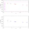 |
Fig. 9 Correlation of the frequency position of the maximum νmax (upper panel) and of the crossover ν0 (lower panel) of the non-thermal SZE from RG lobes as a function of the electron spectrum index α for the seven objects we study here. The lowest frequency Herschel-SPIRE band ( ≈ 447 − 666 GHz, as enclosed by the magenta lines) is shown for comparison. |
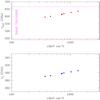 |
Fig. 10 Correlation of the frequency position of the maximum νmax (upper panel) and of the crossover ν0 (lower panel) of the non-thermal SZE from RG lobes as a function of the electron energy density at the center of the radio lobes for the seven objects we study here. The lowest frequency Herschel-SPIRE band ( ≈ 447 − 666 GHz, as enclosed by the magenta lines) is shown for comparison. |
A similar correlation is also found, consistent with the theoretical results described in Sect. 2.1, between ν0 and νmax and the energy density ℰ of the electron population in the radio lobes (see Fig. 10). The analytical formulae with a polynomial of power 2 that fit the frequency locations of νmax and ν0 as a function of ℰ are  (35)and
  (36)where the energy densities are given in keV cm-3 and frequencies in GHz. An analogous correlation with the pressure of the electron population is expected because P = ℰ/3.
The values of ν0 and νmax decrease with increasing values of α and they increase with increasing value of ℰ. This is because the ICS of more energetic electron populations (which have lower values of α, i.e., harder spectra) provide on average a larger frequency increase to the CMB photons (see Colafrancesco et al. 2003; Colafrancesco 2008; Colafrancesco & Marchegiani 2010, for details). The presence and the specific value of a possible high-energy cutoff of the electron spectrum do not change the previous results appreciably for steep electron spectra because they do not affect the value of the total pressure and energy of the electron population.
Table 5 reports, for the same objects we consider in the previous figures, the values of the central synchrotron brightness Ssync at 150 and 500 GHz (evaluated under the assumptions previously described) that we compare with the central SZE brightness change ΔI evaluated at the same frequencies. The values of the brightness are computed using a uniform spatial distribution of the electrons within the assumed ellipsoidal geometry, a uniform magnetic field, and we normalized the electron spectrum with k0 = 2.6 cm-3. We also assume a power-law electron spectrum with a spectral index α indicated in Table 5 and a minimum momentum p1 = 1. These results allow the cases to be identified in which the synchrotron emission either dominates over the SZE signal or provides an appreciable correction to the SZE signal. We find, in agreement with the results of Colafrancesco (2008), that for RG lobes with steep spectra the synchrotron emission provides a negligible contamination of the SZE signal at both 150 and 500 GHz. However, in lobes with flat spectra the synchrotron emission becomes more important. In some cases (e.g., for 3C 292, which is the flattest spectra RG lobes we consider with α = 2.76), it dominates over the SZE signal even at high frequencies. There are also cases (like 3C 274.1 with an intermediate value of α = 2.94) in which the flat spectrum of the electron population provides a substantial contamination to the SZE signal at low frequency (150 GHz), but not at higher frequency (500 GHz).
We stress again that we obtained these results by extrapolating at 150 and 500 GHz the electron spectral index measured at lower radio frequencies (of a few GHz). Therefore, the predicted synchrotron flux in the radio lobes must be considered as an upper limit to the realistic synchrotron signal at high frequencies, which is likely to be steeper due to electron losses and aging (e.g., Longair 1993).
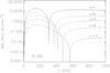 |
Fig. 11 SZE spectrum of 3C 292 for a fixed value of α = 2.76 and for values of p1 = 1 (solid), 2 (dashes), 3 (dot-dashes), 5 (3 dots-dashes) and 10 (long dashes). |
We find that the SZE spectral shape also depends on the minimum momentum p1 (see also Colafrancesco & Marchegiani 2010, 2011, for a discussion of this effect). However, since the value of p1 is unknown, but likely close to its minimum possible value, we assumed in the previous calculations a unique value p1 = 1 for the electron spectrum of all the RG lobes. Because we used an electron population with a power-law spectrum and with a minimum momentum p1 = 1, the electrons that mostly contribute to the SZE signal are those with low momenta, i.e., with p ~ 1. For this reason the crossover frequency of the non-thermal SZE is found at relatively low frequencies, ν0 ~ 300 GHz, for all the objects we consider. Increasing the minimum value of p1 has the effect of moving the values of νmin, ν0 and νmax toward higher frequencies because the electronic population is more populated by higher energy electrons, which thus yield larger frequency up-shifts to the CMB photons. We show this effect for the reference case of the RG 3C 292 in Fig. 11. The fit to the frequency dependence of the main spectral signatures of the SZE (i.e., νmin, ν0, and νmax) for a fixed value of the electron spectral slope α = 2.76 (as for the case of 3C 292) are 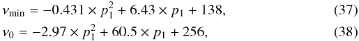 and
and  (39)The frequency values of νmin,ν0, and νmax are given in GHz. The previous fits are valid in the range p1 = 1 ÷ 10, based on the curves reported in Fig. 11. In this case, the minimum of the SZE also increases its location in frequency with increasing values of p1, even if its dependence on p1 is milder than for the other two spectral signatures ν0 and νmax. This effect is due to the fact that the minimum of the SZE is found in the Rayleigh-Jeans parts of the CMB (upscattered and unscattered) spectrum, whose difference is weakly sensitive to the larger distortions of the CMB spectrum produced by the ICCMB process for high-energy electrons. The dependence of νmin from p1 remains unchanged by varying α. The same holds for the dependence of ν0 from p1, but with a shift in the initial value; the dependence of νmax on p1 is instead steeper (flatter) for lower (larger) values of α.
5. The multi-frequency ICS spectrum of RG lobes
In order to establish a more robust normalization of the SZE signals predicted for the RG lobes, we calculate the multi-frequency spectrum of the ICCMB emission in the energy bands where observations are already performed or can be performed, i.e., the soft X-ray band (SXR: 2 − 10 keV), the hard X-ray band (HXR: 20 − 80 keV) and the gamma-ray band (GRB: 0.1 − 100 GeV). Table 6 reports the ICCMB flux produced by the relativistic electrons filling the radio lobes in the SXR, HXR, and GRB energy bands, together with the electron spectral index α for each one of the 21 RG lobes listed in Table 1. These ICS fluxes are calculated with a fixed B-field of 1 μG analogous to the SZE signal calculated in Table 1.
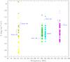 |
Fig. 12 ICS flux predicted for the 21 RG lobes in Table 1 in the SXR, HXR, and gamma-ray bands is compared to the instrumental sensitivity of Swift-XRT, Swift-BAT, and Fermi-LAT. Open dot mark the RG lobes with FICS(1 GeV) larger than the Fermi-LAT sensitivity. The black diamonds mark the seven RGs for which we perform a detailed study. We plot the gamma-ray flux at 1 GeV and the X-ray flux at the centers of the 2−10 keV and 20−80 keV energy bands. The SZE flux is calculated at 150 GHz. |
The predicted ICS flux from about half of the RG lobes in Table 1 overcomes the Fermi-LAT 5yr sensitivity limit at 1 GeV (see Fig. 12). This therefore requires renormalizing the electron spectrum of the RG lobes at the electron energy corresponding to a 1 GeV emitted photon by ICCMB, i.e., at Ee = (1 GeV/8 keV)1/2 ≈ 354 GeV. The electron spectrum normalization for these RG lobes is thus an upper limit on their actual spectrum, given the fact that it is set at the value of the Fermi-LAT sensitivity. The synchrotron frequency corresponding to this energy is ≈1.99 × 10³ GHz, above the frequency range probed by available space experiments.
The electrons in these RG lobes can therefore have either a power-law spectrum extending beyond this energy but renormalized to the Fermi-LAT upper limit or a cutoff at this energy in order to be consistent with the multi-frequency limits. After this renormalization, several RG lobes have SXR and HXR flux still detectable with operative instruments (e.g., Chandra, XMM-Newton, Swift-XRT) and with upcoming HXR instruments (e.g., NuSTAR).
The SZE observations for the RG lobes will thus be relevant in determining their high-energy features.
As previously discussed, the ICCMB spectra of the seven RG lobes reported in Figs. 2–8 for which we perform a detailed analysis are normalized instead to a fixed electron density k0 = 2.6 cm-3. The relative values of the B-field that fit the radio observations are given in Table 3 (we used the previous normalization as a reference value that provides the observed synchrotron flux for Hercules A for a B-field of 1 μG).
For three of the RGs listed in Table 6 there are high-energy observations available that allow the degeneracy between the relativistic electron density and the magnetic field present in synchrotron radio observations to be broken. As a result, the electron spectrum normalization and the RG lobe magnetic field can be determined by combining radio and X-ray observations. Here, we assume that the X-ray flux is due to to ICCMB emission, as in the case of other RGs (see discussion in Sect. 1). Figures 13–15 show the ICS SEDs normalized to the available X-ray data that yield the following electron spectrum normalization: k0 = 4.6 × 10⁻³ cm-3 for 3C 292, k0 = 3.3 cm-3 for 3C 294, and k0 = 2.5 × 10⁻¹ cm-3 for Hercules A. We note (see Erlund et al. 2006, for a detailed analysis) that the X-ray emission associated with 3C 294 is offset in angle compared with the radio emission, so that the normalization k0 for this object should be considered as an upper limit. In addition, the lobes of Hercules A need to have an electron spectrum with a normalization that makes the X-ray and gamma-ray ICCMB emission consistent with the Fermi-LAT limit. Interestingly, the Fermi limit is consistent with a normalization of the ICCMB flux at the lowest observed X-ray flux for Hercules A (see Fig. 15).
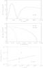 |
Fig. 13 Same as Fig. 2 but for 3C 292 and with normalization to X-ray data. The ICS X-ray emission model is normalized to the X-ray flux from the RG lobe (Croston et al. 2005). |
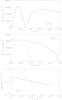 |
Fig. 14 Same as Fig. 2 but for 3C 294 and with normalization to X-ray Chandra data (Gilmour et al. 2009). |
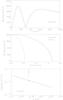 |
Fig. 15 Same as Fig. 2 but for Hercules A and with normalization to the lowest value of the X-ray flux at 2 keV (Feigelson & Berg 1983). |
Given these normalizations for the electron density in these RG lobes, we can estimate the value of the (uniform) B-field in the same lobes by combining the X-ray (ICCMB) flux and the radio synchrotron flux to obtain: B = 2.7 μG for 3C 292, B = 0.41 μG for 3C 294, and B = 3.0 μG for Hercules A (see Table 3). The B-field estimated for 3C 294 is likely larger than B = 0.41 μG because the X-ray flux is an upper limit to the X-ray ICCMB flux from the RG lobe. The B-field estimated for Hercules A is also probably larger than B = 3.0 μG because the X-ray flux used to normalize the ICS emission is likely an upper limit to the X-ray ICS flux from the RG lobe. We emphasize that these estimates of the B-field rely upon the extrapolation of a unique electron spectrum from the energies at which the electrons produce ICS X-ray emission, i.e., Ee ≈ a few tenths of GeV to a GeV, to those at which electrons produce synchrotron emission, i.e., Ee ≈ several to many GeV (see Sect. 1 and the discussion in Colafrancesco & Marchegiani 2011).
The SZE spectra and surface brightness distribution of the three RG lobes calculated using the previous re-normalized values of k0 are shown in Figs. 13–15. In this context, however, observations of the SZE in the lobes of radio galaxies can provide a better and more reliable estimate of the absolute normalization of the electron spectrum and of the RG lobe magnetic field. This is because the SZE is a measure of the integrated electron spectrum and hence less sensitive to the extrapolation of the electron spectrum when comparing the electrons responsible for the synchrotron and X-ray ICCMB emissions.
In the next section, we discuss the optimal observational strategy to determine the full spectrum of the SZE from RG lobes in order to derive the physical parameters of the electron population contained in these systems and to further determine the full physical structure of the RG lobes.
6. Observational strategy
In this section, we discuss a possible observational strategy to study the SZE from the RG lobes. The determination of the full properties of the SZE spectrum from the relativistic electrons populating the RG lobes requires combining observations in the microwave, mm, and sub-mm frequency ranges.
Figure 16 shows the SZE spectra evaluated for the seven RG lobes (under the same assumption used in Figs. 2−8) superposed to the frequency bands in which Planck (yellow), OLIMPO (green), and Herschel-SPIRE (magenta) operate. The optimal frequency channels to study the non-thermal SZE from RG lobes are at ~150 GHz and ≳ 500 GHz, where there is optimal coverage of these instruments.
The Planck-HFI instrument has various frequency bands of interest for studying this SZE signal. These are the bands B2 at 143 ± 30 GHz, B3 at 217 ± 3 GHz, B4 at 353 ± 28 GHz, and B5 at 545 ± 31 GHz. Actually, the Planck-HFI instrument covers the whole frequency range ~100−857 GHz, with NEΔTCMB from ~ to ~
to ~ (see, e.g., The Planck Core Team 2001). However, the highest frequency bands are heavily affected by instrumental and confusion noise.
The SPIRE instrument on board Herschel (see, e.g., Griffin et al. 2010) is a FTS spectrometer with three bands (from 600 to 1200 GHz). It is therefore well suited to observe the SZE from RG lobes, especially the high-ν (positive) region of the SZE, which contains crucial astrophysical information on the electron plasma.
OLIMPO is a balloon-borne experiment carrying a four-band bolometer array that is sensitive to four frequency bands with a band width of ~10%: 150, 220, 340, and 450 GHz (see Masi et al. 2005, 2008; Nati et al. 2007). The OLIMPO instrument is being upgraded, including a differential Fourier-Transform spectrometer similar to the one proposed for the SAGACE space mission project (de Bernardis et al. 2010). The two input ports of a Martin-Puplett interferometer are located in symmetrical positions on the focal plane of the telescope. In this way, the instrument measures the difference of the spectra from couples of pixels (symmetrical with respect to the meridian passing through the center of the focal plane). The resolution of this instrument is 1.8 GHz, and spectra are obtained simultaneously for the four bands of OLIMPO. With such an improvement, the instrument is converted effectively in a 180-band instrument.
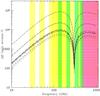 |
Fig. 16 Superposition of the SZE spectrum for the seven objects we consider in our detailed analysis of the non-thermal SZE from RG lobes: 3C 292 (solid), 3C 294 (dots), 3C 274.1 (short dashes), 7C 1602+3739 (long dashes), 87GB 121815+635745 (dot-dashes), B2 1358+30C (dot-long dashes), and Hercules A (short-long dashes). The frequency coverage of Planck (yellow), OLIMPO (green), and Herschel-SPIRE (magenta) are also shown for comparison. |
The combination of these three experiments allows the relevant parts of the RG lobes SZE to be covered, from the frequency region of its minimum (at ν ~ 140 GHz) to the maximum of the SZE (at ν ~ 500−600 GHz). It also probes the tail of the SZE spectrum up to 1200 GHz (see Fig. 16), even though the 857 and 1200 GHz channels are quite susceptible to foreground contamination. This experimental combination allows all the parameters of the non-thermal SZE in RG lobes to be determined: the electron optical depth (mostly from low-frequency data) and the energetics and pressure of the electron population (mostly from high-frequency data). Planck can cover most of the RG lobe SZE spectrum with good sensitivity, especially at ν ≲ 450 GHz, but has a spatial resolution of several arcmin that does not allow a morphological analysis of the SZE from RG lobes. Such a morphological analysis is more suitable with OLIMPO and Herschel-SPIRE. At low and intermediate frequencies, the OLIMPO observations are crucial to determine the minimum of the SZE that provides a measure of the electron optical depth quite independent from the electron energetics (see Fig. 11). At high frequencies, the Herschel-SPIRE observations are crucial to provide information on the energetics and total pressure of the electron population because: i) the SZE spectrum peaks at ~600 GHz (see Figs. 9, 10, 16) and extends in the SPIRE frequency band, so that three high-quality data points can be obtained to describe the smooth shape of the SZE spectrum; ii) the SZE brightness extends for several arcmins and depends only on the spatial distribution of the electrons. The spatial resolution of the Herschel-SPIRE instrument (36.6′′ at 600 GHz, 24.9′′ at 857 GHz, and 18.1′′ at 1200 GHz) can also map the spatial distribution of the SZE and determine the distribution of the electron population and its total energy content, a goal that is not easily feasible with both radio (because of the degeneracy between electrons and B-field) and X-ray or gamma-ray (because only high-E electrons contribute) observations.
Detailed observations of RG lobes in the microwave and mm frequency range have not been obtained so far. Such observations are very relevant to set constraints on the SZE in a frequency region that is marginally affected by synchrotron emission for the steep-spectrum RG lobes, which are the best candidates for a detection of their SZE. We analyze in the following the WMAP 7 yr data to set constraints on the SZE from the seven RG lobes we consider in Table 5 at frequencies of 41, 70, and 94 GHz.
6.1. WMAP constraints
The WMAP 7 yr data in the direction of the RG lobes can set limits on the amplitude of the SZE at μwaves and hence on the value of the minimum momentum p1 (or the momentum break pb for a double power-law spectrum) of the electron spectrum in the RG lobes. In turn, it can set limits on the relevant quantities that depend on it, namely, the electron optical depth, pressure, and energy density. We then use these limits on the electron spectrum to derive more reliable predictions for the shape and amplitude of the SZE spectrum of these RG lobes observable with Planck, OLIMPO, and Herschel-SPIRE.
The WMAP Q, V, and W band maps centered on the seven objects reported in Table 5 are shown in Figs. 17, 18. The total flux of the source is evaluated within a 1 deg2 box centered on the RG lobe center.
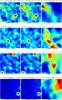 |
Fig. 17 CMB-subtracted WMAP Q (left), V (middle), and W (right) band maps of the seven objects in Table 5. From top to bottom: 3C 274.1, 3C 292, 3C 294, 7C 1602+3739. |
We derive an upper limit on the amplitude of the SZE only in the W band at 90 GHz by subtracting the synchrotron emission (extrapolated from lower-frequency radio observations) to the limit derived from the WMAP 7 yr maps and evaluated within a 1 deg2 box centered on the RG lobe center. We considered the WMAP W channel at 90 GHz because this is the frequency at which the SZE signal is expected to be stronger and the synchrotron signal is expected to be smaller. The SZE flux are calculated using a value of the electron spectrum normalization k0 = 2.6 cm-3 fixed for all the objects that have no information in X-rays, and with the specific value of k0 derived in Sect. 4 for the three objects with X-ray data, i.e., 3C 292, 3C 294, and Hercules A. The SZE fluxes are then set equal to the derived WMAP W-band limit by adjusting the value of p1. This procedure allows the minimum value of p1 (for a single power-law spectrum) for which the total lobe flux does not overcome the WMAP W-band limit to be derived. We also derived, analogously, the minimum value of the break, pb, for a double power-law spectrum with p1 = 1 and α1 = 0 at low electron momenta). The resulting values of p1 and pb are reported in Table 7.
The SZE spectra calculated for a single power-law electron spectrum with the values of p1 obtained from the upper limit of WMAP at 90 GHz in Table 7, are shown in Figs. 19–21. Different values of p1 produce different values of the optical depth, pressure, and energy density of the electron population, which is reflected in different spectral shapes of the SZE in the RG lobes. For objects with increasing values of p1, we find that the SZE spectrum is modified with respect to the one shown in Figs. 2–8, which was obtained with the same electron spectrum energy range, both in amplitude and in spectral shape. In particular, in agreement with the discussion in Sect. 3.2 and Fig. 11, the crossover frequency ν0 is found at frequencies higher than the case when p1 = 1. In the cases in which its value is particularly high (e.g., the cases of 87GB 121815.5+635745, B2 1358+30C), the amplitude of the positive part of the SZE at ν ~ 800−1000 GHz is dramatically reduced compared to the other cases. This effect of p1 on the spectral shape can be verified by measurements of the SZE in the range 400−850 GHz obtainable with Planck, OLIMPO, and Herschel-SPIRE. Therefore, the possible detection (or even additional limits) of the positive part of the SZE in these RG lobes will better constrain the electron spectrum and can fully determine the physical parameters of the electron plasma in the RG lobes (e.g., the value of p1).
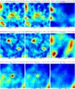 |
Fig. 18 CMB-subtracted WMAP Q (left), V (middle), and W (right) band maps of the seven objects in Table 5. From top to bottom: 87GB 121815.5+635745, B2 1358+30C, Hercules A. |
We also notice that the values of p1 and pb found with the WMAP limits correspond to quite low values of the electron energies: the maximum value of the minimum momentum (pb in this case) for 87GB 121815.5+635745 corresponds to a value of the electron energy of ~50 MeV. For these energies, the electrons in the radio lobes emit synchrotron radiation in the radio frequencies and produce ICCMB emission in the X-ray energies at frequencies (energies) lower than the frequency range at which the lobe emission is actually observed. For the previous case of 50 MeV electrons and for a magnetic field of 0.21 μG (see Table 3), the spectral break at radio frequencies should be found at ~9 kHz, while the ICCMB emission break should be found at ~0.02 keV. For all the other objects we consider here, the spectral breaks should be visible at even lower frequencies (energies) that cannot be observed with radio and X-ray instruments. We can conclude, therefore, that the SZE study of these RG lobes provides the best method to determine the spectral break or the lower cutoff p1 of the electron population for these systems.
Values of p1 and pb derived from the WMAP W-band limits.
6.2. Visibility analysis
We analyze in this section the detectability of the SZE signals expected for the set of RG lobes selected from Tables 5 and 7 with the experimental set-up provided by Planck, OLIMPO, and Herschel. Table 8 shows the SZE signals expected from these RG lobes in the frequency channels from 100 to 857 GHz covered by the combination of Planck-HFI, OLIMPO, and Herschel-SPIRE. For each experiment, we report the signals (in units of mJy/beam) expected from each source in the frequency channels of the various instruments. The values of the signal-to-noise (S/N) ratio for the various instruments is also given in parentheses at each frequency channel. For each frequency channel, we considered the appropriate beam of the instrument; for Planck, we concentrated only on the HFI channels since these have the highest spatial resolution. The expected signals were calculated using the SZE spectra shown in Figs. 19–21, obtained with the complete multi-ν limits at μwaves, X-rays, and gamma-rays.
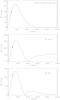 |
Fig. 19 Absolute value of the SZE spectrum integrated over the whole source region for the RGs 87GB 121815.1+635745 (top), 3C 274.1 (mid), and 3C 292 (bottom) calculated for a single power-law spectrum with the values of p1 reported in Table 7. We plot the upper limits derived from the WMAP W-band data. |
The flux error calculated for a 1-hour integration with OLIMPO is 1.61, 1.79, 0.54, and 0.29 mJy/beam at ν = 143,217,353, and 450 GHz, respectively, and the confusion noise (assumed to be dust dominated) is 0.2, 0.76, 3.32, and 7.19 mJy/beam at the same frequency channels. For the Planck-HFI instrument, we calculate a flux error for a 14-month integration time of 3.97, 2.81, 3.88, 7.34, 14.29, and 16.67 mJy/beam at ν = 100,143,217,353,545, and 857 GHz, respectively. The confusion noise (assumed to be dust dominated) at the same Planck-HFI frequency channels is 0.09, 0.26, 0.95, 6.68, 37.94, and 231.99 mJy/beam. For the Herschel-SPIRE instrument, the detector noise is negligible with respect to the confusion noise levels of 6.80, 6.30, and 5.80 mJy/beam at ν = 600,857,1200 GHz. The S/N ratio for each instrument channel is reported in parentheses after the value of the expected SZE flux.
SZE signals for the restricted set of RG lobes expected in the Planck, OLIMPO, and Herschel-SPIRE instruments.
We find that most of the RG lobes have an SZE well detectable up to 353 GHz with both OLIMPO and Planck, while the S/N ratio decreases to values of ≲ a few or even below 1 at higher frequencies, where both the intrinsic noise of the instruments and the confusion noise largely increase. The Herschel-SPIRE instrument is therefore crucial to detect the SZE signals from RG lobes at higher frequencies >600 GHz. For this instrument, the expected S/N ratios are significantly larger than 1, except in the case of RG 87GB 121815.5+635745. This RG lobe has a very steep electron spectrum with a power-law index α = 3.9, the largest among the selected RG lobes, which given the WMAP W band limit requires a rather large value of p1. This value depresses the SZE signal in the high-frequency region. As verification of this trend we notice that the RG with the smaller electron spectrum cutoff (i.e., 3C 294 with p1 = 1.4) shows the largest expected SZE signal in all the frequency channels of the Herschel-SPIRE instrument.
6.3. Confusion and biases
Possible sources of confusion of the SZE signal on the spatial scales of the RG lobes we consider here include the synchrotron emission from the same RG lobes, CMB fluctuations, point-like sources and the diffuse Galaxy emission. The synchrotron emission from the RG lobes does not contribute substantially to the level of confusion of the SZE signals at 150 GHz, and even less at higher frequency ≳500 GHz (see Tables 2 and 4). The CMB fluctuations on the angular scales (~1 to 15 arcmin) of RG lobes do not provide a sensitive level of confusion. In addition they have a flat spectrum that can be efficiently separated from the RG lobe SZE signal.
The Galaxy emission is the major source of contamination. However, since most of the RG lobes are selected to be at high galactic latitudes, we can reasonably think that this source of confusion could be also separated from the SZE signals by knowing its spectral behavior.
The level of unresolved point source contamination is more difficult to establish and depends also on the model assumed for the sub-mm and mm source evolution with redshift. However, the recent HERSCHEL-SPIRE results provide an estimate of the confusion at the levels of 5.8, 6.3, and 6.8 mJy/beam at 250, 350, and 500 μm, respectively. The beams of the instrument are 18.1, 24.9, and 36.6 arcsec (FWHM) at 250, 350, and 500 μm (N’guyen et al. 2010).
In the estimate of the SZE signals expected for the seven RG lobes with Planck, OLIMPO, and Herschel-SPIRE (see Table 8), we considered the confusion caused by unresolved dusty galaxies; this confusion is more relevant for OLIMPO and Planck than for Herschel-SPIRE.
We conclude that the level of confusion of the RG lobe SZE signal is marginal at low frequencies (150 GHz), relevant at the level of intermediate frequencies (~300−400 GHz where the crossover is found), and dominant at high frequencies (≳500 GHz). At these high frequencies, most of the astrophysical information on the RG lobes can be extracted by studying the relative SZE spectral shape. We find that the RG lobes whose ICS spectra require low values of the minimum momentum cutoff p1, which are consistent with observations and upper limits at multi-frequency, are the objects more easily detectable in all the frequency channels of the three experiments we considered here. Therefore, they offer the best targets to recover their overall SZE spectrum from microwaves to sub-mm ranges.
7. Discussion and conclusions
We have presented in this paper the first extensive study of the relativistic SZE in RG lobes that makes use of the available observational constraints over a wide frequency range, from radio and microwave to X-ray and gamma-ray frequency bands. The constraints on the electron spectral slope and on the intensity at microwaves (i.e., at 90 GHz from the WMAP W-band), X-ray, and gamma-ray (i.e., Fermi-LAT) allow limits to be derived for the value of the electron spectrum normalization and the minimum electron momentum p1, and in turn for the amplitude and spectral shape of the SZE in RG lobes. The inclusion of X-ray observations from some of the RG lobes in our sample (assuming that the X-ray flux data are produced by ICCMB) further allow realistic estimates on the overall value of the magnetic field in the RG lobes to be established. They also enable accurate determination of the spectrum of the relativistic electrons over a wide range of energies that fit the radio synchrotron emission, the ICCMB X-ray, and the gamma-ray emission limits from RG lobes. With these constraints, we determined the realistic spectrum and amplitude of the non-thermal SZE in the RG lobes considered in our analysis.
A detailed visibility analysis of the SZE for the selected RG lobes showed that balloon-borne and space-borne experiments like Planck-HFI, OLIMPO, and Herschel-SPIRE will be able to determine accurately the SZE spectral characteristics in many RG lobes and open the way to the vast astrophysical and cosmological use of this specific SZE signal.
The largest expected SZE signals from RG lobes occur at microwaves (in the region of its minimum at ~ 150 − 170 GHz) and in the sub-mm range (in the region of the quite flat maximum at ν ≳ 600 GHz, which also could be extended at higher frequencies depending on the electron spectral cutoff p1). The combination of Planck, Herschel-SPIRE, and OLIMPO provides an excellent framework to study the SZE from giant RG lobes and demonstrates the importance of future experiments in the mm and sub-mm range with spatially resolved spectroscopic capabilities.
Future SZE observations of RG lobes will be crucial for the determination of the energetics, pressure, and spatial distribution of relativistic electrons in the RG lobes, and hence for the description of the very high-E phenomena associated with these systems. Knowing the SZE spectra will allow the total energy and spectrum of the relativistic electrons in RG lobes to be measured, because the SZE depends on the total pressure/energy density of the electronic population along the los through the lobe. SZE measurements provide much more accurate estimates of the electron pressure/energy density than techniques like ICCMB X-ray emission or synchrotron radio emission, since the former can only provide an estimate of the electron energetics in the high-energy part of the electron spectrum, and the latter is sensitive to the degenerate combination of the electron spectrum and of the magnetic field in the radio lobes (see Colafrancesco & Marchegiani 2011).
We have shown that the combination of the SZE and radio observations of RG lobes also allow the magnetic field structure in RG lobes to be determined more reliably than the combination of ICCMB X-ray (or gamma-ray) and radio emission. This is because the SZE is a measure of the total energy density, i.e., an integral over the whole electron spectrum. X-ray observations in a fixed energy band, however, can provide an estimate of the electron spectrum in a slice of the electron spectrum that does not fit with the electron energy range probed by radio synchrotron observations  (Bμ is the magnetic field expressed in μG) unless very high B-fields are present in the radio lobes (see Colafrancesco & Marchegiani 2011). Specifically, an electron of energy Ee can produce both ICS and synchrotron emission for a value of the magnetic field
  (40)which requires magnetic field values of order of ~255 to 2550 μG to perform observations at an X-ray energy of EX = 0.2 keV and for radio observations in the range 0.1 − 1 GHz. The assumption of a constant slope of the electron spectrum from the energies probed by radio observations (i.e., ~ several to many GeV) down to the energies probed by ICS X-ray observations (i.e., ~ tenths to a GeV) is required to use the relation FICS/Fsynch = ℰCMB/ℰB, which provides the estimate for the magnetic field energy density ℰB, given the known value of the CMB radiation energy density ℰCMB. For three of the seven RGs that we consider in detail, this technique allows the value of the (uniform) B-field to be derived at the level of ≈ 2.7 (for 3C 292), ≳ 3.0 (for Hercules A), and ≳ 0.41 (for 3C 294) μG.
The spatially resolved study of the SZE and the synchrotron emission in the lobes of RGs can provide indications on the radial behavior of both the leptonic pressure and the magnetic field from the inner parts to the boundaries of the lobes. The study of the pressure evolution in radio lobes can give crucial information on the transition from radio-lobe environments to the atmospheres of giant cavities observed in galaxy cluster atmospheres (see, e.g., McNamara & Nulsen 2007, for a review), which seem naturally related to the penetration of RG jets/lobes into the intra-cluster medium.
The detection of the SZE from RG lobes also has a relevant cosmological implication since it can be used, in combination with ICS X-ray emission measurements, to measure the evolution of the CMB temperature at each RG redshift (as proposed by Colafrancesco 2008). The possibility to detect RG lobes at high redshifts then allows the evolution of TCMB(z) to be probed in the early ages of the cosmic history. This possibility, coupled to the study of TCMB(z) at low and moderate redshifts by using galaxy clusters (see, e.g., Battistelli et al. 2003) allows a reconstruction of a large part of the cosmic evolution of the CMB radiation field and of the possible energy injections at early and late epochs.
Preliminary studies of the SZE in RG lobes are limited so far to a few cases at radio frequency (see, e.g., Yamada et al. 2010). The low frequency of these observation do not permit non-thermal SZE to be detected because of the low expected brightness of these signals in this part of the e.m. spectrum. However, the next generation radio telescopes like SKA with sensitivity ≲ μJy and wide spectral coverage, ~0.5−45 GHz, will be able to provide crucial information on the low-ν part of the SZE spectrum and its polarization level (Colafrancesco et al., in prep.). The SZE from RG lobes could be also observed with mm arrays like ALMA, especially in small-size lobes with dimensions matching the ALMA field of view. Even though the specific sources we selected in this paper are located in the northern hemisphere and thus not visible by SKA and/or ALMA, it will be relevant for the detailed study of the RG lobes to have a simultaneous observation of RG lobes from ~0.4 GHz to ~40 GHz, as well as in the ALMA 1 − 3 bands, with arcsec spatial resolution in order to disentangle the diffuse synchrotron emission from the relative ICS emission. This strategy will allow the spatial and energy distribution of the relativistic electron population to be separated from that of the magnetic field in RG lobes. We will address this issue in more detail for SKA and ALMA in a forthcoming paper (Colafrancesco et al., in prep.).
We finally stress the strong complementarity between SZE observations and high-E observations of the ICCMB emission in RG lobes, which are possible mainly in the X-rays (Chandra), hard X-rays (NuSTAR, Astro-H) and in the gamma-rays (Fermi, HESS, CTA). The preliminary studies of the μwave–mm and X-ray – gamma-ray emission from RG lobes will allow to
determine the full energy spectrum of the electronic population in RG lobes and their interaction properties with external radiation and magnetic fields. We will address this important issue in a future study.
The case of 3C 294 should be considered with caution because the X-ray emission associated with this RG is not co-spatial with the radio lobes (see Erlund et al. 2006). However, this X-ray emission is likely a mixture of extended (i.e., associated with the lobes) and compact (i.e., associated with the core) emission.
Acknowledgments
We thank an anonymous referee for several useful comments and suggestions that allowed us to improve the discussion and the presentation of our results. S.C. acknowledges support by the South African Research Chairs Initiative of the Department of Science and Technology and National Research Foundation and by the Square Kilometre Array. Our research was also supported by contracts OLIMPO I/004/07/1 and Planck-HFI I/030/10/0 of the Italian Space Agency.
References
- Abdo, A. A., Ackermann, M., Ajello, M., et al. 2010, Science, 328, 725 [NASA ADS] [CrossRef] [PubMed] [Google Scholar]
- Abramowitz, M., & Stegun, I. A. 1965, Handbook of Mathematical Functions with Formulas, Graphs and Mathematical Tables (New York: Dover Book) [Google Scholar]
- Battistelli, E. S., De Petris, M., Lamagna, L., et al. 2002, ApJ, 580, L101 [NASA ADS] [CrossRef] [Google Scholar]
- Birkinshaw, M. 1999, Phys. Rep., 310, 97 [NASA ADS] [CrossRef] [Google Scholar]
- Blundell, K. M., & Fabian, A. C. 2011, MNRAS, 412, 705 [NASA ADS] [Google Scholar]
- Blundell, K. M., Fabian, A. C., Crawford, C. S., et al. 2006, ApJ, 644, L13 [NASA ADS] [CrossRef] [Google Scholar]
- Colafrancesco, S. 2008, MNRAS, 385, 2041 [NASA ADS] [CrossRef] [Google Scholar]
- Colafrancesco, S., & Marchegiani, P. 2010, A&A, 520, 31 [Google Scholar]
- Colafrancesco, S., & Marchegiani, P. 2011, A&A, 535, 108 [NASA ADS] [CrossRef] [EDP Sciences] [Google Scholar]
- Colafrancesco, S., Marchegiani, P., & Palladino, E. 2003, A&A, 397, 27 [NASA ADS] [CrossRef] [EDP Sciences] [Google Scholar]
- Comastri, A., Brunetti, G., Dallacasa, D., et al. 2003, MNRAS, 340, L52 [NASA ADS] [CrossRef] [Google Scholar]
- Croston, J. H., Birkinshaw, M., Hardcastle, M. J., & Worrall, D. M. 2004, MNRAS, 353, 879 [NASA ADS] [CrossRef] [Google Scholar]
- Croston, J. H., Hardcastle, M. J., Harris, D. E., et al. 2005, ApJ, 626, 733 [NASA ADS] [CrossRef] [Google Scholar]
- De Bernardis, P., et al. 2010 [arXive:1002.0867] [Google Scholar]
- Ensslin, T., & Kaiser, C. 2000, A&A, 360, 417 [NASA ADS] [Google Scholar]
- Erlund, M. C., Fabian, A. C., et al. 2006, MNRAS, 371, 29 [NASA ADS] [CrossRef] [Google Scholar]
- Feigelson, E. D., & Berg, C. J. 1983, ApJ, 269, 400 [NASA ADS] [CrossRef] [Google Scholar]
- Gilmour, R., Best, P., & Almaini, O. 2009, MNRAS, 392, 1509 [NASA ADS] [CrossRef] [Google Scholar]
- Govoni, F., & Feretti, L. 2004, IJMPD, 13, 1549 [NASA ADS] [CrossRef] [Google Scholar]
- Guidetti, D., et al. 2011, MNRAS, 413, 2525 [NASA ADS] [CrossRef] [Google Scholar]
- Griffin, M. J., Abergel, A., Abreu, A., et al. 2010, A&A, 518, L3 [Google Scholar]
- Hardcastle, M. J., & Croston, J. H. 2005, MNRAS, 363, 649 [NASA ADS] [Google Scholar]
- Harris, D. E., & Grindlay, J. E. 1979, MNRAS, 188, 25 [NASA ADS] [Google Scholar]
- Harris, D. E., & Krawczynski, H. 2002, ApJ, 565, 244 [NASA ADS] [CrossRef] [Google Scholar]
- Ishiwara-Chandra, C. H., & Saikia, D. J. 1999, MNRAS, 309, 100 [NASA ADS] [CrossRef] [Google Scholar]
- Kardashev, N. S. 1962, SvA, 6, 317 [Google Scholar]
- Kataoka, J., & Stawarz, L. 2005, ApJ, 622, 797 [NASA ADS] [CrossRef] [Google Scholar]
- Kataoka, J., Leahy, J. P., Edwards, P. G., et al. 2003, A&A, 410, 833 [NASA ADS] [CrossRef] [EDP Sciences] [Google Scholar]
- Kronberg, P. P., Colgate, S. A., Li, H., Dufton, Q. W., et al. 2004, ApJ, 604, L77 [NASA ADS] [CrossRef] [Google Scholar]
- Laing, R., & Peacock, J. A. 1980, MNRAS, 190, 903 [NASA ADS] [CrossRef] [Google Scholar]
- Longair, M. 1993, High Energy Astrophysics (Cambridge: Cambridge University Press) [Google Scholar]
- Masi, S., Calvo, M., Conversi, L., et al. 2005, in 17th ESA Symposium on European Rocket and Balloon Programmes and Related Research, ed. B. Warmbein (Noordwijk: ESA Pub. Division), ESA SP-590, 581 [Google Scholar]
- Masi, S., Battistelli, E., Brienza, D., et al. 2008, MemSAIt, 79, 887 [NASA ADS] [Google Scholar]
- McKinnon, M. M., Owen, F. N., & Eilek, J. A. 1991, AJ, 101, 2026 [NASA ADS] [CrossRef] [Google Scholar]
- McNamara, B. R., & Nulsen, P. E. J. 2007, ARA&A, 45, 117 [NASA ADS] [CrossRef] [MathSciNet] [Google Scholar]
- Miley, G. 1980, ARA&A, 18, 165 [Google Scholar]
- Nati, F., Ade, P., Boscaleri, A., et al. 2007, NewAR, 51, 385 [NASA ADS] [CrossRef] [Google Scholar]
- N’guyen, H. T., Schulz, B., Levenson, L., et al. 2010, A&A, 518, L5 [NASA ADS] [CrossRef] [EDP Sciences] [Google Scholar]
- Planck HFI Core team 2011, A&A, 536, A4 [NASA ADS] [CrossRef] [EDP Sciences] [Google Scholar]
- Schoenmakers, et al. 2000, A&AS, 146 [Google Scholar]
- Schlickeiser, R. 2002, Cosmic ray astrophysics (Berlin: Springer) [Google Scholar]
- Yamada, M., Fujita, Y., Matsuo, H., & Sugiyama, N. 2010, AJ, 139, 2494 [NASA ADS] [CrossRef] [Google Scholar]
All Tables
SZE signals for the restricted set of RG lobes expected in the Planck, OLIMPO, and Herschel-SPIRE instruments.
All Figures
|
Fig. 1 SZE brightness change ΔI/I is shown as a function of the observed radio spectral index αr for the RG lobes in Table 1. The various panels refer to the cases p = 1,10,100,1000 from top down. Black triangles refer to SZE decrement at 150 GHz (in modulus) while the blue asterisks refer to the SZE increment at 500 GHz for p1 = 1 and to the SZE decrement at 500 GHz (in modulus) for p1 = 10, 100, and 1000. The SZE signals in Table 1 are all evaluated for a fixed value of the RG lobe magnetic field (B = 1 μG uniform in the emission region for all the objects considered). |
| In the text | |
|
Fig. 2 Upper panel: SZE spectrum at the center of the radio galaxy lobe 87GB 121815.5+635745. Mid panel: SZE signal profile at 150 GHz calculated along the major axis (solid line) and along the minor XIS (dashed line). Lower panel: the ICS-on-CMB flux produced by the relativistic electron population in the radio lobes of this object. |
| In the text | |
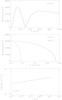 |
Fig. 3 Same as Fig. 2 but for 3C 274.1. |
| In the text | |
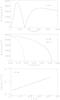 |
Fig. 4 Same as Fig. 2 but for 3C 292. |
| In the text | |
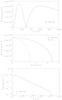 |
Fig. 5 Same as Fig. 2 but for B2 1358+30C. |
| In the text | |
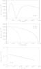 |
Fig. 6 Same as Fig. 2 but for 3C 294. |
| In the text | |
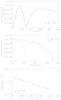 |
Fig. 7 Same as Fig. 2 but for 7C 1602+3739. |
| In the text | |
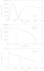 |
Fig. 8 Same as Fig. 2 but for Hercules A. |
| In the text | |
|
Fig. 9 Correlation of the frequency position of the maximum νmax (upper panel) and of the crossover ν0 (lower panel) of the non-thermal SZE from RG lobes as a function of the electron spectrum index α for the seven objects we study here. The lowest frequency Herschel-SPIRE band ( ≈ 447 − 666 GHz, as enclosed by the magenta lines) is shown for comparison. |
| In the text | |
|
Fig. 10 Correlation of the frequency position of the maximum νmax (upper panel) and of the crossover ν0 (lower panel) of the non-thermal SZE from RG lobes as a function of the electron energy density at the center of the radio lobes for the seven objects we study here. The lowest frequency Herschel-SPIRE band ( ≈ 447 − 666 GHz, as enclosed by the magenta lines) is shown for comparison. |
| In the text | |
|
Fig. 11 SZE spectrum of 3C 292 for a fixed value of α = 2.76 and for values of p1 = 1 (solid), 2 (dashes), 3 (dot-dashes), 5 (3 dots-dashes) and 10 (long dashes). |
| In the text | |
|
Fig. 12 ICS flux predicted for the 21 RG lobes in Table 1 in the SXR, HXR, and gamma-ray bands is compared to the instrumental sensitivity of Swift-XRT, Swift-BAT, and Fermi-LAT. Open dot mark the RG lobes with FICS(1 GeV) larger than the Fermi-LAT sensitivity. The black diamonds mark the seven RGs for which we perform a detailed study. We plot the gamma-ray flux at 1 GeV and the X-ray flux at the centers of the 2−10 keV and 20−80 keV energy bands. The SZE flux is calculated at 150 GHz. |
| In the text | |
|
Fig. 13 Same as Fig. 2 but for 3C 292 and with normalization to X-ray data. The ICS X-ray emission model is normalized to the X-ray flux from the RG lobe (Croston et al. 2005). |
| In the text | |
|
Fig. 14 Same as Fig. 2 but for 3C 294 and with normalization to X-ray Chandra data (Gilmour et al. 2009). |
| In the text | |
|
Fig. 15 Same as Fig. 2 but for Hercules A and with normalization to the lowest value of the X-ray flux at 2 keV (Feigelson & Berg 1983). |
| In the text | |
|
Fig. 16 Superposition of the SZE spectrum for the seven objects we consider in our detailed analysis of the non-thermal SZE from RG lobes: 3C 292 (solid), 3C 294 (dots), 3C 274.1 (short dashes), 7C 1602+3739 (long dashes), 87GB 121815+635745 (dot-dashes), B2 1358+30C (dot-long dashes), and Hercules A (short-long dashes). The frequency coverage of Planck (yellow), OLIMPO (green), and Herschel-SPIRE (magenta) are also shown for comparison. |
| In the text | |
|
Fig. 17 CMB-subtracted WMAP Q (left), V (middle), and W (right) band maps of the seven objects in Table 5. From top to bottom: 3C 274.1, 3C 292, 3C 294, 7C 1602+3739. |
| In the text | |
|
Fig. 18 CMB-subtracted WMAP Q (left), V (middle), and W (right) band maps of the seven objects in Table 5. From top to bottom: 87GB 121815.5+635745, B2 1358+30C, Hercules A. |
| In the text | |
|
Fig. 19 Absolute value of the SZE spectrum integrated over the whole source region for the RGs 87GB 121815.1+635745 (top), 3C 274.1 (mid), and 3C 292 (bottom) calculated for a single power-law spectrum with the values of p1 reported in Table 7. We plot the upper limits derived from the WMAP W-band data. |
| In the text | |
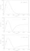 |
Fig. 20 Same as Fig. 19, but for the RGs B2 1358+300 (top), 3C 294 (mid), and 7C 1602+3739 (bottom). |
| In the text | |
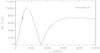 |
Fig. 21 Same as Fig.19, but for the RG Hercules A. |
| In the text | |
Current usage metrics show cumulative count of Article Views (full-text article views including HTML views, PDF and ePub downloads, according to the available data) and Abstracts Views on Vision4Press platform.
Data correspond to usage on the plateform after 2015. The current usage metrics is available 48-96 hours after online publication and is updated daily on week days.
Initial download of the metrics may take a while.