| Issue |
A&A
Volume 549, January 2013
|
|
|---|---|---|
| Article Number | A10 | |
| Number of page(s) | 10 | |
| Section | Planets and planetary systems | |
| DOI | https://doi.org/10.1051/0004-6361/201219996 | |
| Published online | 06 December 2012 | |
The transiting system GJ1214: high-precision defocused transit observations⋆, and a search for evidence of transit timing variation⋆⋆
1
Niels Bohr Institute, University of Copenhagen,
Juliane Maries vej 30,
2100
Copenhagen Ø,
Denmark
e-mail: This email address is being protected from spambots. You need JavaScript enabled to view it.
2
Centre for Star and Planet Formation, Natural History Museum of
Denmark, Øster Voldgade
5, 1350
Copenhagen,
Denmark
3
Korea Astronomy and Space Science Institute,
776 Daedeokdae-ro, Yuseong-gu,
305-348
Daejeon, Republic of
Korea
4
Astrophysics Group, Keele University, Staffordshire, ST5 5BG, UK
5
SUPA, University of St Andrews, School of Physics &
Astronomy, North
Haugh, St Andrews,
KY16
9SS UK
6
Department of Physics, Sharif University of
Technology, PO Box
11155-9161, Tehran,
Iran
7
Max-Planck-Institute for Solar System Research,
Max-Planck Str. 2, 37191
Katlenburg-Lindau,
Germany
8
Qatar Foundation, Doha,
Qatar
9
Dipartimento di Fisica “E. R. Caianiello”, Università di
Salerno, via Ponte Don
Melillo, 84084
Fisciano (SA),
Italy
10
HE Space Operations GmbH, Flughafenallee 24, 28199
Bremen,
Germany
11
Istituto Nazionale di Fisica Nucleare, Sezione di
Napoli, Napoli,
Italy
12
Istituto Internazionale per gli Alti Studi Scientifici
(IIASS), 84019
Vietri Sul Mare (SA),
Italy
13
Institut für Astrophysik, Georg-August-Universität
Göttingen, Friedrich-Hund-Platz
1, 37077
Göttingen,
Germany
14
European Southern Observatory, Karl-Schwarzschild-Straße 2, 85748
Garching bei München,
Germany
15
Institut d’Astrophysique et de Géophysique, Université de
Liège, 4000
Liège,
Belgium
16
Astronomisches Rechen-Institut, Zentrum für Astronomie,
Universität Heidelberg, Mönchhofstraße 12-14, 69120
Heidelberg,
Germany
17
Max Planck Institute for Astronomy, Königstuhl 17, 69117
Heidelberg,
Germany
18
Jodrell Bank Centre for Astrophysics, University of
Manchester, Oxford
Road, Manchester,
M13 9PL,
UK
19
Space Telescope Science Institute, 3700 San Martin Drive, Baltimore, MD
21218,
USA
20
Stellar Astrophysics Centre (SAC), Department of Physics and
Astronomy, Aarhus University, Ny
Munkegade 120, 8000
Aarhus C,
Denmark
21
National Astronomical Observatories/Yunnan Observatory, Chinese
Academy of Sciences, 650011
Kunming, PR
China
22
Perimeter Institute for Theoretical Physics,
31 Caroline St. N.,
Waterloo ON, N2L 2Y5, Canada
23
Southwest Research Institute, Department of Space
Studies, 1050 Walnut St., Suite
400, Boulder,
CO
80302,
USA
Received:
12
July
2012
Accepted:
5
October
2012
Abstract
Aims. We present 11 high-precision photometric transitobservations of the transiting super-Earth planet GJ 1214 b. Combining these data with observations from other authors, we investigate the ephemeris for possible signs of transit timing variations (TTVs) using a Bayesian approach.
Methods. The observations were obtained using telescope-defocusing techniques, and achieve a high precision with random errors in the photometry as low as 1 mmag per point. To investigate the possibility of TTVs in the light curve, we calculate the overall probability of a TTV signal using Bayesian methods.
Results. The observations are used to determine the photometric parameters and the physical properties of the GJ 1214 system. Our results are in good agreement with published values. Individual times of mid-transit are measured with uncertainties as low as 10 s, allowing us to reduce the uncertainty in the orbital period by a factor of two.
Conclusions. A Bayesian analysis reveals that it is highly improbable that the observed transit times is explained by TTV caused by a planet in the nominal habitable zone, when compared with the simpler alternative of a linear ephemeris.
Key words: planetary systems / stars: individual: GJ1214 / methods: statistical / methods: observational / techniques: photometric
By the MiNDSTEp collaboration from the Danish 1.54 m telescope at the ESO La Silla Observatory.
Photometric data used in the light curves are only available at the CDS via anonymous ftp to cdsarc.u-strasbg.fr (130.79.128.5) or via http://cdsarc.u-strasbg.fr/viz-bin/qcat?J/A+A/549/A10
Royal Society University Research Fellow.
© ESO, 2012
1. Introduction
The transiting exoplanet GJ 1214 b was discovered in 2009 by the MEarth project1 (Charbonneau et al. 2008). This planet transits a nearby M dwarf (Charbonneau et al. 2009), with a mass 0.15 M⊙ and the planet is generally classified as a super-Earth with a mass and radius (Mp = 6.37 M⊕ and Rp = 2.74 R⊕ according to Kundurthy et al. (2011), in this study we find Mp = 6.26 M⊕ and Rp = 2.85 R⊕) between that of Earth and Neptune, a type of planet that has no solar system analogue. GJ 1214 b is one of the lowest temperature transiting exoplanets known and, as it is also detectable with radial velocity (RV) methods – a very interesting target for detailed study.
Due to the relatively low mean density of GJ 1214 b, ρp = 1.49 ± 0.33 g cm-3 in this study, it has been suggested to hold some extended atmosphere or gaseous envelope. But the planet composition in this mass and radius range is degenerate (Adams et al. 2008), warranting further studies in order to determine its composition. Defining what the atmosphere consists of can help determine the planet composition. Rogers & Seager (2010) describes three possibilities for the interior and atmospheric composition of GJ 1214 b. It could be (1) a mini-Neptune with a H/He gas envelope; (2) a “water world” with a water-rich and ice-dominated interior and a water-vapour-dominated envelope; or (3) a rocky planet with an atmosphere mainly consisting of H2.
Log of the transit observations of GJ 1214 for this work.
Recent results from among others the Kepler mission (Latham et al. 2011) and gravitational microlensing (Gould et al. 2010) gives reason to believe that multiple systems are common. It is therefore inherently interesting to look for traces of transit timing variations in any transiting system and especially so in GJ 1214, as the planet seems to be at the inner edge of the habitable zone, with an equilibrium temperature of in the region of 393 to 555 K (Charbonneau et al. 2009), i.e. finding a planet in a slightly larger orbit would be very interesting.
Additional planets can be revealed via their gravitational effects on the transiting planet. This would result in telltale systematic deviations in the mid-transit times from a linear ephemeris, a phenomenon known as transit timing variation (TTV) (Agol et al. 2005; Holman & Murray 2005). GJ 1214 b is well-suited to such an analysis due to its short transits, allowing precise measurements of mid-transit times, and its short period, which means many transits are observable. One disadvantage is
its relative faintness, which could cause a loss of precision in the measured transit times.
We have gathered photometric observations of 11 transits in the GJ 1214 system, and modelled them to estimate the transit times. Inclusion of results from the literature leads to a total time interval of 833 days over which TTVs can be investigated. In the following work we cast the problem of detecting a TTV signal as a model selection problem and via Bayesian methods calculate the probability that the data, as a whole, actually contain a TTV signal.
In Sect. 2 we present the new data and their reduction, which in Sect. 3 are analysed in order to obtain new transit times and physical properties. Section 4 contains a description of the Bayesian model selection process.
2. Observations and data reduction
We observed five transits of GJ 1214 b in the period of 2010 July 6th to 2011 June 3rd, using the Danish 1.54 m telescope at ESO La Silla and the focal-reducing camera DFOSC. The plate scale of DFOSC is 0.39″ per pixel. The full field of view is 13.7′ × 13.7′, but for each transit observation the CCD was windowed down to reduce the readout time from around 90 s to approximately 30 s. The four transits in 2010 were observed through a Cousins I filter, while the 2011 transit was observed in Johnson R. An observing log is given in Table 1.
The transits were observed with the telescope defocused, in order to use longer exposure times whilst avoiding CCD saturation. This approach allowed us to decrease the Poisson and scintillation noise by exposing for a larger fraction of the time during transit (see Southworth et al. 2009). The impact of flat-fielding errors was minimised by the use of defocusing and by autoguiding the telescope throughout the observations. The diameters of the defocused point spread functions (PSFs) ranged from 31 to 42 pixels.
We also observed one transit of GJ 1214 b using the 1.52 m Cassini Telescope at the Loiano Observatory, Italy. The BFOSC CCD imager was used, and was defocused with the same approach as taken for the Danish telescope observations (see Southworth et al. 2010).
One transit was observed simultaneously in the g, r and z filters using the Calar Alto 2.2 m telescope and the BUSCA four-beam CCD imager. A fourth dataset was obtained in the u-band but, as expected, yielded a light curve which was too noisy to be useful. For further discussion on the observing strategy we used for BUSCA please see Southworth et al. (2012).
Finally, one transit was observed in 2010 using the GROND seven-beam imager on the 2.2 m MPI telescope at ESO La Silla. The observations were performed without telescope defocusing. Useful results could be obtained for only the r and i filters, with the star proving too faint in the g, z and JHK channels.
The data were reduced using the pipeline described in Southworth et al. (2009), which performs standard aperture photometry with the astrolib/aper2idl routine. A range of aperture sizes were tried, and the ones which gave the least noisy light curves were adopted (Table 1). The form of the transit is insensitive to the choice of aperture sizes, and to the presence of two faint stars within the sky annulus.
Comparison stars to be used for relative photometry were chosen within the field, and the astrolib/aper routine determined relative magnitudes for these and GJ 1214, from the given coordinates and aperture radius. Potential comparison stars that proved to be variable or too faint were discarded. Relative photometry of GJ 1214 was obtained against an optimally weighted ensemble of comparison stars.
The resulting GJ 1214 light curve does not have a constant magnitude out of transit, primarily due to changes in airmass and intrinsic stellar variability. To correct any systematic trends, the out-of-transit data points were fitted with a straight line. Simultaneous optimisation of the comparison star weights and the out-of-transit polynomial was used to obtain the final light curves, which are shown in Fig. 1.
Three additional light curve were obtained from the Exoplanet Transit Database3 (Poddaný et al. 2010). These were contributed by Johannes Ohlert (2010/07/18) and Thomas Sauer (2010/06/29 and 2010/07/07).
3. Light curve analysis
3.1. Analysis with JKTEBOP
The light curves were analysed with the jktebop4 code (Southworth et al. 2004a,b), originally developed as ebop (Etzel 1981; Popper & Etzel 1981) for modelling light curves of detached eclipsing binaries. The use of the code for exoplanet transit light curves is discussed in detail in Southworth (2008).
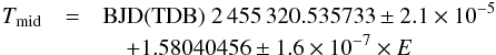
The size of the planet relative to the size of the star is directly related to the transit depth. jktebop models the sky projections of the two objects as biaxial spheroids, dividing them into concentric circles and assigning a limb darkening to each of the rings before estimating the flux. With optical observations of a planetary system, it is safe to assume that the secondary object, the exoplanet, is dark, so the surface brightness ratio can thus be set to zero. Using jktebop we fitted for the inclination i of the orbit, the sum and ratio of the fractional radii k = rp + r ⋆ and rp/r ⋆ . The fractional radii are rp = Rp/a and r ⋆ = R ⋆ /a, where Rp and R ⋆ are the absolute planetary and stellar radii, respectively, and a is the semi-major axis of the orbit. We also fitted for the time of minimum of each light curve, Tmid, using a fixed orbital period of P = 1.58040490 days (Berta et al. 2011). The mass ratio, which only affects the shape of the ellipsoids describing the components, was fixed at q = 0.0002, which is sufficiently close to the value 0.00013 found in this paper. We found that changes, less than one order of magnitude, in this value have a negligible effect on the results.
Limb darkening (LD) affects the shape of a transit light curve. LD will cause the bottom of the transit to have a curved shape. We tried fitting four different LD laws: linear, square-root, logarithmic and quadratic. LD coefficients can be found from stellar atmosphere models given the effective temperature and surface gravity. Only Claret (2000, 2004) provides LDCs for stars as cool as GJ 1214 A. We used values for a star of Teff = 3000 K and log g = 5.00 (cgs units).
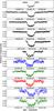 |
Fig. 1 The 11 observed transit light curves of GJ 1214 b, plotted in the same order as listed in the observing log in Table 1. For the observations taken in multiple filters simultaneously the datapoints are coloured in spectral order, i.e. blue for bluest etc. |
Photometric parameters of GJ 1214 from the best-fitting light curves to the 2010-season data from the Danish telescope.
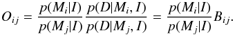
We analysed the combined 2010 Danish telescope data, finding that one LD coefficient could be included as a fitted parameter. We therefore fitted for the linear coefficient whilst holding the nonlinear coefficient fixed at the theoretical value. For the other datasets we had to fix both coefficients in order to avoid unphysical results. The best fits to the Danish telescope data are plotted in Fig. 2.
In order to obtain uncertainties in the fitted parameters we first rescaled the error bars of the datapoints to give a reduced χ2 of unity for each transit light curve. This step is necessary because the data errors returned by the aper algorithm are normally too small. We then performed 1000 Monte Carlo simulations (see Southworth et al. 2004b) on each light curve to derive the errorbars in the fitted parameters quoted in Table 2.
The light curve from 2010/07/06 was unintentionally obtained using an exposure time of 150 s, which is significant compared to the duration of the ingress and egress. When fitting these data we used the possibility within jktebop to numerically integrate the light curve model in order to obtain an unbiased fit (Southworth 2011).
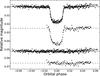 |
Fig. 2 Combined Danish telescope light curve of the 2010 data (top) and the 2011 light curve (bottom), versus the best jktebop fit (solid lines 2010, dashed 2011) with the logarithmic LD law. The residuals to the fits are plotted below, where the lines mark zero residual. |
3.2. Physical properties of the system
It is possible to calculate the physical properties of the GJ 1214 system from our
measured photometric parameters and from published values of the stellar effective
temperature, metal abundance and orbital velocity amplitude. We obtained final values for
r ⋆ , rp and
i from our results for the 2010 Danish Telescope data. Each was
calculated as the mean of the values from the solutions using the four LD laws, with the
uncertainty being the quadrature sum of the largest individual uncertainty plus the
standard deviation of the four individual parameter values. For the star we adopted the
temperature Teff = 3026 ± 150 K and orbital velocity amplitude
K ⋆ = 12.2 ± 1.6 m s-1 from
Charbonneau et al. (2009), and the metal abundance
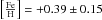 from Rojas-Ayala et al. (2010).
The physical properties were then calculated by requiring the properties of the star to match the tabulated predictions of the DSEP stellar evolutionary models (Dotter et al. 2008). This step was performed using the procedure outlined by Southworth (2009). The DSEP model set was chosen because it is the only one of the five sets used by Southworth (2010) which reaches to sufficiently low stellar masses.
The input and output parameters for this analysis are given in Table 3 and show a reasonable agreement with literature values. The mass, radius and surface gravity of the star are given by M ⋆ , R ⋆ and log g ⋆ , respectively. The mass, radius, surface gravity and mean density of the planet are denoted by Mp, Rp, gp and ρp, respectively.
The measured physical properties will be subject to systematic errors as theoretical evolutionary models are not perfect representations of reality. Southworth (2009) found that this systematic error was generally 1% or less for the masses and radii of transiting planets and their host stars. In the case of GJ 1214 this systematic error could be significantly larger, due to the relatively poorer theoretical understanding of 0.2 M⊙ stars, but will still be significantly smaller than the statistical uncertainties quoted in Table 3.
3.3. Orbital period determination
The times are given in barycentric Julian days (BJD), and have been calculated from UTC
with codes provided by Eastman et al. (2010). By
augmenting our measured Tmid values with ones from the
literature (Table 4), we are able to refine the
orbital ephemeris for GJ 1214, refitting for P and
T0 the zero epoch:
 (1)where
E is the orbit count with respect to the reference epoch. The reduced
χ2 for this fit is 1.24. The estimated period is identical
to the previous estimates, but the uncertainty on the period P has been
reduced by approximately a factor of two (Berta et al.
2011; Carter et al. 2011; Kundurthy et al. 2011). The fit and the residuals are
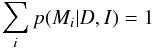
plotted in Fig. 3. Given the rather large spread in
data points compared with the period, one would not expect this estimate of the period to
be afflicted by significant systematic error. On the other hand the
T0 could have systematic error, which is handled in the
later Bayesian analysis by marginalising out this parameter.
(1)where
E is the orbit count with respect to the reference epoch. The reduced
χ2 for this fit is 1.24. The estimated period is identical
to the previous estimates, but the uncertainty on the period P has been
reduced by approximately a factor of two (Berta et al.
2011; Carter et al. 2011; Kundurthy et al. 2011). The fit and the residuals are
plotted in Fig. 3. Given the rather large spread in
data points compared with the period, one would not expect this estimate of the period to
be afflicted by significant systematic error. On the other hand the
T0 could have systematic error, which is handled in the
later Bayesian analysis by marginalising out this parameter.
4. Transit timing variation as Bayesian model selection
A system with a transiting planet enables the possibility of detecting additional unseen planets in the timing data by TTVs, that is, look for systematic trends in the residuals of Fig. 3. We will in the following outline a method for quantitatively assessing the probability of whether such a signal exists in the timing dataset or not.
One could simply fit an appropriate function describing mutual gravitational perturbations, and evaluate a measure like the classical squared sum of residuals. But it is, in general, true that a model with more free parameters will be able to fit noise better, i.e. produce a lower squared sum of residuals by fitting nonphysical features. The problem is especially prominent when the sought effect is on the same order as the uncertainty in the data, in which case it is not easy to determine how much of an improvement in the squared sum of residuals one should demand for a more complex model to be plausible.
Derived physical properties of the GJ 1214 system.
Mid-transit times from the literature and the present work.
One is forced to penalise models for having too many parameters. Thus the problem is no longer a problem of parameter estimation, but a problem of model selection. One needs to apply Occam’s razor. One formal way of doing so is via Bayesian model selection, which is completely analogous to, but distinct from, Bayesian parameter estimation. Whilst it might not be possible to estimate the parameters of a model with any certainty, a wide range of plausible parameters which do improve the squared residuals by some amount would lend credibility to the notion that the model in question is true. How true can be expressed as a probability.
The search for a TTV signal can conveniently be cast as a model selection problem. If there is a TTV signal there has to be some kind of pattern in the residuals listed in Table 4. The expected signal from perturbation from another body can be calculated with an N-body orbital mechanics code.
4.1. Bayesian estimation
4.1.1. Parameter estimation
Following the development in (Chap. 3 Gregory 2005), Bayesian parameter estimation can conceptually be thought of as testing a range of mutually excluding hypotheses Hi, i.e. one assumes a parametrised model M. This model can be thought of as a logical disjunction (“or”) M = H1 + H2 + ... where the hypothesis Hi implies that a given parameter θ has the particular value θi.
For mutually exclusive probabilities the sum rule applies. Assuming that the parameter
θ does indeed take a value, one can write
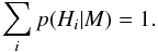 (2)From Bayes’
theorem one learns that
(2)From Bayes’
theorem one learns that 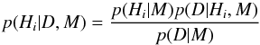 (3)where
the left hand side
p(Hi | D,M)
is the posterior probability of Hi, i.e.
the probability of the hypothesis Hi in the
light of the data D. The term
p(D | Hi,M)
is the probability of the data D if
Hi true. This quantity is known as the
likelihood of Hi. The term
p(Hi | M)
is known as the prior and represents the probability one assigns to
Hi in the light of one’s model before
any data becomes available. Finally the term in the denominator
p(D | M) is known as the global
likelihood or the evidence.
(3)where
the left hand side
p(Hi | D,M)
is the posterior probability of Hi, i.e.
the probability of the hypothesis Hi in the
light of the data D. The term
p(D | Hi,M)
is the probability of the data D if
Hi true. This quantity is known as the
likelihood of Hi. The term
p(Hi | M)
is known as the prior and represents the probability one assigns to
Hi in the light of one’s model before
any data becomes available. Finally the term in the denominator
p(D | M) is known as the global
likelihood or the evidence.
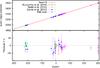 |
Fig. 3 Times of mid-transit from the literature and this work. In the upper plot the errorbars are smaller than the point marker and are thus not shown. The lower plot shows the residuals on a different scale. Some of the observations are taken with instruments that simultaneously observe in several filters so some of the data points coincide in time. |
Based on assumptions one can deduce the value of
p(D | M)
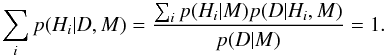 (4)Thus
 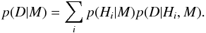 (5)That is, the
denominator, which does not depend on the individual hypotheses
Hi, is the sum of the numerator over
Hi. The process of summing over all the
hypothesis is known as marginalisation. It is clear that the evidence serves as a
normalisation constant. For parameter estimation this normalisation is unimportant, as
in most cases one simply seeks the maximum posterior value without regard to
normalisation. But for model selection this evidence term is important.
(5)That is, the
denominator, which does not depend on the individual hypotheses
Hi, is the sum of the numerator over
Hi. The process of summing over all the
hypothesis is known as marginalisation. It is clear that the evidence serves as a
normalisation constant. For parameter estimation this normalisation is unimportant, as
in most cases one simply seeks the maximum posterior value without regard to
normalisation. But for model selection this evidence term is important.
4.1.2. Model selection
Model selection is carried out following the exact same procedure as above, only assuming a disjunction of models I = M1 + M2 + ... + MN, instead of a disjunction of hypotheses.
Bayes’ theorem now reads 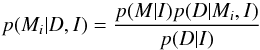 (6)one
immediately recognises the second term in the numerator as the evidence term from Eq.
(5). Just as the probability of a
parameter is proportional to the likelihood times the prior, the probability of a model
is proportional to the evidence times the prior. The denominator in Eq. (6) can be calculated like the evidence in Eq.
(5), assuming that one of the
Mi is the true model. In other words the
probability of a model is given by marginalising over all the parameters in the model.
(6)one
immediately recognises the second term in the numerator as the evidence term from Eq.
(5). Just as the probability of a
parameter is proportional to the likelihood times the prior, the probability of a model
is proportional to the evidence times the prior. The denominator in Eq. (6) can be calculated like the evidence in Eq.
(5), assuming that one of the
Mi is the true model. In other words the
probability of a model is given by marginalising over all the parameters in the model.
Often it is more convenient to work with odds ratios O and Bayes
factors B defined as
 (7)Assuming that
 (8)one can write
the probabilities of the individual models as
(8)one can write
the probabilities of the individual models as 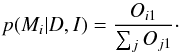 (9)It is crucial to notice
that these odds ratios implicitly result in an Occam’s razor. One may notice that the
evidence term in Eq. (5) takes the form
of an average of the likelihood over the prior. Hence penalising complicated models by
their unused prior space, e.g. large swathes of prior space with negligible likelihood,
will pull down the average of the likelihood over the prior. In other words, the more
plausible model is the one that makes more sharp predictions with fewer adjustable
parameters. Note that the form of the priors and the prior ranges are as much part of
the model specification as the functional form of the likelihood function, which is no
surprise given that probabilities are purely a function of one’s state of knowledge.
There is nothing inherent in nature about probabilities. Also note that assigning
probabilities according to Eq. (9), i.e.
normalising to a total sum of one, implicitly assumes that one of the models is true.
(9)It is crucial to notice
that these odds ratios implicitly result in an Occam’s razor. One may notice that the
evidence term in Eq. (5) takes the form
of an average of the likelihood over the prior. Hence penalising complicated models by
their unused prior space, e.g. large swathes of prior space with negligible likelihood,
will pull down the average of the likelihood over the prior. In other words, the more
plausible model is the one that makes more sharp predictions with fewer adjustable
parameters. Note that the form of the priors and the prior ranges are as much part of
the model specification as the functional form of the likelihood function, which is no
surprise given that probabilities are purely a function of one’s state of knowledge.
There is nothing inherent in nature about probabilities. Also note that assigning
probabilities according to Eq. (9), i.e.
normalising to a total sum of one, implicitly assumes that one of the models is true.
4.1.3. MultiNest
The mainstay of Bayesian posterior distribution evaluation has for many years been Monte Carlo methods, in particular Monte Carlo Markov chain (MCMC) algorithms. Unfortunately it turns out that most MCMC incarnations generally have trouble accurately estimating the evidence term, in particular when the posterior has multiple modes. Indeed many of the various MCMC packages available do not directly calculate the evidence term.
As noted before, the estimation of parameters does not require one to calculate the evidence term, but model selection does. A recent innovation in Monte Carlo methods is the MultiNest algorithm, which is specifically designed to accurately evaluate evidences (Feroz & Hobson 2008; Feroz et al. 2009).
4.2. Application of Bayesian model selection to TTV search
TTVs arise from the dynamics of a planetary system if there is more than one planet in the system. But as it is commonly known, the three body problem and higher is chaotic over long time scales. Such a signal could show up as a change in apparent orbital period, or the phase of the orbit.
Given these ambiguities we have then chosen to frame the search for a TTV signal as a Bayesian model selection problem. To every transit we observe we can unambiguously assign an epoch, given prior information on the orbital period, which in the case of GJ 1214 b is approximately 1.5804 days. We have calculated the probability of the linear no-TTV model versus models with TTV simulated with an N-body code.
4.2.1. Non-TTV model
Assuming no transit timing variation, we would expect that the relation between the time of mid-transit and the epoch is perfectly linear. In the Bayesian framework presented above, given the distribution of errors and the prior ranges, we can calculate the probability of this particular model itself and compare it directly to the probability of the model with a TTV signal.
As the prior ranges are included in the overall posterior probabilities of the models it is necessary to assign ranges to these priors, i.e. the posterior probability takes the form of an average of the likelihood over the prior; see Eq. (5).
The parameter T0 in both the models is related to the definition of the epoch. It is simply the Julian date of the mid-transit of epoch 0. When the epoch is defined, this quantity is in principle known, but we cannot determine it exactly; hence, we introduce a systematic error. In a Bayesian framework we can take this into account by marginalising out T0. The prior range of T0 has been chosen to correspond to the largest error in the two measurements that pertain to epoch 0 in Table 4.
4.2.2. TTV models
Unfortunately there is no known analytic solution to the general three body problem. Hence, to calculate the TTV arising to a third perturbing body in the system one has to rely on numerical orbital integration codes. One such code is Swift (Levison & Duncan 1994), which has been employed here. For our purposes we have adapted the FORTRAN code used in Nesvorný & Morbidelli (2008), with this adapted code we where able to satisfactorily reproduce results in that article.
For the purpose of this investigation it was assumed that GJ 1214 b is in a circular orbit, which is likely given the results in Charbonneau et al. (2009) where the eccentricity is estimated to be less than 0.27. Further we assume that GJ 1214 b is perturbed by an planet in a coplanar circular orbit.
Given a trial mass m, period P and mean longitude λ of the hypothetical perturbing planet, and assuming the time of first transit to be t = 0, the provided code calculates the time of all future transits taking into account the gravitational interaction between the planets. In the simple case of two coplanar circular orbits the argument of periapsis simply determines the angular separation of the two planets at the start of the integration. The standard deviation of the TTV signal as a function of these parameters can be calculated numerically as done in Fig. 4.
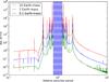 |
Fig. 4 Standard deviation,in units of seconds, of the TTV signal of GJ 1214 b calculated for different masses of the perturber. The various mean motion resonances are clearly visible. The blue shaded area marks perturber orbits that would make the orbit of GJ 1214 b unstable. |
Table of parameters for the non-TTV and two TTV models that have been analysed.
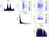 |
Fig. 5 Marginal probability and conditional probabilities for the TTV model assuming an exterior perturber from MultiNest. The parameter T0 is a nuisance parameter, which is integrated out, hence the marginal and conditional probabilities have not been plotted. |
 |
Fig. 6 Marginal probability and conditional probabilities for the TTV model assuming an interior perturber from MultiNest. The parameter T0 is a nuisance parameter, which is integrated out, hence the marginal and conditional probabilities have not been plotted. |
The majority of perturber parameter space will give rise to negligible TTV, but from Fig. 4 two regions of perturber parameter space which can give rise to significant TTV, comparable to the uncertainty of our data, can be identified. One region consists of periods in the range from the 2:1 resonance, at a relative period of 0.5, to the inner edge of the instability strip. The other region is from the outer edge of the instability strip to the 2:1 resonance, at a relative period of 2. In both of these regions, perturbers down to a mass of about 0.1 Earth mass will give rise to TTV of a second or more. Hence we will use these ranges as prior ranges in the model selection. The two regions will be treated as two different models to be tested against each other. The upper mass range for these two models will be set by the accuracy of radial velocity data from Charbonneau et al. (2009), where radial velocity data with a accuracy of about 10 m/s were presented. We estimate that in the outer model, perturbers heavier than 6 Earth masses are excluded and for the inner model, perturbers heavier than 5 Earth masses are excluded by RV data. The two TTV models are presented in Table 5 together with the non-TTV (i.e. linear) model, and their priors.
4.3. Discussion
The final results of these three models have been summarised in Table 5, along with the prior ranges of the parameters. We conclude that there is a very strong preference for the no-TTV model, given the calculated overall probabilities of the three models, because the relatively low quality, in the form of large uncertainties, of the available data does not allow us to reach complicated conclusions.
It should be noted that posterior probability of the model includes these prior ranges, hence the probability of the model can be thought of as the probability that a planet in this part of parameter space explains the transit times of GJ 1214 b. But note that the probability of a model is normalised by the prior volume, so a model with larger prior ranges or more parameters will be less probable, unless heavily supported by data. Large prior ranges are equivalent to lack of prior knowledge, hence one needs strong evidence to accept a complicated model in absence of prior knowledge.
MultiNest is in essence a Monte Carlo code and it does produce posterior samples, which can be analysed similarly to the samples produced by conventional Monte Carlo codes to produce estimates of the posterior probability of the parameters and their correlations. This has been done in Figs. 5 and 6 for the two TTV cases, respectively.
The posterior estimate of the period P in the no-TTV shows good agreement with the estimate produced in Sect. 3.3. To evaluate the evidence term we have marginalised over a range of offsets to take account for the uncertainly in the timing of the zero epoch.
The plot of the posterior probabilities in Figs. 5 and 6 shows the marginal probabilities of the parameters of a perturbing planet, assuming that the data is explained by a perturbing planet within the prior ranges. These marginal probabilities show preference for a light planet (small m). The gaps in the marginal posterior of the period P occurs at strong resonances that would give rise to TTV much larger than what is observed.
5. Conclusions
In this paper we have presented and analysed 11 new transit light curves of the exoplanet GJ 1214 b. In addition new analyses of three previously published transits are presented. With these new data it has been possible to improve the previously estimated ephemeris and physical properties of GJ 1214 and GJ 1214 b. The calculated physical properties are consistent with previously published values and the uncertainty in the orbital period has been reduced by a factor of approximately two – P = 1.58040456 ± 1.6 × 10⁻⁷.
Furthermore a stringent analysis, incorporating available prior knowledge in the form of orbital mechanics and previous RV investigations, of whether transit timing variation can explain the data has been undertaken via Bayesian methods. Specifically we have calculated the probability of three models for explaining the data, two with a TTV and one without, assuming a priori that one of the models is true. This analysis has revealed that the models with TTVs are highly improbable compared to the simple model assuming no TTV. That is, the given data does not allow us to conclude that there is a planet in the mass range 0.1–5 Earth-masses and the period range 0.76–1.23 or 1.91–3.18 days. To be able to reach such conclusions we would need many more consistent data points and/or higher accuracy.
A planet with a greenhouse warming and albedo similar to Earth at a period of approximately 4.5 days in the GJ 1214 system, corresponding to a period relative to GJ 1214 b of 3, would have a surface temperature of about 80 °C. Conversely a planet in this orbit with an albedo similar to Venus and a greenhouse warming of 0 would have a surface temperature of about 0 °C. Hence such a planet could be at the inner or outer edge of the habitable zone of GJ 1214 b depending on the parameters – for high albedo and/or low greenhouse warming the habitable zone overlaps with the region of parameter space that can reasonably be investigated with a transit timing accuracy on the order on 10 s; see Fig. 4. Because of the orbital resonance, habitable planets down to Mars-mass could potentially be revealed in the GJ 1214 b system with the already achieved timing accuracy. To investigate the habitable zone for planets more similar to Earth, a much higher accuracy on the order of 0.01 s is called for.
Distributed within the idl Astronomy User’s Library at http://idlastro.gsfc.nasa.gov/
jktebop is written in fortran77 and the source code is available at http://www.astro.keele.ac.uk/~jkt/
Acknowledgments
In addition to data from the Danish 1.54 m telescope at ESO La Silla Observatory, this article is based on (1) observations collected at the MPG/ESO 2.2 m Telescope located at ESO La Silla, Chile. Operations of this telescope are jointly performed by the Max Planck Gesellschaft and the European Southern Observatory. GROND has been built by the high-energy group of MPE in collaboration with the LSW Tautenburg and ESO, and is operating as a PI-instrument at the MPG/ESO 2.2 m telescope; (2) data collected at the Centro Astronómico Hispano Alemán (CAHA) at Calar Alto, Spain, operated jointly by the Max-Planck Institut für Astronomie and the Instituto de Astrofísica de Andalucía (CSIC); (3) observations obtained with the 1.52 m Cassini telescope at the Astronomical Observatory of Bologna in Loiano, Italy. The authors would like to acknowledge Johannes Ohlert from the Astronomie Stiftung Trebur, Germany and Thomas Sauer from Internationale Amateursternwarte E. V., for graciously contributing datasets from the Michael Adrian Observatory and Observaorium Hakos, respectively, via the Exoplanet Transit Database (Poddaný et al. 2010). J. Southworth acknowledges support from STFC in the form of an Advanced Fellowship. J. Surdej, F. Finet, D. Ricci and O. Wertz acknowledge support from the Communauté française de Belgique – Actions de recherche concertées – Académie universitaire Wallonie-Europe. Research by T. C. Hinse is carried out at the Korea Astronomy and Space Science Institute (KASI) under the KRCF (Korea Research Council of Fundamental Science and Technology) Young Scientist Research Fellowship Program. T. C. Hinse acknowledges support from KASI registered under grant number 2012-1-410-02. The contributions from K. A. Alsubai, M. Dominik, M. Hundertmark and C. Liebig were made possible by NPRP grant NPRP-09-476-1-78 from the Qatar National Research Fund (a member of Qatar Foundation). The statements made herein are solely the responsibility of the authors.
References
- Adams, E. R., Seager, S., & Elkins-Tanton, L. 2008, ApJ, 673, 1160 [NASA ADS] [CrossRef] [Google Scholar]
- Agol, E., Steffen, J., Sari, R., & Clarkson, W. 2005, MNRAS, 359, 567 [NASA ADS] [CrossRef] [Google Scholar]
- Berta, Z. K., Charbonneau, D., Bean, J., et al. 2011, ApJ, 736, 12 [NASA ADS] [CrossRef] [Google Scholar]
- Carter, J. A., Winn, J. N., Holman, M. J., et al. 2011, ApJ, 730, 82 [NASA ADS] [CrossRef] [Google Scholar]
- Charbonneau, D., Irwin, J., Nutzman, P., & Falco, E. E. 2008, in BAAS, 40, AAS Meeting Abstracts, #212, 242 [Google Scholar]
- Charbonneau, D., Berta, Z. K., Irwin, J., et al. 2009, Nature, 462, 891 [NASA ADS] [CrossRef] [PubMed] [Google Scholar]
- Claret, A. 2000, VizieR Online Data Catalog, J/A+A/363/1081 [Google Scholar]
- Claret, A. 2004, A&A, 428, 1001 [NASA ADS] [CrossRef] [EDP Sciences] [Google Scholar]
- Dotter, A., Chaboyer, B., Jevremović, D., et al. 2008, ApJS, 178, 89 [NASA ADS] [CrossRef] [Google Scholar]
- Eastman, J., Siverd, R., & Gaudi, B. S. 2010, PASP, 122, 935 [NASA ADS] [CrossRef] [Google Scholar]
- Etzel, P. B. 1981, in Photometric and Spectroscopic Binary Systems, eds. E. B. Carling, & Z. Kopal, 111 [Google Scholar]
- Feroz, F., & Hobson, M. P. 2008, MNRAS, 384, 449 [NASA ADS] [CrossRef] [Google Scholar]
- Feroz, F., Hobson, M. P., & Bridges, M. 2009, MNRAS, 398, 1601 [NASA ADS] [CrossRef] [Google Scholar]
- Gould, A., Dong, S., Gaudi, B. S., et al. 2010, ApJ, 720, 1073 [NASA ADS] [CrossRef] [Google Scholar]
- Gregory, P. 2005, Bayesian logical data analysis for the physical sciences: a comparative approach with Mathematica support (Cambridge University Press) [Google Scholar]
- Holman, M. J., & Murray, N. W. 2005, Science, 307, 1288 [NASA ADS] [CrossRef] [PubMed] [Google Scholar]
- Kundurthy, P., Agol, E., Becker, A. C., et al. 2011, ApJ, 731, 123 [NASA ADS] [CrossRef] [Google Scholar]
- Latham, D. W., Rowe, J. F., Quinn, S. N., et al. 2011, ApJ, 732, L24 [NASA ADS] [CrossRef] [Google Scholar]
- Levison, H. F., & Duncan, M. J. 1994, Icarus, 108, 18 [NASA ADS] [CrossRef] [Google Scholar]
- Nesvorný, D., & Morbidelli, A. 2008, ApJ, 688, 636 [NASA ADS] [CrossRef] [Google Scholar]
- Poddaný, S., Brát, L., & Pejcha, O. 2010, New A, 15, 297 [Google Scholar]
- Popper, D. M., & Etzel, P. B. 1981, AJ, 86, 102 [NASA ADS] [CrossRef] [Google Scholar]
- Rogers, L. A., & Seager, S. 2010, ApJ, 716, 1208 [NASA ADS] [CrossRef] [Google Scholar]
- Rojas-Ayala, B., Covey, K. R., Muirhead, P. S., & Lloyd, J. P. 2010, ApJ, 720, L113 [NASA ADS] [CrossRef] [Google Scholar]
- Southworth, J. 2008, MNRAS, 386, 1644 [NASA ADS] [CrossRef] [Google Scholar]
- Southworth, J. 2009, MNRAS, 394, 272 [NASA ADS] [CrossRef] [Google Scholar]
- Southworth, J. 2010, MNRAS, 408, 1689 [NASA ADS] [CrossRef] [Google Scholar]
- Southworth, J. 2011, MNRAS, 417, 2166 [NASA ADS] [CrossRef] [Google Scholar]
- Southworth, J., Maxted, P. F. L., & Smalley, B. 2004a, MNRAS, 349, 547 [NASA ADS] [CrossRef] [Google Scholar]
- Southworth, J., Maxted, P. F. L., & Smalley, B. 2004b, MNRAS, 351, 1277 [NASA ADS] [CrossRef] [Google Scholar]
- Southworth, J., Hinse, T. C., Jørgensen, U. G., et al. 2009, MNRAS, 396, 1023 [NASA ADS] [CrossRef] [Google Scholar]
- Southworth, J., Mancini, L., Novati, S. C., et al. 2010, MNRAS, 408, 1680 [NASA ADS] [CrossRef] [Google Scholar]
- Southworth, J., Mancini, L., Maxted, P. F. L., et al. 2012, MNRAS, 422, 3099 [NASA ADS] [CrossRef] [Google Scholar]
All Tables
Photometric parameters of GJ 1214 from the best-fitting light curves to the 2010-season data from the Danish telescope.
All Figures
|
Fig. 1 The 11 observed transit light curves of GJ 1214 b, plotted in the same order as listed in the observing log in Table 1. For the observations taken in multiple filters simultaneously the datapoints are coloured in spectral order, i.e. blue for bluest etc. |
| In the text | |
|
Fig. 2 Combined Danish telescope light curve of the 2010 data (top) and the 2011 light curve (bottom), versus the best jktebop fit (solid lines 2010, dashed 2011) with the logarithmic LD law. The residuals to the fits are plotted below, where the lines mark zero residual. |
| In the text | |
|
Fig. 3 Times of mid-transit from the literature and this work. In the upper plot the errorbars are smaller than the point marker and are thus not shown. The lower plot shows the residuals on a different scale. Some of the observations are taken with instruments that simultaneously observe in several filters so some of the data points coincide in time. |
| In the text | |
|
Fig. 4 Standard deviation,in units of seconds, of the TTV signal of GJ 1214 b calculated for different masses of the perturber. The various mean motion resonances are clearly visible. The blue shaded area marks perturber orbits that would make the orbit of GJ 1214 b unstable. |
| In the text | |
|
Fig. 5 Marginal probability and conditional probabilities for the TTV model assuming an exterior perturber from MultiNest. The parameter T0 is a nuisance parameter, which is integrated out, hence the marginal and conditional probabilities have not been plotted. |
| In the text | |
|
Fig. 6 Marginal probability and conditional probabilities for the TTV model assuming an interior perturber from MultiNest. The parameter T0 is a nuisance parameter, which is integrated out, hence the marginal and conditional probabilities have not been plotted. |
| In the text | |
Current usage metrics show cumulative count of Article Views (full-text article views including HTML views, PDF and ePub downloads, according to the available data) and Abstracts Views on Vision4Press platform.
Data correspond to usage on the plateform after 2015. The current usage metrics is available 48-96 hours after online publication and is updated daily on week days.
Initial download of the metrics may take a while.