| Issue |
A&A
Volume 549, January 2013
|
|
|---|---|---|
| Article Number | A54 | |
| Number of page(s) | 13 | |
| Section | The Sun | |
| DOI | https://doi.org/10.1051/0004-6361/201219307 | |
| Published online | 18 December 2012 | |
Alfvén waves in coronal holes: formation of discontinuities in inhomogeneous magnetic fields
Dipartimento di Fisica, Università della Calabria,
via P. Bucci, 87036
Rende (CS), Italy
e-mail: This email address is being protected from spambots. You need JavaScript enabled to view it.
Received:
29
March
2012
Accepted:
24
October
2012
Abstract
Context. Solar wind fluctuations are characterized by discontinuities. The nature and properties of these structures have been largely studied in the literature, and different mechanisms have been proposed to explain their formation.
Aims. We investigate the evolution of Alfvénic perturbations propagating in the inhomogeneous magnetic field of a coronal open-field region, in order to study both the way that small-scale structures are generated and the possible formation of discontinuities.
Methods. We constructed a model for the equilibrium magnetic field in a coronal hole. The model represents a potential field with a complex structure: regions of opposite polarity or of only the dominant polarity are present at low or high altitudes, respectively. The evolution of small-amplitude Alfvén waves in the inhomogeneous structure is studied by employing a WKB approach that describes how the perturbation wavevector and the wave phase vary along magnetic lines.
Results. We find that small-scale structures form in the perturbation at relatively low altitudes (~3 × 10⁴ km) above the coronal base. An initially monochromatic perturbation develops a steep power-law spectrum with slope α ≃ 2.3, which is strongly anisotropic with a predominance of quasi-perpendicular wavevectors. Small-scale structures are localized around separatrices of the magnetic structures. In many cases they contain quasi-perpendicular rotational discontinuities that can propagate to the upper corona, eventually reaching the solar wind.
Conclusions. The considered mechanism could be responsible for forming a fraction of the population of discontinuities detected in the solar wind.
Key words: magnetohydrodynamics (MHD) / waves / Sun: corona / solar wind
© ESO, 2012
1. Introduction
Alfvénic fluctuations represent the main component of low-frequency perturbations in the solar wind. They are characterized by a strong correlation between velocity and magnetic field fluctuations, as well as a low level (compared with the background values) of density and magnetic-field intensity fluctuations. Alfvénic perturbations in the solar wind have been revealed by in-situ observations for several decades (Belcher & Davis 1971): they dominate low-frequency perturbations both in high-speed streams at lower heliospheric latitudes and in the high-latitude wind. More recently, evidence of Alfvénic fluctuations in the solar corona has been found by Tomczyk & McIntosh (2009). These authors find velocity fluctuations that propagate by following magnetic field lines at a well-defined propagation speed that is consistent with estimations of the Alfvén velocity. Indirect evidence of Alfvén waves in coronal holes has also been reported (see Banerjee et al. 2011, for a review). These observations support the idea that Alfvénic fluctuations observed in the high-speed solar wind that emanates from the open-field corona mostly have a solar origin and are ultimately due to photospheric motions localized underneath the base of the corona. Such fluctuations can be modified when crossing the corona and/or within the solar wind by other phenomena, such as nonlinear effects or interactions with background inhomogenities.
Discontinuities, i.e., abrupt localized changes in physical parameters (e.g., direction and intensity of magnetic field and velocity, density, temperature and plasma composition) are commonly detected in the solar wind. In directional discontinuities (DD), the magnetic field change direction, intensity, or both at once. Within the framework of magnetohydrodynamics (MHD), DDs can be considered to be either rotational (RD) or tangential (TD) discontinuities. The RDs have a finite component of magnetic field Bn in the normal direction and propagate at the Alfvén speed along the mean magnetic field. The velocity and magnetic field variations in RDs are correlated as in Alfvén waves, while pressure and magnetic field intensity are continuous across the discontinuity. The RDs could be considered as Alfvén waves in which the wave phase presents an abrupt variation. The TDs have vanishing normal magnetic field component Bn, and they can have arbitrary jumps in plasma and magnetic pressure, though the sum of these pressures must remain constant across the discontinuity. The TDs do not propagate in the plasma reference frame and can be interpreted as the boundary between two adiacent magnetic flux tubes.
A classification for the observed DDs has been first proposed by Smith (1973) with subsequent modifications, based on the value of the angle θBn (the larger angle between the upstream or downstream magnetic field and the normal direction) and on the relative jump ΔB/B of magnetic field intensity. The DD is a TD for high values of both θBn and ΔB/B (cosθBn < 0.4, ΔB/B > 0.2), while, in the opposite case (cosθBn > 0.4, ΔB/B < 0.2), the DD is an RD. However, for large θBn and small ΔB/B, the DD could be either a TD with a small jump in magnetic field intensity, or it could be a RD propagating at a large angle with respect to the ambient magnetic field. Because of this ambiguity, in this case the DD is classified as an “either discontinuity” (ED).
In single-spacecraft measurements, the minimum variance analysis has been commonly employed to determine the normal direction n, which is chosen as the direction of the eigenvector for the magnetic field variance matrix ⟨ ΔBiΔBj ⟩ corresponding to the lower eigenvalue. Many single-spacecraft studies of DDs in the solar wind have been published (e.g., Burlaga 1969; Smith 1973; Martin et al. 1978; Tsurutani & Smith 1979; Mariani et al. 1983; Neugebauer 1989; Soding et al. 2001): in most cases RDs or TDs have been found to be prevalent in fast-speed or in slow-speed streams, respectively. Using multiple (three or more) spacecraft data allows for determining the normal direction by considering the times of crossing the DD for each spacecraft (Burlaga & Ness 1969; Horbury et al. 2001; Knetter et al. 2003; 2004). Unlike what is found by minimum variance analisys, the multiple-spacecraft technique indicates a prevalence of EDs in the population of DDs with respect to the other kinds of discontinuities (Knetter et al. 2003; 2004). It has been suggested that this discrepancy is due to the inability of the minimum variance methods to find the correct normal orientation when waves are superposed on the discontinuity (e.g., Horbury et al. 2001; Vasquez 2005). In any case, more reliable 3D information on the orientation of the discontinuity is expected to be found using multiple spacecrafts.
Other important aspects of DDs are (e.g., Neugebauer 2006): (i) small relative variations in proton density are associated with small-amplitude discontinuities, which indicates that such discontinuities are essentially noncompressive; (ii) velocity and magnetic field changes across discontinuities are correlated in a similar manner as in Alfvénic fluctuations at larger scales. These features reveals the Alfvénic nature of small-amplitude discontinuities. A strong correlation between velocity and magnetic field in solar wind discontinuities has also been pointed out by Owens et al. (2011).
One possibility for the origin of DDs observed in the solar wind is that they are generated within the solar wind itself, as a result of the evolution of fluctuations that are ubiquitous in the interplanetary medium. One possible mechanisms for the formation of RDs is phase steepening of a large-amplitude Alfvénic fluctuation that nonlinearly couples with compressive modes (Cohen & Kulsrud 1974; Malara & Elaoufir 1991; Vasquez & Hollweg 1996; 1998). However, such a mechanism works when fluctuations propagates nearly parallel to the ambient magnetic field B0; in contrast, RDs with n quasi-parallel to B0 are quite infrequent. Another mechanims of local generation is related to turbulent character of solar wind fluctuations. In MHD turbulence the energy of fluctuations is moved from larger to smaller scales by nonlinear couplings, and this cascade tends to take place in the directions perpendicular to B0 (e.g., Shebalin et al. 1983; Carbone & Veltri 1990). Numerical MHD simulations (e.g., Matthaeus et al. 1996; Müller & Grappin 2005) show the formation of small-scale structures in form of thin current sheets that are elongated in the direction parallel to B0 with much sharper variations in the transverse directions. Such structures can be interpreted as small-amplitude DDs. Vasquez et al. (2007) have analysed the statistical properties of small-amplitude magnetic field discontinuities in the solar wind, and conclude that this population is most likely caused by a turbulent cascade process. Moreover, these structures could be interpreted as intermittent events (Bruno et al. 2001; Greco et al. 2008, 2009), where intermittency is a characteristic phenomenon of nonlinear turbulent cascade.
A second possibility about the origin of solar wind discontinuities is related to the possible presence of distinct magnetic flux tubes. Such flux tubes would be formed near the Sun by tangling of the heliospheric magnetic field, owing to footpoint motions. Each flux tube is separated from the others by a TD. Borowsky (2008) shows that the rate of change occuring in the magnetic field direction can be fit by assuming two distinct populations. Those DD with larger rotations angles of B would be related to the crossings of separation surfaces between flux tubes, while a DD with a smaller rotation angle would related to turbulence. The former case would then correspond to TDs that have a solar origin.
Lee et al. (1996) considered magnetic reconnection in the solar corona associated with microflares. Such a reconnection would take place between the ambient magnetic field and an emerging flux tube in a coronal hole, leading to the generation of rotational discontinuities in the region of open fieldlines. These authors suggest that rotational discontinuities observed in the solar wind may be generated by magnetic reconnection associated with microflares in coronal holes. Moreover, such a mechanism would favour the generation of rotational discontinuities with a large shock normal angle.
In this paper we propose a further mechanism for generating DDs, which is related to Alfvén wave propagation in complex 3D magnetic fields. Magnetograms taken in coronal holes show a complex structure characterized by intermixed areas of both magnetic polarities (e.g., Zhang et al. 2006). Alfvén waves generated by photospheric motions, when crossing such inhomogeneous regions, develop small-scale structures and discontinuities can possibly be formed. This could account for at least part of the discontinuities observed in the solar wind.
The evolution of hydromagnetic perturbations propagating in an inhomogeneous background has been widely studied. In a 2D inhomogeneous background, where the Alfvén velocity cA varies in directions perpendicular to the magnetic field, two mechanisms have been investigated in detail: (1) phase-mixing (Heyvaerts & Priest 1983), in which differences in group velocity at different locations progressively bend wavefronts; and (2) resonant absorption which concentrates the wave energy in a narrow layer where the wave frequency locally matches a characteristic frequency (Alfvén or cusp). These processes have been studied both by investigating normal modes of the inhomogeneous structure (Kappraff & Tataronis 1977; Mok & Einaudi 1985; Steinlfson 1985; Davila 1987; Hollweg 1987; Califano et al. 1990; 1992) and by considering the evolution of an initial disturbance (Lee & Roberts 1986; Malara et al. 1992; 1996). Effects of density stratification and magnetic line divergence (Ruderman et al. 1998), as well as nonlinear coupling with compressive modes (Nakariakov et al. 1997; 1998), have also been considered. The propagation of MHD waves in magnetic fields containing null points has also been studied in detail (Landi et al. 2005; see also McLaughlin et al. 2010, for a review).
A full description of wave propagation in a 3D inhomogeneous background represents a difficult task that could be tackled by means of MHD direct numerical simulations. An alternative approach to studying the evolution of Alfvén waves in 3D structures has been proposed by Similon & Sudan (1989): since Alfvénic perturbations propagate following magnetic lines, then any inhomogeneity in the background field leads to a distortion of the wave profile. In 3D configurations regions can exist where magnetic lines show chaotic behaviour: initially nearby lines move apart exponentially with the distance (Zimbardo et al. 1984). The profile of an Alfvén wave is rapidly distorted and small scales are exponentially generated.
The mechanism proposed by Similon & Sudan (1989) has been investigated in detail by Petkaki et al. (1998) and by Malara et al. (2000; 2003) in the context of coronal heating, in order to study a possible fast dissipation of Alfvén waves in 3D magnetic structures, for values of the Reynolds/Lundquist number that are realistic for the coronal plasma. A more complex topology of magnetic field lines corresponds to a more efficient generation of small scales (Malara et al. 2007). In particular, Malara et al. (2005) consider a complex magnetic configuration that represents a model for the coronal field above a quiet-Sun region. In the present paper we employ a similar model that is adapted to describing the propagation and the evolution of Alfvén waves in the inhomogeneous magnetic field of a coronal hole.
2. Alfvén waves in an inhomogeneous magnetic structure
The coronal plasma has low values for the plasma β (that is, the gas
pressure to magnetic pressure ratio). In these conditions, large-scale phenomena are usually
described using the cold plasma MHD equations in which pressure and gravity terms are
neglected. We write these equations in the following dimensionless form:  \arraycolsep1.75ptIn
Eqs. (1)–(3) lengths are normalized to a characteristic length L,
the magnetic field B is normalized to a characteristic value
\arraycolsep1.75ptIn
Eqs. (1)–(3) lengths are normalized to a characteristic length L,
the magnetic field B is normalized to a characteristic value
 ,
the density ρ to a characteristic density
,
the density ρ to a characteristic density
 ,
the velocity v to the corresponding Alfvén velocity
,
the velocity v to the corresponding Alfvén velocity
 ,
and time to the Alfvén time
tA = L/ĉA0.
Summation over dummy indexes is hereafter understood. At variance with Malara et al. (2003) who were interested in wave dissipation in closed
coronal structures, here we assume that Alfvén waves are not significantly dissipated when
crossing the lower layer of a coronal hole, thanks to the very low values of dissipative
coefficients. Then, dissipative terms are neglected in Eqs. (1)–(3).
,
and time to the Alfvén time
tA = L/ĉA0.
Summation over dummy indexes is hereafter understood. At variance with Malara et al. (2003) who were interested in wave dissipation in closed
coronal structures, here we assume that Alfvén waves are not significantly dissipated when
crossing the lower layer of a coronal hole, thanks to the very low values of dissipative
coefficients. Then, dissipative terms are neglected in Eqs. (1)–(3).
We study the propagation and the dissipation of Alfvén waves in a 3D inhomogeneous magnetic
structure, using a method that has been described in detail by Malara et al. (2003). In the following we outline the derivation.
Density, velocity, and magnetic field are written as a superposition of a perturbation on an
equilibrium structure:  The
upper indexes “(0)” and “(1)” denote quantities relative to the equilibrium and to the
perturbation, respectively, and the perturbation amplitude is given by ε.
Equilibrium quantities ρ(0)(x) and
B(0)(x) are
inhomogeneous and vary on a dimensionless scale length denoted by
l0 = L0/L.
The velocity is vanishing at the order ε0 of the expansion,
corresponding to a static structure.
The
upper indexes “(0)” and “(1)” denote quantities relative to the equilibrium and to the
perturbation, respectively, and the perturbation amplitude is given by ε.
Equilibrium quantities ρ(0)(x) and
B(0)(x) are
inhomogeneous and vary on a dimensionless scale length denoted by
l0 = L0/L.
The velocity is vanishing at the order ε0 of the expansion,
corresponding to a static structure.
We assume small-amplitude perturbation. Then, Eqs. (1)−(3) are linearized with
respect to the perturbation amplitude ε, thus obtaining the perturbation
evolution equations. Another assumption of the model is that the normalized wavelength
λ of perturbations is much smaller than the spatial scale
l0 of the equilibrium structure
(λ ≪ l0). For instance, λL
and L0 = l0L could
have values close to the granulation size and supergranular cells, respectively. During the
wave evolution, the wavelength of the perturbation tends to decrease in time (Petkaki et al.
1998). Thus, the above condition is always
satisfied, provided that it is fulfiled at the initial time. This assumption allows for a
WKB expansion of linearized equations, in which the perturbation wavelength is used as the
expansion parameter. The perturbation is considered as a superposition of different
propagating modes. Perturbed quantities are expanded up to the first order in a parameter
δ ~ λ: ![Mathematical equation: \begin{equation} \label{f1} f^{(1)}=\Re \left[ \sum_{\alpha}(f_{0}^{\alpha}+ \delta f_{1}^{\alpha})\exp \left({\rm i} {S^{\alpha}\over \delta}\right) \right] \end{equation}](/articles/aa/full_html/2013/01/aa19307-12/aa19307-12-eq38.png) (7)where
f(1) represents any perturbation quantity. In this equation
“α” indicates the different propagating modes; the quantity
Fα(x,t) = Sα(x,t)/δ
is real and represents the phase function of the α-th mode; and the lower
indexes “0” and “1” indicate O(δ0) and
O(δ1) quantities, respectively. The frequency
ωα and wavevector
kα of the αth
mode depend on both x and t and are related
to the phase function Fα by the equations
(7)where
f(1) represents any perturbation quantity. In this equation
“α” indicates the different propagating modes; the quantity
Fα(x,t) = Sα(x,t)/δ
is real and represents the phase function of the α-th mode; and the lower
indexes “0” and “1” indicate O(δ0) and
O(δ1) quantities, respectively. The frequency
ωα and wavevector
kα of the αth
mode depend on both x and t and are related
to the phase function Fα by the equations
 The
polarization vectors and the dispersion relation of each propagating mode (Alfvén and
magnetosonic) are derived by expanding the linearized MHD equations with respect to the
parameter δ at the lowest order δ-1. In
particular, the dispersion relation of the Alfvénic mode
(α = ±A) is
The
polarization vectors and the dispersion relation of each propagating mode (Alfvén and
magnetosonic) are derived by expanding the linearized MHD equations with respect to the
parameter δ at the lowest order δ-1. In
particular, the dispersion relation of the Alfvénic mode
(α = ±A) is  (10)where
 is
the background Alfvén velocity, while the sign “±” identifies waves propagating parallel
or antiparallel to the background magnetic field
B(0), respectively. Velocity
is
the background Alfvén velocity, while the sign “±” identifies waves propagating parallel
or antiparallel to the background magnetic field
B(0), respectively. Velocity
 and
magnetic field
and
magnetic field  perturbations at the lowest order in δ are polarized perpendicular both to
k and to B(0) and
satisfy the following relation
perturbations at the lowest order in δ are polarized perpendicular both to
k and to B(0) and
satisfy the following relation  (11)while the density
perturbation
(11)while the density
perturbation  is
vanishing.
is
vanishing.
As usual, rays are defined as those trajectories in the space-time, along which the phase
Fα(x,t)
of the αth mode remains constant. Considering Alfvénic modes, this is
expressed by the equation  (12)where
 is the
time derivative along the rays, and
x±A(t)
gives the position of a ray in the physical space as a function of time.
is the
time derivative along the rays, and
x±A(t)
gives the position of a ray in the physical space as a function of time.
The equation defining the rays of Alfvén waves is derived using the dispersion
relation (10): 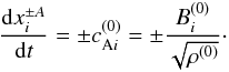 (13)The ray position
x±A = x±A(t)
is the position of a point on a wavefront at time t. Then, Eq. (13) indicates that each point on a wavefront of
an Alfvénic perturbation propagates along the background magnetic field at the local Alfvén
velocity. When
(13)The ray position
x±A = x±A(t)
is the position of a point on a wavefront at time t. Then, Eq. (13) indicates that each point on a wavefront of
an Alfvénic perturbation propagates along the background magnetic field at the local Alfvén
velocity. When  is
inhomogeneous, different parts of a wavefront propagate at different speeds. Thus, plane
wavefronts are bent and distorted, and increasingly smaller scales are generated in the
perturbation. The wavevector k±A
varies along the rays according to the equation
is
inhomogeneous, different parts of a wavefront propagate at different speeds. Thus, plane
wavefronts are bent and distorted, and increasingly smaller scales are generated in the
perturbation. The wavevector k±A
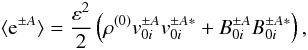
varies along the rays according to the equation 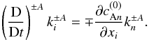 (14)The energy density (energy
per unit volume) associated with perturbations can be decomposed as a sum of contributions
due to different propagating modes. The dimensionless energy density of Alfvén waves
(normalized to
(14)The energy density (energy
per unit volume) associated with perturbations can be decomposed as a sum of contributions
due to different propagating modes. The dimensionless energy density of Alfvén waves
(normalized to  ) is given by
 where the asterisc
indicates complex conjugate and angular brackets indicate an average of fast variations
associated with the shortest scale δ. Thus,
⟨ e±A ⟩ varies on the spatial scale
l0 of the equilibrium. At the order
δ0 of the expansion, the evolution equation for the energy
density ⟨ e±A ⟩ of Alfvénic perturbations is derived:
where the asterisc
indicates complex conjugate and angular brackets indicate an average of fast variations
associated with the shortest scale δ. Thus,
⟨ e±A ⟩ varies on the spatial scale
l0 of the equilibrium. At the order
δ0 of the expansion, the evolution equation for the energy
density ⟨ e±A ⟩ of Alfvénic perturbations is derived:
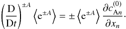 (15)This equation indicates
that, in the ideal case considered here, variations in the energy density along the rays are
due to the divergence of the vector field .
Equations (12)−(15) give a “Lagrangian” description of the
evolution of Alfvénic perturbations along magnetic lines. They will be used to describe the
evolution of Alfvénic perturbations in a complex 3D magnetic structure that models the
magnetic field of a coronal hole.
(15)This equation indicates
that, in the ideal case considered here, variations in the energy density along the rays are
due to the divergence of the vector field .
Equations (12)−(15) give a “Lagrangian” description of the
evolution of Alfvénic perturbations along magnetic lines. They will be used to describe the
evolution of Alfvénic perturbations in a complex 3D magnetic structure that models the
magnetic field of a coronal hole.
3. Equilibrium structure
To solve the set of Eqs. (12)−(15), a form of the equilibrium quantities ρ(0)(x), B(0)(x) must be specified, which represents a model for the equilibrium structure of a coronal hole. The magnetic field in a coronal hole is characterized by a dominant polarity. However, magnetograms in coronal holes (Zhang et al. 2006) show that several regions are present where the photospheric magnetic field has the polarity opposite to the dominant one. Areas of the two polarities appear to be intermixed, forming a complex structure where different spatial scales are present, ranging from ~109 cm down to the resolution limit. The area corresponding to magnetic flux with the dominant polarity represents ~70% of the total area, the remaining 30% being due to the opposite polarity (Zhang et al. 2006). The coronal magnetic field above such regions should have a complex structure as well: closed magnetic lines connecting regions of opposite polarity should be present, along with open magnetic lines emanating from dominant polarity regions. At sufficiently high altitudes, only open magnetic lines should be found, and the structure of the magnetic field is less complex. A picture of the whole magnetic structure can be found in Zhang et al. (2006).
We built up a model for the coronal magnetic field that tries to take the above-described features into account through a number of assumptions:
-
(i)
We represent a relatively small portion of the corona neglecting curvature effects due to the spherical geometry. Then, we use a Cartesian reference frame where the xy plane corresponds to the coronal base, while the z axis is vertically upward directed. The spatial domain is D = { (x,y,z) } = [0,l] × [0,l] × [0, + ∞). The size of the base square is l = 1 in dimensionless units, and it corresponds to the length L used to normalize the spatial coordinates.
-
(ii)
At the coronal base z = 0, the magnetic field B(0) has a complex structure; the effects of these boundary conditions at z = 0 become less relevant with increasing the altitude z, and the structure of B(0) becomes simpler at larger z. We assume that B(0) becomes uniform and directed in the vertical z direction in the limit z → + ∞. This can be represented by writing the equilibrium magnetic field in the following form:
 (16)where the first
term on the R.H.S. is a uniform field,
ez being the unit vector
directed in the vertical z direction, while the second term is a
nonuniform field such that
(16)where the first
term on the R.H.S. is a uniform field,
ez being the unit vector
directed in the vertical z direction, while the second term is a
nonuniform field such that  (17)
(17) -
(iii)
The equilibrium magnetic field B(0) satisfies the force-free condition ∇ × B(0) = αB(0). This condition is a natural requirement, since it is satisfied well by an equilibrium magnetic field in a low-β plasma, like the coronal plasma. The scalar quantity α is constant along fieldlines. For large values of z the magnetic field B(0) is almost uniform (Eq. (17)), corresponding to α ≃ 0. This value of α propagates down to lower altitudes along fieldlines. Then, the simplest way to represent this situation is to assume that α = 0 in the whole domain D, i.e., to take B(0) as a current-free field.
 (18)This assumption is
probably not critical. Indeed, we show that the main results are essentially
independent of the details of the equilibrium field. Equation (18) implies that the inhomogeneous
component B1(x)
can be expressed in terms of a scalar potential Φ(x):
(18)This assumption is
probably not critical. Indeed, we show that the main results are essentially
independent of the details of the equilibrium field. Equation (18) implies that the inhomogeneous
component B1(x)
can be expressed in terms of a scalar potential Φ(x):
 (19)The divergenceless
condition ∇·B1 = 0 gives the Laplace equation
for the scalar potential:
(19)The divergenceless
condition ∇·B1 = 0 gives the Laplace equation
for the scalar potential:  (20)
(20) -
(iv)
Magnetograms in coronal holes reveal a statistically homogeneous structure, where regions of the two polarities appear to be randomly distributed and no dominant structures are present (Zhang et al. 2006). We represent this situation assuming that Φ(x) at the base z = 0 varies in x and y on a typical scale length l0 and that it is periodic along x and y on the whole domain D. Statistical homogeneity is represented well provided that l0 is sufficiently smaller than the unitary periodicity length (Pommois et al. 1998). The periodicity condition allows us to expand the potential Φ in Fourier series in the x and y variables:
 (21)where
nx and
ny are integers, and
i is the imaginary unit. Inserting this expression into the Laplace
Eq. (20) we derive the equation for
the Fourier amplitude φ of the potential
(21)where
nx and
ny are integers, and
i is the imaginary unit. Inserting this expression into the Laplace
Eq. (20) we derive the equation for
the Fourier amplitude φ of the potential  (22)where
 is the horizontal wavenumber (not necessarily integer). The only solution of
Eq. (22) that satisfies the
condition (17) is a decaying
exponential in the form
is the horizontal wavenumber (not necessarily integer). The only solution of
Eq. (22) that satisfies the
condition (17) is a decaying
exponential in the form  (23)where
A(nx,ny)
are complex coefficients that are determined by the boundary conditions at
z = 0. We assume that the horizontal wavenumber n
varies in the range
nmin ≤ n ≤ nmax.
Then, the largest and smallest horizontal lengths (in normalized units) in the
magnetic field structure are given by
lmax = 1/nmin and
lmin = 1/nmax, respectively.
Using Eq. (23), we write the
components of the magnetic field B1 in the
form:
(23)where
A(nx,ny)
are complex coefficients that are determined by the boundary conditions at
z = 0. We assume that the horizontal wavenumber n
varies in the range
nmin ≤ n ≤ nmax.
Then, the largest and smallest horizontal lengths (in normalized units) in the
magnetic field structure are given by
lmax = 1/nmin and
lmin = 1/nmax, respectively.
Using Eq. (23), we write the
components of the magnetic field B1 in the
form: ![Mathematical equation: \begin{eqnarray} \label{B1x} B_{1x}(\vec{x})&=&2\pi {\rm i}\! \sum_{n=n_{\min}}^{n_{\max}} \!n_x A(n_x,n_y) \exp \lbrace 2\pi \lbrack {\rm i}(n_x x + n_y y)\! -\!nz\rbrack\rbrace \\[0.1mm] \label{B1y} B_{1y}(\vec{x})&=&2\pi {\rm i}\! \sum_{n=n_{\min}}^{n_{\max}}\! n_y A(n_x,n_y) \exp \lbrace 2\pi \lbrack {\rm i}(n_x x + n_y y) \!-\!nz\rbrack\rbrace \\[0.1mm] \label{B1z} B_{1z}(\vec{x})&=&-2\pi\! \sum_{n=n_{\min}}^{n_{\max}}\! n A(n_x,n_y) \exp \lbrace 2\pi \lbrack {\rm i}(n_x x + n_y y)\! -\!nz\rbrack\rbrace . \end{eqnarray}](/articles/aa/full_html/2013/01/aa19307-12/aa19307-12-eq118.png) We
write the complex coefficients
A(nx,ny)
in terms of their modules and phases
γ(nx,ny):
We
write the complex coefficients
A(nx,ny)
in terms of their modules and phases
γ(nx,ny):
 The reality condition
of the potential Φ(x) implies that
The reality condition
of the potential Φ(x) implies that  (27)Using Eqs. (27), after some algebra, the equilibrium
magnetic field components are written in the following forms, which contain only real
quantities:
(27)Using Eqs. (27), after some algebra, the equilibrium
magnetic field components are written in the following forms, which contain only real
quantities: ![Mathematical equation: \begin{eqnarray} \label{B0x} B_x^{(0)}(\vec{x}) &=& \sum_{n_{\min} \le n \le n_{\max},\, n_x>0} \frac{n_x}{n} b(n_x,n_y) \nonumber \\[0.9mm] &&\times \, \sin \lbrack 2\pi (n_x x + n_y y) + \gamma (n_x,n_y)\rbrack \exp (-2\pi nz) \\[0.9mm] \label{B0y} B_y^{(0)}(\vec{x}) &=& \sum_{n_{\min} \le n \le n_{\max}, \, n_y>0} \frac{n_y}{n} b(n_x,n_y) \nonumber \\[0.9mm] &&\times \, \sin \lbrack 2\pi (n_x x + n_y y) + \gamma (n_x,n_y)\rbrack \exp (-2\pi nz) \\[0.9mm] \label{B0z} B_z^{(0)}(\vec{x}) &=& B_0 + \left( \sum_{n_{\min} \le n \le n_{\max},\, n_x>0} + \sum_{n_x=0,0 < n_y \le n_{\max}} \right) b(n_x,n_y) \nonumber \\[0.9mm] &&\times \, \cos \lbrack 2\pi (n_x x + n_y y) + \gamma (n_x,n_y)\rbrack \exp (-2\pi nz) \end{eqnarray}](/articles/aa/full_html/2013/01/aa19307-12/aa19307-12-eq122.png)
where
b(nx,ny) = −4πn|A(nx,ny)|.
The above expressions indicate that B1 is given by
a superposition of terms: each term varies on a horizontal scale
l = 1/n and exponentially decays with
the altitude z on the scale height 2πl. Then, at high
enough altitudes the inhomogeneous component B1 is
negligible and the equilibrium magnetic field B(0)
reduces to a homogeneous vertical field given by
B0ez.
Moreover, the spatial average of the inhomogeneus component is vanishing at any given
altitude:  . Then,
B0ez
represents the average field, corresponding to the dominant polarity.
. Then,
B0ez
represents the average field, corresponding to the dominant polarity.
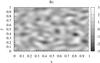 |
Fig. 1 Vertical component |
Equations (28)–(30) contain some parameters that need to be specified
-
a)
Since no anisotropy is present in the horizontal directions, the amplitudes b(nx,ny) only depend on the wavenumber n. Moreover, we assume that this dependence follows a power law:
 (31)where
c and μ are a normalization constant and the
spectral index, respectively. Equation (31) expresses the idea that the magnetic field structure is the result of a
turbulent process taking place beneath the coronal base. For instance, the value
μ = 4/3 is the index of the amplitude spectrum associated with a 2D
Kolmogorov energy spectrum (Malara et al. 2005). In the present model μ represents a free parameter
that has been chosen in a range between 1/2 and 4/3. The normalization constant
c is such that
(31)where
c and μ are a normalization constant and the
spectral index, respectively. Equation (31) expresses the idea that the magnetic field structure is the result of a
turbulent process taking place beneath the coronal base. For instance, the value
μ = 4/3 is the index of the amplitude spectrum associated with a 2D
Kolmogorov energy spectrum (Malara et al. 2005). In the present model μ represents a free parameter
that has been chosen in a range between 1/2 and 4/3. The normalization constant
c is such that  .
. -
b)
Due to the form (31), the maximum amplitude is on the largest spatial scale lmax, corresponding to the typical scale l0 of the equilibrium structure. As discussed above, in order to reproduce statistical homogeneity we used l0 ~ lmax = 1/4, corresponding to nmin = 4. The value of maximum wavenumber ranges between nmax = 10 and nmax = 15. With this choice each component of B1 is a superposition of few hundreds of harmonics, which gives a complex magnetic structure but computational times not exceedingly long.
-
c)
The parameter B0 gives the amplitude of the homogeneous component, which corresponds to the dominant polarity. We used a value of B0 such that at z = 0 the area where
 (representing the dominant
polarity) is ~ 70% of the total area (Zhang et al. 2006).
(representing the dominant
polarity) is ~ 70% of the total area (Zhang et al. 2006). -
d)
Since B(0) does not represent any particular magnetic field, the phases γ(nx,ny) have been randomly chosen in the interval [0,2π] .
In Fig. 1 the vertical component
 is plotted as a function of the
x and y normalized coordinates at the base
z = 0 of the spatial domain, for
μ = 4/3. It can be seen that the distribution of the
magnetic field is statistically homogeneous with no large-scale structure. The positive
polarity is dominant but several areas of the opposite polarity are also present. These
features are reminiscent of magnetograms taken in coronal hole regions (Zhang et al. 2006).
is plotted as a function of the
x and y normalized coordinates at the base
z = 0 of the spatial domain, for
μ = 4/3. It can be seen that the distribution of the
magnetic field is statistically homogeneous with no large-scale structure. The positive
polarity is dominant but several areas of the opposite polarity are also present. These
features are reminiscent of magnetograms taken in coronal hole regions (Zhang et al. 2006).
A picture of the 3D structure of the equilibrium magnetic field B(0) can be obtained by plotting magnetic lines that are represented in Fig. 2, in the case μ = 4/3. It can be seen that the magnetic field has a complex structure where both open and closed fieldlines are present. Closed magnetic lines are in the form of small arches connecting regions of opposite polarity at the base. These arches are confined at low altitudes, most of them remaining below z ~ 0.02 (in normalized units). Open field lines have an arbitrary orientation at low altitudes but tend to become vertically oriented with increasing z.
We expect that the magnetic structure contains several separatrices. For instance, separatrices are surfaces that separate adjacent regions of open or closed fieldlines. Moreover, open fieldlines coming from distant regions at the base converge on the two sides of a separatrix at high altitudes (see Sect. 4.3). Since Alfvénic perturbations propagate along magnetic lines, at separatrices the perturbation pattern is strongly stretched. Malara et al. (2007) have shown that the rate of small-scale generation is particularly high at such locations. We will show that small-scale structures in the perturbation are located at separatrices.
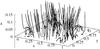 |
Fig. 2 Magnetic lines of the equilibrium magnetic field B(0), for μ = 4/3. |
Concerning the equilibrium density, we adopted the simplest choice by assuming that
ρ(0) is uniform. In this case, the divergenceless condition
for the equilibrium magnetic field B(0) implies
that  . Then, Eq. (15) reduces to
 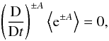 (32)indicating that the
energy density of Alfvénic perturbations remains constant along magnetic lines.
(32)indicating that the
energy density of Alfvénic perturbations remains constant along magnetic lines.
4. Alfvén wave evolution
We study the evolution of an Alfvénic perturbation propagating in the magnetic structure described in the previous section. This perturbation enters the domain D through the base z = 0, propagates upwards to cross the inhomogeneous region at low altitudes, and finally reaches the upper part of D where the magnetic field is essentially homogeneous and vertically directed. In particular, we are interested in describing the evolution of the wavevector k±A, which is modified when the perturbation goes across the inhomogeneous region. For simplicity, we consider the evolution of an initially monochromatic wave with a given amplitude, and this corresponds to the assumption that both the wavevector k±A and the energy density ⟨ e±A ⟩ are uniform at the z = 0 plane. In that case, Eq. (32) implies that the energy density of the perturbation is uniform in the whole domain D. The evolution of k±A along the rays is described by Eq. (14), while Eq. (13) determines the ray trajectories, which coincide with magnetic lines of B(0). Since the dominant polarity of B(0) in our model is positive, we consider a perturbation that propagates in the same direction as B(0). This corresponds to taking only the upper sign in Eqs. (13) and (14). In points of the base z = 0 where B(0) is negative (polarity opposite to the dominant one), this perturbation would propagate downward, and it would not enter the domain. Then, we consider only rays that start from areas at the base where B(0) > 0.
A detailed description of the perturbation evolution can be obtained by solving Eqs. (13) and (14) for a large number of rays that fill the base area as uniformly as possible.
For this reason we considered the evolution of N = 30 000 rays whose
starting points are randomly chosen at z = 0. Integrating Eqs. (13) and (14) corresponds to moving along each magnetic line with a nonuniform Alfvén speed
 .
Then, a constant integration step Δt would give nonconstant steps along the
magnetic line. This can be avoided by performing a change of variable, from time
t to the space
s = s(t) measured along a given magnetic
line. These quantities are related by
.
Then, a constant integration step Δt would give nonconstant steps along the
magnetic line. This can be avoided by performing a change of variable, from time
t to the space
s = s(t) measured along a given magnetic
line. These quantities are related by  .
Using the new variable s, Eqs. (13) and (14) are rewritten in the
form:
.
Using the new variable s, Eqs. (13) and (14) are rewritten in the
form: 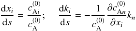 (33)where
the upper index “+A” in the quantities
xi and
ki has been dropped to simplify the
notation. Equations (33) have been
numerically solved using a fourth-order Runge-Kutta scheme, for each of the
N rays describing the whole perturbation. As discussed above, the initial
position of each ray is randomly chosen at the base z = 0, while the
initial wavevector is the same for all the rays:
k(s = 0) = k0 = (k0x,k0y,k0z).
In particular, we used the values
k0x = k0y = k0z = 20π/l0,
in order to fulfil the condition λ ≪ l0.
(33)where
the upper index “+A” in the quantities
xi and
ki has been dropped to simplify the
notation. Equations (33) have been
numerically solved using a fourth-order Runge-Kutta scheme, for each of the
N rays describing the whole perturbation. As discussed above, the initial
position of each ray is randomly chosen at the base z = 0, while the
initial wavevector is the same for all the rays:
k(s = 0) = k0 = (k0x,k0y,k0z).
In particular, we used the values
k0x = k0y = k0z = 20π/l0,
in order to fulfil the condition λ ≪ l0.
For each ray, Eqs. (33) are integrated until one of the two following conditions has been fulfiled:
-
(a)
the vertical coordinate z becomes larger than zh = 0.25. In this case, the ray trajectory coincides with an open fieldline; for z ≥ zh, this ray has reached the region where B(0) is homogeneous, after crossing the low-altitude inhomogeneous region.
-
(b)
The vertical coordinate z becomes negative. In this case the ray has moved along a closed fieldline, finally coming back to the base of the domain D in a negative polarity area.
Since we are interested in studying the perturbation that reaches the high-altitude homogeneous region, only rays satisfying condition (a) have been retained. We indicate the number of rays satisfying condition (a) by Nopen. The area of the base surface at z = 0 where open fieldlines are emanated from is indicated by Sopen.
4.1. Small-scale formation in the perturbation
We collected the values of the wavevector k associated with each ray satisfying condition (a) at the altitude z = zh. Such values k(z = zh) are in general different from the initial value k0. In some case we found k(z = zh) to be much larger than k0: increases in k correspond to the formation of small scales. The values k(z = zh) turn out to be continuosly distributed, thus forming a spectrum.
The energy spectrum of the perturbation in the region of homogeneous magnetic field can
be calculated by the following procedure. The whole perturbation can be decomposed into
small packets. Each packet is labelled by the index α; it has a small
volume δVα, and it
propagates along a ray carrying an energy
δEα = ⟨ e ⟩ δVα.
When dissipation can be neglected, as in the present case, energy
δEα remains constant
during the packet propagation (Malara et al. 2003).
We select a volume V in the region of homogeneous magnetic field
(z ≥ zh) in the form of a parallelepiped:
the base of V is equal to the base S of the whole domain
D. When packets reach the volume V their wavevector
kα does not change any more, since
B(0) is uniform in V. We can
group such packets according to the value of
kα: we divide the k axis
into a sequence of adjacent bins I(k), and each bin has
amplitude Δk and is centred on a value k. Then, for each
bin we sum the energy of all packets whose wavevector falls into the bin itself. This
energy is indicated by 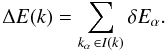 (34)The energy
spectrum per unit volume is defined as
ϵ(k) = ΔE(k)/(V Δk).
In Appendix A we show that the energy spectrum in the homogeneous region can be written in
the form
(34)The energy
spectrum per unit volume is defined as
ϵ(k) = ΔE(k)/(V Δk).
In Appendix A we show that the energy spectrum in the homogeneous region can be written in
the form  (35)where
  (36)with
kz.α the
z-component of
kα (parallel to
B(0)). In the present case
⟨ e ⟩ is constant, while
Sopen/S ≃ 0.5 for all
the considered equilibrium configurations.
(36)with
kz.α the
z-component of
kα (parallel to
B(0)). In the present case
⟨ e ⟩ is constant, while
Sopen/S ≃ 0.5 for all
the considered equilibrium configurations.
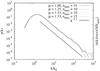 |
Fig. 3 Distribution p(k) as a function of the normalized wavevector k/k0, calculated for different values of the parameters μ and nmax of the equilibrium magnetic field B(0). The quantity p(k) is proportional to the fluctuation spectrum per unit volume ϵ(k) in the homogeneous region. A power law with slope −α = −2.3 is also shown for comparison. |
The distribution p(k), which is proportional to the energy spectrum ϵ(k), has been calculated from the solution of Eqs. (33). In Fig. 3 we plotted the wavevector distribution p(k) calculated for different values of the slope μ and of the maximum wavenumber nmax in the equilibrium magnetic field spectrum (Eq. (31)). Wavevector values are normalized to the initial value k0 at the base z = 0. We see that the initially monochromatic spectrum is modified when the perturbation crosses the inhomogeneous region: though the maximum energy is still at k ≃ k0, part of the energy has been trasferred at larger wavevectors, forming a power-law tail. We note that the form of ϵ(k) is essentially independent of the parameters μ and nmax. Thus, the perturbation spectrum that is generated in the inhomogeneous region has a form that does not depend on the details of the inhomogeneous equilibrium magnetic field B(0). A fit in the power-law range (see Fig. 3) shows that ϵ(k) ∝ k−α, with α ≃ 2.3. We note that the spectral index α is larger than both the Kolmogorov (5/3) and the Kraichnan (3/2) value. Then, the interaction of the Alfvénic perturbation with the inhomogeneous magnetic field generates a spectrum that is steeper than what would be formed by nonlinear interactions in a turbulence.
From Fig. 3 it is seen that the power law extends down to a cutoff corresponding to the largest wavevector kmax. We find that the extension of the spectrum increases with increasing the number N of the considered rays. If one assumes that kmax → ∞ for N → ∞, then it follows that the magnetic structure contains locations where infinitesimally small scales are generated in the perturbation pattern. At these locations, singularities are formed. Of course, if dissipative effects (neglected in the present approach) were included, then the power-law range would have an upper limit corresponding to the dissipative range.
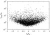 |
Fig. 4 Scatter plot with the values k||/k0 and k⊥/k0 displayed on the horizontal and vertical axes, respectively. These values are calculated for N = 10 000 rays at z = zh, in the case μ = 1.33, nmax = 10. |
Considering the population of wavevectors k at
z = zh, the components of each wavevector
parallel and perpendicular to the local magnetic field
B(0) has been calculated. These are defined by
 A scatter plot is shown
in Fig. 4, with the values of
k|| and k⊥ for all the
rays at z = zh. It can be seen that
k⊥ reaches values much higher than
|k|||. The energy spectrum of perturbation is
anisotropic, and it has an extension in the directions perpendicular to the magnetic field
B(0) larger than in the parallel direction.
The structures on the smallest scales have a wavevector that is nearly perpendicular to
B(0). This kind of anisotropy is
qualitatively similar to what is found in MHD turbulence, where the nonlinear energy
cascade tends to take place in the directions perpendicular to the background magnetic
field (e.g., Shebalin et al. 1983; Carbone
& Veltri 1990). However, in the present
model nonlinear effects have been completely neglected: the anisotropy in the fluctuation
spectrum is only due to the linear interaction between Alfvénic fluctuations and the
inhomogeneous background.
A scatter plot is shown
in Fig. 4, with the values of
k|| and k⊥ for all the
rays at z = zh. It can be seen that
k⊥ reaches values much higher than
|k|||. The energy spectrum of perturbation is
anisotropic, and it has an extension in the directions perpendicular to the magnetic field
B(0) larger than in the parallel direction.
The structures on the smallest scales have a wavevector that is nearly perpendicular to
B(0). This kind of anisotropy is
qualitatively similar to what is found in MHD turbulence, where the nonlinear energy
cascade tends to take place in the directions perpendicular to the background magnetic
field (e.g., Shebalin et al. 1983; Carbone
& Veltri 1990). However, in the present
model nonlinear effects have been completely neglected: the anisotropy in the fluctuation
spectrum is only due to the linear interaction between Alfvénic fluctuations and the
inhomogeneous background.
4.2. Small-scale structures
The small scales generated in the Alfvénic perturbation have a coherent spatial structure. To visualize how small scales are spatially distributed, we first selected the rays whose wavevector k at the altitude zh is larger than a threshould value, given by kthr = 4k0. This subset of wavevectors is located inside the power-law range of the distribution (see Fig. 3). Each of these k vectors has been projected onto the xy plane, thus obtaining the horizontal wavevectors kho = (kx,ky,0). Since at z = zh the magnetic field B(0) is nearly vertical, then kho is nearly perpendicular to B(0), and then it represents the main component of k. Finally, we normalized each horizontal wavevector, obtaining a set of unit vectors K = kho/kho. Thus, the unit vectors K give the directions of the wavectors k in large-scale structures, projected on the horizontal plane.
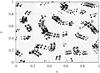 |
Fig. 5 Unit vectors K (arrows) giving the direction of wavevectors k of large-scale structures, at z = zh, projected on the horizontal xy plane. The starting points of each unit vector (large square dots) are the (x,y) positions of the corresponding rays at z = zh. The dotted area represents the area at the base z = 0 where Bz ≥ 0. The segment AB is also plotted. |
In Fig. 5 we plotted all the unit vectors K; the starting points of each vector K are taken at the (x,y) positions of the corresponding rays. Thus, Fig. 5 illustrates both the spatial location of small-scale structures and the local orientation of the corresponding wavevector. In Fig. 5 small scales appear to be structured as curved lines. These lines are at altitude z = zh; however, at higher altitutes wavevectors do not evolve any more and rays are parallel to the z direction. Then, the pattern of Fig. 5 representing small-scale structures remains essentially unchanged, thereby increasing z. This implies that small-scale structures are distributed along sheets that are elongated in the direction parallel to the magnetic field B(0). The linear structures in Fig. 5 are the intersections between these sheets and the horizontal plane z = zh. The perturbation wavevector k is locally quasi-perpendicular to the sheet surface.
From Fig. 5 it can be seen that small-scale structures (at z ≥ zh) are essentially located above regions of negative magnetic polarity. We show that this property is related to the topology of magnetic lines around those opposite polarity regions. We observed that increasing the threshold wavevector kthr does not substantially modify the results shown in Fig. 5.
4.3. Discontinuities
To obtain a more detailed description of small-scale structures we calculated how the
wavevector k varies across one of these structures. In particular, we
selected a horizontal segment, denoted by AB, that crosses one particular small-scale
structure at altitude z = zh, and we
calculated the profile of k along such a segment. The segment AB is drawn
in Figs. 5 and 6; the endpoints have coordinates
A = (xA,yA,zh) = (0.8,0.57,0.25)
and
B = (xB,yB,zh) = (0.9,0.67,0.25).
We followed the following procedure. First, we defined a uniform grid of
Np + 1 points
{ Xn = (xn,yn,zn) }
located on the segment AB:  (37)with
Δx = (xB − xA)/Np,
Δy = (yB − yA)/Np,
and Np = 1000.
(37)with
Δx = (xB − xA)/Np,
Δy = (yB − yA)/Np,
and Np = 1000.
Second, magnetic lines are used to define a mapping
Γ: X → X′ between points at the altitude
z = zh and points at the base
z = 0. Each point X at
z = zh is connected to a corresponding
point X′ at z = 0 by an open magnetic line
which goes from X′ to X. In particular, we
calculated a set of Np + 1 magnetic lines: the
nth magnetic line starts at the gridpoint
Xn on the segment AB and it is followed
downwards, until it crosses the base z = 0 at corresponding point
 . The points
 are located
along a curved line A′B′ at z = 0 which represents
the map of the segment AB on the base z = 0. The segment AB, the line
A′B′, and some magnetic lines defining the mapping Γ are
represented in Fig. 6. It can be seen that Γ is a
discontinuous mapping: the continuous segment AB is mapped into a discontinuous curve
A′B′. This is because the curve A′B′ needs
to be located in regions of open fieldlines, while magnetic lines crossing the segment AB
come from two separated open fieldline regions (Fig. 6). Two distinct magnetic lines
are located
along a curved line A′B′ at z = 0 which represents
the map of the segment AB on the base z = 0. The segment AB, the line
A′B′, and some magnetic lines defining the mapping Γ are
represented in Fig. 6. It can be seen that Γ is a
discontinuous mapping: the continuous segment AB is mapped into a discontinuous curve
A′B′. This is because the curve A′B′ needs
to be located in regions of open fieldlines, while magnetic lines crossing the segment AB
come from two separated open fieldline regions (Fig. 6). Two distinct magnetic lines  and
and
 coming from two
distant regions at the base z = 0 converge towards the point C on the
segment AB, approaching each other (see Fig. 6). The
“singular” point C is the point where the mapping Γ is discontinuous, and it represents
the intersection between the segment AB and a separatrix surface. Magnetic lines on the
two sides of such a separatrix are connected to the two positive polarity areas at the
base z = 0.
coming from two
distant regions at the base z = 0 converge towards the point C on the
segment AB, approaching each other (see Fig. 6). The
“singular” point C is the point where the mapping Γ is discontinuous, and it represents
the intersection between the segment AB and a separatrix surface. Magnetic lines on the
two sides of such a separatrix are connected to the two positive polarity areas at the
base z = 0.
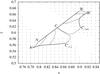 |
Fig. 6 Segment AB (straight full line), the two portions
|


Third, the set of Eqs. (33) are solved
along the Np + 1 magnetic lines defined above. The initial
position x(s = 0) of each ray is one of the
points  along the
curve A′B′, while the initial wavevector is
k(s = 0) = (k0x,k0y,k0z)
for all the rays. Equations (33) are
integrated until each ray reaches the altitude
z = zh, thus crossing the segment AB. The
final values of k thus obtained give the profile of the
wavevector along the segment AB.
along the
curve A′B′, while the initial wavevector is
k(s = 0) = (k0x,k0y,k0z)
for all the rays. Equations (33) are
integrated until each ray reaches the altitude
z = zh, thus crossing the segment AB. The
final values of k thus obtained give the profile of the
wavevector along the segment AB.
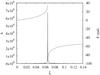 |
Fig. 7 Wavevector k (full line) and the phase function F (dashed line) as functions of the coordinate ξ along the segment AB. |
To represent such a profile it is useful to introduce the coordinate ξ
running along the segment AB: the value ξ = 0 corresponds to the point A;
ξ = lAB corresponds to the point B
( being the length of AB); while
ξC ≃ 0.0656 correspond to the singular point C. The
dependence of k on the coordinate ξ is shown in
Fig. 7. It can be seen that the
wavevector k diverges to infinity at the singular point
ξ = ξC
being the length of AB); while
ξC ≃ 0.0656 correspond to the singular point C. The
dependence of k on the coordinate ξ is shown in
Fig. 7. It can be seen that the
wavevector k diverges to infinity at the singular point
ξ = ξC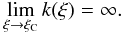 (38)Thus, small-scale
structures contain locations where the wavevector grows locally without limit.
(38)Thus, small-scale
structures contain locations where the wavevector grows locally without limit.
From the knowledge of the function k(ξ),
the dependence of the phase function F on the coordinate
ξ can be derived in the following way. The unit vector
 gives
the direction of the segment AB. We take the dot product of Eq. (9) with u to
obtain the directional derivative
dF/dξ of the phase function along
the segment AB:
gives
the direction of the segment AB. We take the dot product of Eq. (9) with u to
obtain the directional derivative
dF/dξ of the phase function along
the segment AB:  (39)This equation
holds for any value of ξ except ξC where
k diverges. Then it can be integrated over any interval
[ξ0,ξ] that does not contain
ξC:
(39)This equation
holds for any value of ξ except ξC where
k diverges. Then it can be integrated over any interval
[ξ0,ξ] that does not contain
ξC:  (40)where
F0 is the value of F at the point
ξ0.
(40)where
F0 is the value of F at the point
ξ0.
Since k(ξ) diverges at singular point ξ = ξC, the phase function F(ξ) could diverge for ξ → ξC. To clarify this point, we studied the behaviour of k(ξ) in more detail in the vicinity of point ξC. In Fig. 8 the wavevector component k·u is plotted as a function of |ξ − ξC| on both sides of the singular point ξC. It can be seen that (k·u) ∝ |ξ − ξC|−β for ξ → ξC, with β ≃ 0.85. Since β < 1 it follows that the integral in Eq. (40) does not diverge in the limit ξ → ξC. Thus, the phase function F(ξ) remains finite at the singular point ξC.
Another property of the phase function is that F(ξ) is
discontinuous at ξC. In fact, according to Eq. (12) F propagates along
magnetic lines at the local Alfvén speed. Magnetic lines
and
converge at the
singular point coming from distant parts (Fig. 6);
thus, the values of F on the two sides of ξC
at any given time t are, in general, different. This produces a jump
ΔF in the phase across the singular point. The jump ΔF
can be calculated in the following way. The phase function F has a simple
expression at the base z = 0 where the wave has a given wavevector
k0:  (41)with
 . We can arbitrarily choose the
time origin; then, we set t = 0 as the time when two rays travelling
along magnetic lines and
simultaneously
reach the singular point C. We indicate by Δt(−) and
Δt(+ ) the time intervals that these two rays take to
travel along the magnetic lines and
, respectively. The
times Δt(−) and Δt(+ ) have
been calculated by integrating Eq. (13)
along such magnetic lines. We indicate by F(−) and
F(+ ) the values of the phase on the two sides of the
singular point C at time t = 0. Since the phase remains constant in the
space-time along each ray, using the expression (41) we find
. We can arbitrarily choose the
time origin; then, we set t = 0 as the time when two rays travelling
along magnetic lines and
simultaneously
reach the singular point C. We indicate by Δt(−) and
Δt(+ ) the time intervals that these two rays take to
travel along the magnetic lines and
, respectively. The
times Δt(−) and Δt(+ ) have
been calculated by integrating Eq. (13)
along such magnetic lines. We indicate by F(−) and
F(+ ) the values of the phase on the two sides of the
singular point C at time t = 0. Since the phase remains constant in the
space-time along each ray, using the expression (41) we find 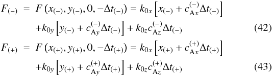 where
we used the notation
where
we used the notation  ,
,
 ,
,
 , and
, and
 . Then, the jump in the phase
function at the singular point has been calculated as
ΔF = F(+ ) − F(−).
Finally, using Eq. (40) and the above
value for the jump ΔF at the singular point, the phase function
F(ξ) along the segment AB has been calculated. The
discontinuous profile of F(ξ) is plotted in Fig. 7. The discontinuity in the phase function corresponds to
a discontinuity in the perturbation quantities: velocity
v+A and magnetic field
B+A.
. Then, the jump in the phase
function at the singular point has been calculated as
ΔF = F(+ ) − F(−).
Finally, using Eq. (40) and the above
value for the jump ΔF at the singular point, the phase function
F(ξ) along the segment AB has been calculated. The
discontinuous profile of F(ξ) is plotted in Fig. 7. The discontinuity in the phase function corresponds to
a discontinuity in the perturbation quantities: velocity
v+A and magnetic field
B+A.
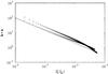 |
Fig. 8 Wavevector component k·u as a function of |ξ − ξC| for ξ < ξC (crosses) and for ξ > ξC (circles). A function proportional to |ξ − ξC|-0.85 (full line) is plotted for comparison. |
Summarizing, the small-scale structure under consideration contains a discontinuity, which is localized on the separatrix crossed by the segment AB (Fig. 5). A similar analysis has been carried out on other small-scale structures displayed in Fig. 5, finding similar behaviour. We conclude that in many cases small-scale structures that form in the Alfvénic perturbation contain a discontinuity, where velocity and magnetic perturbations present an abrupt variation.
Finally, we point out two properties of small-scale structures: (i) the wavevector
k is quasi-perpendicular to the background magnetic
field B(0); (ii) the total magnetic field
intensity (equilibrium field + perturbation) is given by ![Mathematical equation: \begin{equation} \label{Bint} B=\left\lbrack \left(B^{(0)}\right)^2 \!+\! 2 \vec{B}^{(0)}\cdot \vec{B}^{+A} \!+\! (B^{+A})^2\right\rbrack^{1/2}\! \simeq\! B^{(0)} \left[ 1\!+\! \frac{(B^{+A})^2}{2(B^{(0)})^2}\right] \end{equation}](/articles/aa/full_html/2013/01/aa19307-12/aa19307-12-eq295.png) (44)where
we used the properties that the magnetic perturbation has a small amplitude
B + A ≪ B(0),
and is polarized perpendicular to B(0). Since
B(0) is continuous, the relative jump in the
total magnetic field intensity across the discontinuity is
(44)where
we used the properties that the magnetic perturbation has a small amplitude
B + A ≪ B(0),
and is polarized perpendicular to B(0). Since
B(0) is continuous, the relative jump in the
total magnetic field intensity across the discontinuity is 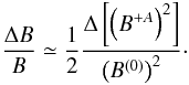 (45)Equation (45) indicates that
ΔB/B is a small quantity, of the
second order in the ratio
B±A/B(0).
The above properties (i) and (ii) imply that the discontinuities found in the present
model should be classified as either discontinuities, following the
terminology used for solar-wind DDs. Since the wavevector k
has a small but nonvanishing component along
B(0), these structures are not static TDs. On the
contrary, they are RDs propagating away from the Sun along the background magnetic field,
with k forming large angles with
B(0).
(45)Equation (45) indicates that
ΔB/B is a small quantity, of the
second order in the ratio
B±A/B(0).
The above properties (i) and (ii) imply that the discontinuities found in the present
model should be classified as either discontinuities, following the
terminology used for solar-wind DDs. Since the wavevector k
has a small but nonvanishing component along
B(0), these structures are not static TDs. On the
contrary, they are RDs propagating away from the Sun along the background magnetic field,
with k forming large angles with
B(0).
5. Summary and discussion
In this paper we have presented a model describing the evolution of Alfvénic perturbations that propagate in open-fieldline regions of the solar corona. The model describes how perturbations propagating upward along open fieldlines are modified when they cross a region with an inhomogeneous magnetic field that should be present at low altitudes in the corona.
Magnetograms of the photospheric magnetic field in coronal holes (Zhang et al. 2006) reveal the presence of regions with magnetic polarity opposite to the dominant polarity, irregularly intermixed. We built up a 3D model for the magnetic field in a coronal hole, and this model is a potential field formed by the superposition of several harmonics on different spatial scales and a uniform vertical magnetic field. The resulting structure has a complex pattern containing both closed and open fieldlines. At high altitudes only the uniform component makes a nonnegligible contribution, corresponding to the dominant polarity of the coronal hole. By a comparison with magnetograms (Zhang et al. 2006), the horizontal characteristic length of magnetic structures can be assumed to be L0 ~ 3 × 10⁴ km, corresponding to the value L = 4 L0 ~ 1.2 × 10⁵ km for the unitary (periodicity) length of the model. The expression Lh = lhL ≃ L0 ~ 3 × 10⁴ km is the altitude above the coronal base where the background magnetic field B(0) becomes essentially uniform.
For the sake of simplicity, the background density ρ(0) has been assumed to be uniform in the whole domain. This choice has emphasized the role played by the background magnetic field in determining the evolution of perturbations. The scale height Hρ of the density in the corona can be estimated by assuming equilibrium between gravity and pressure gradient and a uniform temperature: Hρ ≃ κBT(0)/(mpg) where κB is the Boltzmann constant, mp the proton mass, g ≃ 2.74 × 104 cm s-2 the surface gravity of the Sun, and T(0) ≃ 106 K. Using these values, we find Hρ ≃ 3 × 10⁴ km, which is similar to the altitude Lh. Since the wave evolution takes place at altitudes lower than Lh ≃ Hρ, we conclude that assumption of uniform density should not severely influence the results of the model.
The amplitude of harmonics in the expression of B(0) has been assumed to depend on the wavenumber n as a power law, where the slope μ has been treated as a free parameter of the model. Though this assumption could appear to be strong, the results show that the final spectrum of the perturbation is essentially indepedent both of the value of μ and of the maximum wavenumber nmax (Fig. 3). This indicates that details of the analytical form of the background magnetic field B(0) are not relevant: probably, the final state of Alfvénic perturbations is mostly determined by topological properties of B(0), like the presence of separatrices. In fact, small scales in the perturbation are mainly generated around separatrix locations (McLaughlin et al. 2010).
Another assumption of the model is that perturbations have amplitudes that are smaller than the equilibrium quantities. Velocity perturbations in Alfvén waves observed in corona are of the order of 105 cm s-1 (Tomczyk & McIntosh 2009), while unresolved nonthermal velocities in corona are estimated to be ~3−5 × 106 cm s-1. Both these values are much lower than typical values of the Alfvén velocity (Tomczyk & McIntosh 2009). This justifies the small-amplitude assumption.
One result of the model is that Alfvénic perturbations crossing the inhomogeneity region develop small scales. In particular, an initially monochromatic perturbation (whose energy is concentrated at a well-defined wavevector k0 at the base z = 0) develops a spectrum where the energy is distributed in the wavevector space according to a power law. The formation of such a spectrum takes place at relatively low altitudes in the corona: at z = Lh ≃ 3 × 10⁴ km above the coronal base, for instance, the spectrum is completely formed. Moreover, the spectrum is anisotropic, the smallest scales being essentially at wavevectors k that are quasi-perpendicular to B(0). These two features are reminiscent of what happens in MHD turbulence, where nonlinear couplings generate power-law spectra with an energy cascade that mainly flows in the direction perpendicular to the mean magnetic field (e.g., Shebalin et al. 1983; Carbone & Veltri 1990). In the present model this anisotropy is generated by the coupling between the perturbation and the inhomogeneus background, instead of nonlinear effects. However, the slope α ≃ 2.3 of the pertubation spectrum that we find is much larger than what is typically found in turbulence (e.g., 1.5 or 1.66 for a Kraichnan or a Kolmogorov spectrum, respectively). Then, the present model cannot account for the formation of a fully developed spectrum. However, models studying the evolution of fluctuations from the corona to the solar wind or the solar wind acceleration by dissipation of wave energy should take the phenomenon we studied here into account. For instance, Verdini et al. (2009) present a model of turbulence formation in the sub-Alfvénic solar wind, where Alfvén waves on large scales are injected at the base and partially reflected by the vertical stratification. Though a turbulence spectrum forms as a consequence of nonlinear wave-wave interactions, the produced heat seems to be deposited at greater distances than what is needed to sustain the background wind. Our model suggests that upward-propagating waves start forming small scales already at very low altitudes. Such a phenomenon can decrease the altitude of heat deposition, thus leading to a better agreement between the results of the turbulence model and the background wind structure.
The main result of our model is that small scales are concentrated in spatially localized structures that in many cases contain a discontinuity. The phase function F, as well as the perturbed velocity v + A and magnetic field B + A, has finite jumps at the discontinuity location. These discontinuities form at separatrix surfaces, where open magnetic lines converge coming from distinct regions at the coronal base. The formation of such discontinuities requires to two “ingredients”: a) the phase function F remains finite on the two sides of the separatrix, and b) phase information coming from distant points at the base z = 0 converge on the two sides of the singular point. These two properties have been verified along particular lines crossing small-scale structures (e.g., Fig. 8).
Since + A perturbations propagate along the background magnetic field, as
soon as a discontinuity is generated, it propagates along
B(0) as well. As a result, each discontinuity
surface is shaped as a sheet elongated along B(0),
i.e., essentially in the vertical direction. The propagating nature of these small-scale
structures occurs because the wavevector k has a nonvanishing
component k|| in the direction parallel to
B(0). Then, the discontinuities embedded in
small-scale structures propagate upward, cross the corona, and finally reach the solar wind.
In our model, where dissipative effects have been neglected, the wavevector component
k⊥ in the direction perpendicular to
B(0) tends to infinity at the discontinuity
location, while the parallel component k|| remains finite
(Fig. 7). Dissipative effects would smooth the
discontinuity profile, limiting the perpendicular wavevector to a value
k⊥ ~ 1/lD,
where lD is the dissipative length. In the coronal plasma,
Alfvén wave dissipation is probably due to kinetic mechanisms, so that the
ratio k||/k⊥
is extremely small. Then, indicating by θ0 the angle between
k and B(0), we
have  (46)If we assume a dissipative
length lD ~ 1 m, with a parallel wavelength
l|| ~ 104 km we get
cosθ0 ~ 10-7. Then, these discontinuities are
highly oblique; i.e., they are RDs propagating at very large angles with the background
magnetic field. Owing to this property and to the small relative jump
ΔB/B in the magnetic field amplitude,
the discontinuities predicted by our model would be classified as “either discontinuities”,
at least at the coronal level. Moreover, our discontinuities are “Alfvénic” in the sense
that (i) the density is continuous across the discontinuity and (ii) velocity and magnetic
field jumps are correlated as in an Alfvén wave:
(46)If we assume a dissipative
length lD ~ 1 m, with a parallel wavelength
l|| ~ 104 km we get
cosθ0 ~ 10-7. Then, these discontinuities are
highly oblique; i.e., they are RDs propagating at very large angles with the background
magnetic field. Owing to this property and to the small relative jump
ΔB/B in the magnetic field amplitude,
the discontinuities predicted by our model would be classified as “either discontinuities”,
at least at the coronal level. Moreover, our discontinuities are “Alfvénic” in the sense
that (i) the density is continuous across the discontinuity and (ii) velocity and magnetic
field jumps are correlated as in an Alfvén wave:  (Eq. (11)).
The above properties are commonly observed in solar-wind DDs (Knetter et al. 2003; 2004; Neugebauer 2006); however, the point is whether these properties (and the discontinuity itself) are conserved up to the point where the discontinuity is observed in the solar wind. In this respect, mechanisms such as solar wind expansion and nonlinear effects could act to modify these discontinuities during their journey through the solar wind.
We now try to evaluate the effects of wind expansion. Expansion tends to increase the angle
of the background magnetic field B0 with the radial
direction and to decrease the perturbation wavevector component transverse to the radial
direction. We consider a local reference frame that follows the expanding wind and indicate
by r the radial diretion and by T1 and T2
two transverse directions, perpendicular to each other and to r. Assuming
radial wind expansion, due to magnetic flux conservation, the magnetic field radial
Br and transverse
BTi components decrease according to
 (47)where
r is the radial coordinate,
r0 ≃ 1R⊙,
Br,0 = Br(r = r0),
and
BTi,0 = BTi(r = r0).
The component ratio
Br/BT
(where
(47)where
r is the radial coordinate,
r0 ≃ 1R⊙,
Br,0 = Br(r = r0),
and
BTi,0 = BTi(r = r0).
The component ratio
Br/BT
(where  )
decreases as
)
decreases as 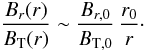 (48)In particular, at
r = r1 = 1
AU ~ 200 R⊙, it is
|Br(r1)| ≃ BT(r1).
Then, from Eq. (48) it follows that
B is quasi-radial at
r = r0:
(48)In particular, at
r = r1 = 1
AU ~ 200 R⊙, it is
|Br(r1)| ≃ BT(r1).
Then, from Eq. (48) it follows that
B is quasi-radial at
r = r0: 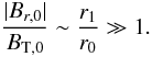 (49)The magnetic field
intensity B decreases between r0 and
r1 by a factor
(49)The magnetic field
intensity B decreases between r0 and
r1 by a factor 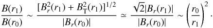 (50)The wavevector
radial component kr remains constant during
expansion, while the transverse components kTi
decrease proportional to
r0/r:
(50)The wavevector
radial component kr remains constant during
expansion, while the transverse components kTi
decrease proportional to
r0/r: 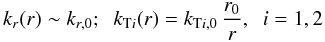 (51)where
kTi,0 = kTi(r = r0).
At r = r0 the wavevector
k associated with the discontinuity is essentially
perpendicular to B (Eq. (46)), i.e., it is quasi-transverse to the radial direction:
(51)where
kTi,0 = kTi(r = r0).
At r = r0 the wavevector
k associated with the discontinuity is essentially
perpendicular to B (Eq. (46)), i.e., it is quasi-transverse to the radial direction:
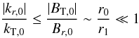 (52)where we used
Eq. (49) and
(52)where we used
Eq. (49) and
 . In
particular, the wavevector modulus is
k(r0) ≃ kT(r0).
At distance r1, using Eqs. (51) and (52) we find
. In
particular, the wavevector modulus is
k(r0) ≃ kT(r0).
At distance r1, using Eqs. (51) and (52) we find
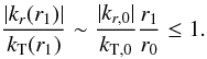 (53)This implies
 , so that we can estimate the
modulus of k at distance r1 as
k(r1) ~ kT(r1).
Then, k decreases between r0 and
r1 by a factor
, so that we can estimate the
modulus of k at distance r1 as
k(r1) ~ kT(r1).
Then, k decreases between r0 and
r1 by a factor  (54)where we used
Eq. (51). The radial evolution of the
angle θ between k and
B can now be derived: Eqs. (47) and (51) imply
(54)where we used
Eq. (51). The radial evolution of the
angle θ between k and
B can now be derived: Eqs. (47) and (51) imply
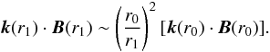 (55)Using Eqs. (50), (54), and (55) we finally obtain
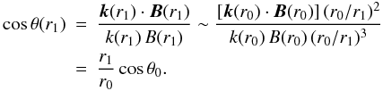 (56)Thus,
between r0 and r1 we find that
cosθ is increased by a factor
r1/r0 ≃ 200,
owing to wind expansion effects. However, since
cosθ0 ~ 10-7 (Eq. (46)), we still find that
cosθ(r1) ≪ 1. In other words, the property
that the wavevector k associated with the discontinuity is
nearly perpendicular to the ambient magnetic field is still preserved by expansion effects
at distances r ~ 1 AU.
(56)Thus,
between r0 and r1 we find that
cosθ is increased by a factor
r1/r0 ≃ 200,
owing to wind expansion effects. However, since
cosθ0 ~ 10-7 (Eq. (46)), we still find that
cosθ(r1) ≪ 1. In other words, the property
that the wavevector k associated with the discontinuity is
nearly perpendicular to the ambient magnetic field is still preserved by expansion effects
at distances r ~ 1 AU.
Concerning nonlinear effects, they have enough time to act on fluctuations during their journey from the corona to 1 AU. Thus, we expect that the originally planar discontinuity is curved and distorted, while it is advected in the surrounding turbulent medium. However, from a general point of view, nonlinear effects tend to move energy to small scales, thus we can expect that the existence of the discontinuity itself is somehow preserved by nonlinearities. Moreover, the nonlinear cascade preferentially takes place in the transverse direction to B0. Thus, nonlinear effects should “help” the discontinuity to remain quasi-perpendicular, at least locally.
The above considerations suggest that the character of the discontinuities predicted by our model should be essentially preserved in the solar wind. Of course, a more detailed analysis is well beyond the purpose of the paper. In conclusion, the mechanism analysed in the present model could explain the formation of at least a fraction of the most common kind of discontinuities detected in the solar wind.
Acknowledgments
The author is grateful to A. Greco and to F. Pucci for many stimulating discussions on the subject of the paper.
References
- Banerjee, D., Gupta, G. R., & Teriaca, L. 2011, Space Sci. Rev., in press [Google Scholar]
- Belcher, J. W., & Davis, L. 1971, J. Geophys. Res., 76, 3534 [NASA ADS] [CrossRef] [Google Scholar]
- Bruno, R., Carbone, V., Veltri, P., Pietropaolo, E., & Bavassano, B. 2001, Planet. Space Sci., 49, 1201 [Google Scholar]
- Borowsky, J. E. 2008, J. Geophys. Res., 113, 8110 [CrossRef] [Google Scholar]
- Burlaga, L. F. 1969, Sol. Phys., 7, 54 [NASA ADS] [CrossRef] [Google Scholar]
- Burlaga, L. F., & Ness, N. F. 1969, Sol. Phys., 9, 467 [NASA ADS] [CrossRef] [Google Scholar]
- Califano, F., Chiuderi, C., & Einaudi, G. 1990, ApJ, 365,757 [NASA ADS] [CrossRef] [Google Scholar]
- Califano, F., Chiuderi, C., & Einaudi, G. 1992, ApJ, 390, 560 [NASA ADS] [CrossRef] [Google Scholar]
- Carbone, V., & Veltri, P. 1990, Geophys. Astrophys. Fluid Dyn., 52, 153 [NASA ADS] [CrossRef] [Google Scholar]
- Cohen, R. H., & Kulsrud, R. M. 1974, Phys. Fluids, 17, 2215 [NASA ADS] [CrossRef] [Google Scholar]
- Davila, J. M. 1987, ApJ, 317, 514 [NASA ADS] [CrossRef] [Google Scholar]
- Greco, A., Chuychai, P., Matthaeus, W. H., Servidio, S., & Dmitruk, P. 2008, Geophys. Res. Lett., 35, L19111 [NASA ADS] [CrossRef] [Google Scholar]
- Greco, A., Matthaeus, W. H., Servidio, S., Chuychai, P., & Dmitruk, P. 2009, ApJ, 621, L111 [NASA ADS] [CrossRef] [Google Scholar]
- Heyvaerts, J., & Priest, E. R. 1983, A&A, 117, 220 [NASA ADS] [Google Scholar]
- Hollweg, J. 1987, ApJ, 312, 880 [NASA ADS] [CrossRef] [Google Scholar]
- Horbury, T., Burgess, D., Fränz, M. J., & Owen, C. J. 2001, Geophys. Res. Lett., 28, 677 [NASA ADS] [CrossRef] [Google Scholar]
- Kappraff, J. M., & Tataronis, J. A. 1977, J. Plasma Phys., 18, 209 [NASA ADS] [CrossRef] [Google Scholar]
- Knetter, T., Neubauer, F. M., Horbury, T., & Balogh, A. 2003, Adv. Space Res., 32, 543 [NASA ADS] [CrossRef] [Google Scholar]
- Knetter, T., Neubauer, F. M., Horbury, T., & Balogh, A. 2004, J. Geophys. Res., 101, A06102 [NASA ADS] [CrossRef] [Google Scholar]
- Landi, S., Velli, M., & Einaudi, G. 2005, ApJ, 624, 392 [NASA ADS] [CrossRef] [Google Scholar]
- Lee, E. M., & Roberts, B. 1986, ApJ, 301, 430 [NASA ADS] [CrossRef] [Google Scholar]
- Lee, L. C., Lin, Y., & Choe, G. S. 1996, Sol. Phys., 163, 335 [NASA ADS] [Google Scholar]
- McLaughlin, J. A., Hood, A. W., & De Moortel, I. 2010, Space Sci. Rev., doi:10.1007/s11214-010-9654-y [Google Scholar]
- Malara, F., & Elaoufir, J. 1991, J. Geophys. Res., 96, 7641 [NASA ADS] [CrossRef] [Google Scholar]
- Malara, F., Veltri, P., Chiuderi, C., & Einaudi, G. 1992, ApJ, 396, 297 [NASA ADS] [CrossRef] [Google Scholar]
- Malara, F., Primavera, L., & Veltri, P. 1996, ApJ, 459, 347 [NASA ADS] [CrossRef] [Google Scholar]
- Malara, F., Petkaki, P., & Veltri, P. 2000, ApJ, 533, 523 [NASA ADS] [CrossRef] [Google Scholar]
- Malara, F., De Franceschis, M. F., & Veltri, P. 2003, A&A, 412, 529 [NASA ADS] [CrossRef] [EDP Sciences] [Google Scholar]
- Malara, F., De Franceschis, M. F., & Veltri, P. 2005, A&A, 443, 1033 [NASA ADS] [CrossRef] [EDP Sciences] [Google Scholar]
- Malara, F., Veltri, P., & De Franceschis, M. F. 2007, A&A, 467, 1275 [NASA ADS] [CrossRef] [EDP Sciences] [Google Scholar]
- Mariani, F., Bavassano, B., & Villante, U. 1983, Sol. Phys., 83, 349 [NASA ADS] [CrossRef] [Google Scholar]
- Martin, R. N., Betcher, J. W., & Lazarus, A. J. 1991, J. Geophys. Res., 78, 3653 [NASA ADS] [CrossRef] [Google Scholar]
- Matthaeus, W. H., Ghosh, S., Oughton, S., & Roberts, D. A. 1996, J. Geophys. Res., 101, 7619 [NASA ADS] [CrossRef] [Google Scholar]
- Mok, Y., & Einaudi, G. 1985, J. Plasma Phys., 33, 199 [NASA ADS] [CrossRef] [Google Scholar]
- Müller, W.-C., & Grappin, R. 2005, Phys. Rev. Lett., 95, 114502 [NASA ADS] [CrossRef] [Google Scholar]
- Nakariakov, V. M., Roberts, B., & Murawski, K. 1997, Sol. Phys., 175, 93 [NASA ADS] [CrossRef] [Google Scholar]
- Nakariakov, V. M., Roberts, B., & Murawski, K. 1998, A&A, 332, 795 [NASA ADS] [Google Scholar]
- Neugebauer, M. 1989, Geophys. Res. Lett., 16, 1261 [NASA ADS] [CrossRef] [Google Scholar]
- Neugebauer, M. 2006, J. Geophys. Res., 111, A04103 [NASA ADS] [CrossRef] [Google Scholar]
- Owens, M. J., Wicks, R. T., & Horbury, T. S. 2011, Sol. Phys., 269, 411 [NASA ADS] [CrossRef] [Google Scholar]
- Petkaki, P., Malara, F., & Veltri, P. 1998, ApJ, 500, 483 [NASA ADS] [CrossRef] [Google Scholar]
- Pommois, P., Zimbardo, G., & Veltri, P. 1998, Phys. Plasmas, 5, 1288 [NASA ADS] [CrossRef] [Google Scholar]
- Ruderman, M. S., Nakariakov, V. M., & Roberts, B. 1998, A&A, 338, 1118 [NASA ADS] [Google Scholar]
- Shebalin, J. V., Matthaeus, W. H., & Montgomery, D. 1983, J. Plasma Phys., 78, 2088 [Google Scholar]
- Similon, P. L., & Sudan, R. N. 1989, ApJ, 336, 442 [NASA ADS] [CrossRef] [Google Scholar]
- Smith, E. J. 1973, J. Geophys. Res., 78, 2088 [NASA ADS] [CrossRef] [Google Scholar]
- Soding, A., Neubauer, F. M., Tsurutani, B., Ness, N. F., & Lepping, R. P. 2001, Ann. Geophys., 19, 681 [NASA ADS] [CrossRef] [Google Scholar]
- Steinolfson, R. S. 1985, ApJ, 295, 213 [NASA ADS] [CrossRef] [Google Scholar]
- Tomczyk, S., & McIntosh, S. W. 2009, ApJ, 697, 1384 [NASA ADS] [CrossRef] [Google Scholar]
- Tsurutani, B. T., & Smith, E. J. 1979, J. Geophys. Res., 84, 2773 [NASA ADS] [CrossRef] [Google Scholar]
- Vasquez, B. J. 2005, in Proceedings of the Conference Solar Wind 11 – SOHO 16, Simulation study of waves supported by tangential discontinuities, eds. B. Fleck, & T. H. Zurbuchen, ESA Publ., SP-592, 649 [Google Scholar]
- Vasquez, B. J., & Hollweg, J. V. 1996, J. Geophys. Res., 101, 13527 [NASA ADS] [CrossRef] [Google Scholar]
- Vasquez, B. J., & Hollweg, J. V. 1998, J. Geophys. Res., 103, 335 [NASA ADS] [CrossRef] [Google Scholar]
- Vasquez, B. J., Abramenko, V. I., Haggerty, D. K., & Smith, C. W. 2007, J. Geophys. Res., 112, A11102 [NASA ADS] [CrossRef] [Google Scholar]
- Verdini, A., Velli, M., & Buchlin, E. 2009, ApJ, 700, L39 [NASA ADS] [CrossRef] [Google Scholar]
- Zhang, J., Ma, J., & Wang, H. 2006, ApJ, 649, 464 [NASA ADS] [CrossRef] [Google Scholar]
- Zimbardo, G., Veltri, P., & Malara, F. 1984, J. Plasma Phys., 32, 141 [NASA ADS] [CrossRef] [Google Scholar]
Appendix A: Energy spectrum
In this appendix we derive Eqs. (35) and (36) for the energy spectrum in the homogeneous region. In this derivation we use some results by Malara et al. (2007), which we briefly illustrate in the following.
Let us consider two points in the Alfvénic perturbation x(t) and x′(t) = x(t) + δx(t) that propagate along two nearby rays, where δx(t) is the infinitesimal vector difference. During propagation both k and δx are modified, but the quantity k δx|| remains constant, δx|| being the component of δx parallel to k (Malara et al. 2007). This fact has two implications:
-
a)
Considering a vector difference δx that is initially perpendicular to k (δx|| = 0), it will remain perpendicular to k all along the ray. At any given time t, a wavefront is any surface where the phase function F(x,t) is constant. Property a) can be expressed in the following form. If initially δx lies on a given wavefront, it will remain on the same wavefront during propagation.
-
b)
If initially δx|| ≠ 0, then the following ratio is constant during propagation:
 (A.1)where
λ = 2π/k is the local
wavelength.
(A.1)where
λ = 2π/k is the local
wavelength.
Using three noncoplanar vector differences δxA, δxB, and δxC, an infinitesimal volume δV = |δxA·(δxB × δxC)| within the perturbation can be defined. The portion of perturbation contained in δV is indicated as a “packet”. Packets propagate along rays. If ρ(0) is uniform, the volume δV remains constant during propagation (Malara et al. 2007). The energy associated with a packet is δE = ⟨ e ⟩ δV and it remains constant during propagation, as long as dissipation is neglected, as in the present case.
Let us consider the perturbation at the base z = 0, in the area where
open magnetic lines have their origin; the corresponding surface has been indicated by
Sopen. This perturbation is divided into
Nopen small equal packets, each one having the same volume
δV and carrying the same energy δE. We choose such
packets as small cubes with the side
δxA
parallel to the initial wavevector k0, while the
two other sides,
δxB and
δxC, are
perpendicular to k0, i.e., they lie on a
wavefront. Then, each packet is contained between two parallel wavefronts. The above
property a) implies that the packet, while propagating, remains in between two wavefronts
for all subsequent times. In the limit of large Nopen the
linear size of such packets at z = 0 is  (A.2)and the energy
carried by the packet is
(A.2)and the energy
carried by the packet is 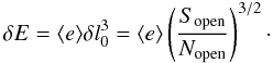 (A.3)These packets
propagate following open magnetic lines, and eventually reach the region of homogenous
magnetic field. Inside the homogeneous region we select a subdomain
Dh in the form of a parallelepiped: the base of
Dh is equal to the base S of the whole
domain D, while the height Lh of
Dh is arbitrary. In a stationary situation, at any time, the
subdomain Dh is filled by packets coming from the base
z = 0. Packets that were initially cubic have been deformed crossing
the underlying inhomogeneous region, and they became parallelepipeds with nonorthogonal
sides. However, packets do not deform any more inside Dh, but
they simply propagate in the z direction at a constant speed. Then, at
any given time, for given values of x and y moving along
z inside Dh, we find a sequence of packets
all having the same geometrical shape and the same value of the wavevector. We identify
each of these “columns” of equal packets by the index α, and
kα is the value of the
wavevector of all the packets in the α-th column. In the column each
packet is separated from the subsequent one by a wavefront. The distance between two of
these wavefronts, measured along the z direction, is
(A.3)These packets
propagate following open magnetic lines, and eventually reach the region of homogenous
magnetic field. Inside the homogeneous region we select a subdomain
Dh in the form of a parallelepiped: the base of
Dh is equal to the base S of the whole
domain D, while the height Lh of
Dh is arbitrary. In a stationary situation, at any time, the
subdomain Dh is filled by packets coming from the base
z = 0. Packets that were initially cubic have been deformed crossing
the underlying inhomogeneous region, and they became parallelepipeds with nonorthogonal
sides. However, packets do not deform any more inside Dh, but
they simply propagate in the z direction at a constant speed. Then, at
any given time, for given values of x and y moving along
z inside Dh, we find a sequence of packets
all having the same geometrical shape and the same value of the wavevector. We identify
each of these “columns” of equal packets by the index α, and
kα is the value of the
wavevector of all the packets in the α-th column. In the column each
packet is separated from the subsequent one by a wavefront. The distance between two of
these wavefronts, measured along the z direction, is  (A.4)where
θα is the angle between
kα and the
z direction. Equations (A.1) and (A.2) imply that
(A.4)where
θα is the angle between
kα and the
z direction. Equations (A.1) and (A.2) imply that
 (A.5)with
λα = 2π/kα
and
λ0 = 2π/k0.
Using Eq. (A.5) and the relation
|kz,α| = kαcosθα,
Eq. (A.4) implies
(A.5)with
λα = 2π/kα
and
λ0 = 2π/k0.
Using Eq. (A.5) and the relation
|kz,α| = kαcosθα,
Eq. (A.4) implies  (A.6)The number of
packets forming the αth column within the subdomain
Dh is
Nα = Lh/δlz,α.
Therefore, using Eqs. (A.3) and (A.6), the αth column
contributes with the energy
(A.6)The number of
packets forming the αth column within the subdomain
Dh is
Nα = Lh/δlz,α.
Therefore, using Eqs. (A.3) and (A.6), the αth column
contributes with the energy 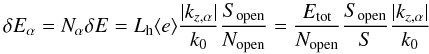 (A.7)where
Etot = ⟨ e ⟩ SLh
is the energy contained in the whole domain Dh.
(A.7)where
Etot = ⟨ e ⟩ SLh
is the energy contained in the whole domain Dh.
We now divide the k axis into a sequence of adjacent bins
I(k); each bin has amplitude Δk and
is centred on a value k. We select all the packets whose wavevector
kα falls into the bin
I(k): the total energy of these packets is
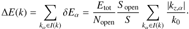 (A.8)The energy
spectrum per unit volume in the homogeneous region is defined as
ϵ(k) = ΔE(k)/(SLh Δk).
Using Eq. (A.8) we find
(A.8)The energy
spectrum per unit volume in the homogeneous region is defined as
ϵ(k) = ΔE(k)/(SLh Δk).
Using Eq. (A.8) we find 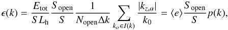 (A.9)where
 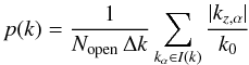 (A.10)the
last two equations are Eqs. (35)
and (36), respectively.
(A.10)the
last two equations are Eqs. (35)
and (36), respectively.
All Figures
|
Fig. 1 Vertical component |
| In the text | |
|
Fig. 2 Magnetic lines of the equilibrium magnetic field B(0), for μ = 4/3. |
| In the text | |
|
Fig. 3 Distribution p(k) as a function of the normalized wavevector k/k0, calculated for different values of the parameters μ and nmax of the equilibrium magnetic field B(0). The quantity p(k) is proportional to the fluctuation spectrum per unit volume ϵ(k) in the homogeneous region. A power law with slope −α = −2.3 is also shown for comparison. |
| In the text | |
|
Fig. 4 Scatter plot with the values k||/k0 and k⊥/k0 displayed on the horizontal and vertical axes, respectively. These values are calculated for N = 10 000 rays at z = zh, in the case μ = 1.33, nmax = 10. |
| In the text | |
|
Fig. 5 Unit vectors K (arrows) giving the direction of wavevectors k of large-scale structures, at z = zh, projected on the horizontal xy plane. The starting points of each unit vector (large square dots) are the (x,y) positions of the corresponding rays at z = zh. The dotted area represents the area at the base z = 0 where Bz ≥ 0. The segment AB is also plotted. |
| In the text | |
|
Fig. 6 Segment AB (straight full line), the two portions
|
| In the text | |
|
Fig. 7 Wavevector k (full line) and the phase function F (dashed line) as functions of the coordinate ξ along the segment AB. |
| In the text | |
|
Fig. 8 Wavevector component k·u as a function of |ξ − ξC| for ξ < ξC (crosses) and for ξ > ξC (circles). A function proportional to |ξ − ξC|-0.85 (full line) is plotted for comparison. |
| In the text | |
Current usage metrics show cumulative count of Article Views (full-text article views including HTML views, PDF and ePub downloads, according to the available data) and Abstracts Views on Vision4Press platform.
Data correspond to usage on the plateform after 2015. The current usage metrics is available 48-96 hours after online publication and is updated daily on week days.
Initial download of the metrics may take a while.