| Issue |
A&A
Volume 548, December 2012
|
|
|---|---|---|
| Article Number | A124 | |
| Number of page(s) | 8 | |
| Section | Interstellar and circumstellar matter | |
| DOI | https://doi.org/10.1051/0004-6361/201219871 | |
| Published online | 04 December 2012 | |
Discovery of an outflow of the very low-mass star ISO 143⋆
1 Universität Heidelberg, Zentrum für Astronomie, Institut für Theoretische Astrophysik Albert-Ueberle-Str. 2, 69120 Heidelberg, Germany
e-mail: This email address is being protected from spambots. You need JavaScript enabled to view it.
2 Max-Planck Institut für Astronomie, Königstuhl 17, 69117 Heidelberg, Germany
Received: 22 June 2012
Accepted: 27 September 2012
Abstract
We discover that the very young very low-mass star ISO 143 (M5) is driving an outflow based on spectro-astrometry of forbidden [S II] emission lines at 6716 Å and 6731 Å observed in UVES/VLT spectra. This adds another object to the handful of brown dwarfs and very low-mass stars (M5-M8) for which an outflow has been confirmed and which show that the T Tauri phase continues at very low masses. We find the outflow of ISO 143 to be intrinsically asymmetric and the accretion disk to not obscure the outflow, as only the red outflow component is visible in the [S II] lines. ISO 143 is only the third T Tauri object showing a stronger red outflow component in spectro-astrometry, after RW Aur (G5) and ISO 217 (M6.25). We show here that, including ISO 143, two out of seven outflows confirmed in the very low-mass regime (M5-M8) are intrinsically asymmetric. We measure a spatial extension of the outflow in [S II] of up to 200–300 mas (about 30–50 AU) and velocities of up to 50–70 km s-1. We furthermore detect line emission of ISO 143 in Ca II (8498 Å), O I (8446 Å), He I (7065 Å), and weakly in [Fe II] (7155 Å). Based on a line profile analysis and decomposition we demonstrate that (i) the Ca II emission can be attributed to chromospheric activity, a variable wind, and the magnetospheric infall zone, (ii) the O I emission mainly to accretion-related processes but also a wind, and (iii) the He I emission to chromospheric or coronal activity. We estimate a mass outflow rate of ISO 143 of ~10-10 M⊙ yr-1 and a mass accretion rate in the range of ~10-8 to ~10-9 M⊙ yr-1. These values are consistent with those of other brown dwarfs and very low-mass stars. The derived Ṁout/Ṁacc ratio of 1–20% does not support previous findings of this number being very large (>40%) for very low-mass objects.
Key words: stars: low-mass / stars: pre-main sequence / circumstellar matter / stars: individual: ISO 217 / stars: winds, outflows / techniques: high angular resolution
Based on observations obtained at the Very Large Telescope of the European Southern Observatory at Paranal, Chile in program 080.C- 0904(A) 082.C-0023(A+B).
© ESO, 2012
1. Introduction
While many details of the origin of brown dwarfs are still unknown, it was established in the last few years that during their early evolution brown dwarfs resemble higher mass T Tauri stars in main properties. Very young brown dwarfs (a few Myr) show surface activity, such as cool spots (e.g., Joergens et al. 2003). There is evidence that brown dwarfs have disks from mid-infrared (mid-IR, e.g., Comerón et al. 2000; Jayawardhana et al. 2003; Luhman et al. 2008) and far-IR/submm excess emission (Klein et al. 2003; Scholz et al. 2006; Harvey et al. 2012a,b). Many of these disks have been found to be actively accreting (e.g., Mohanty et al. 2005; Herczeg & Hillenbrand 2008; Bacciotti et al. 2011; Rigliaco et al. 2011), and several show signs of grain growth and crystallization (e.g., Apai et al. 2005; Pascucci et al. 2009). Furthermore, very young brown dwarfs rotate on average more slowly (e.g., Joergens & Guenther 2001; Joergens et al. 2003; Caballero et al. 2004) than their older counterparts (e.g., Bailer-Jones & Mundt 2001; Mohanty & Basri 2003), which is indicative of a magnetic braking mechanism due to interaction with the disk.
Jets and outflows are known to be a by-product of accretion in the star-formation process, and they have been observed for many classical T Tauri stars (CTTS, e.g., Ray et al. 2007, for a review). It has recently been shown that brown dwarfs and very low-mass stars (VLMS) are also able to drive T Tauri-like outflows based on the detection of forbidden emission lines (FELs, e.g., Fernandez & Comerón 2001; Looper et al. 2010), spectro-astrometry of FELs (Whelan et al. 2005, 2007, 2009a,b; Bacciotti et al. 2011; Joergens et al. 2012), and direct imaging in the CO J = 2–1 transition (Phan-Bao et al. 2008). To date, outflows have been confirmed for six M5 to M8 type brown dwarfs and VLMS providing evidence that objects of a tenth of a solar mass to less than 30 MJup can launch powerful outflows: Par-Lup3-4 (M5), ρ Oph 102 (M5.51), ISO 217 (M6.25), LS-R CrA 1 (M6.5), 2M1207 (M8), and ISO-Oph 32 (M8).
Observing log of ISO 143.
We present here the discovery of an outflow of the VLMS ISO 143 (M5) based on the spectro-astrometry of [S II] lines in high-resolution UVES/VLT spectra. This adds another object to the small sample of detected outflows for brown dwarfs and VLMS. We investigate the outflow properties of ISO 143. Furthermore, we show that ISO 143 exhibits several other activity-related emission lines and localize their formation sites.
The paper is organized as follows: After a summary of the known properties of ISO 143 (Sect. 2), the acquisition and analysis of high-resolution UVES/VLT spectra is described (Sect. 3). In Sect. 4, the results of the emission line study and the spectro-astrometric detection of the outflow is presented, followed by our conclusions on ISO 143 in Sect. 5.
2. The very low-mass star ISO 143
ISO 1432 is a very low-mass star of spectral type M5 situated in the Cha I star-forming region (Luhman 2007). An estimate of its mass based on a comparison of effective temperature and luminosity (Teff = 3125 K, Lbol = 0.088 L⊙, Luhman 2007) with evolutionary models (Baraffe et al. 1998) yields a value of 0.18 M⊙. ISO 143 exhibits mid- and far-IR excess emission providing evidence of a circumstellar disk. These detections were made with the InfraRed Array Camera (IRAC) on board the Spitzer satellite (3.6, 4.5, 5.8, 8.0 μm), the Multiband Imaging Photometer for Spitzer (MIPS, 24 μm, Damjanov et al. 2007; Luhman et al. 2008), and the Photoconductor Array Camera and Spectrometer (PACS) of the Herschel mission (70, 160 μm, Harvey et al. 2012b). An IR spectrum of ISO 143 taken by the Spitzer/InfraRed Spectrograph (IRS, 5–36 μm) shows a weak 10 μm silicate feature (Manoj et al. 2011). ISO 143 was classified as a class II source based on the spectral slope between 8 μm and 24 μm (Luhman et al. 2008; Manoj et al. 2011). The disk appears to be relatively flat and to have undergone substantial dust settling (Manoj et al. 2011). Modeling of its spectral energy distribution (SED), including Herschel/PACS data at 70 μm and 160 μm (Harvey et al. 2012b; Y. Liu, priv. comm.), yields a total disk mass of 5 × 10⁻⁶ M⊙ (assuming a standard gas-to-dust ratio of 100), a disk flaring index of less than 1.1, and an inclination less than 60°, with the most likely value being 15°–25°, i.e. close to face on, although inclination values 0°–50° are almost equally likely. ISO 143 shows Hα in emission with an equivalent width of 118 Å (Luhman 2004), indicating that the disk is actively accreting.
3. High-resolution spectra and spectro-astrometry
We observed ISO 143 with the Ultraviolet and Visual Echelle Spectrograph (UVES, Dekker et al. 2000) attached to the VLT 8.2 m KUEYEN telescope in three nights in 2008 and 2009 in the red optical wavelength regime at a spectral resolution λ/Δλ of 40 000. The spatial sampling was 0.182′′/pixel. An observing log is given in Table 1.
We used UVES spectra that were reduced, wavelength-, and flux-calibrated by means of the ESO UVES pipeline in order to study activity related emission lines (Ca II, O I, He I, [S II], [Fe II]) regarding their line profile shapes (Sect. 4.1). Furthermore, a spectro-astrometric analysis of the detected forbidden line emission in [S II] was performed based on a custom-made reduction and wavelength calibration procedure. After completing a standard CCD reduction of the raw data (bias and flatfield correction and cosmic-ray elimination), a row-by-row wavelength calibration of the two-dimensional spectra of individual echelle orders was done using the longslit package (fitcoords/transform) of IRAF. Finally, the sky was subtracted. We measured the spectro-astrometric signature in the resulting two-dimensional spectra by Gaussian fitting the spatial profile at each wavelength of both the FELs and the adjacent continuum, following, e.g., Hirth et al. (1994a). The spatial offset in the FEL was then computed relative to the continuum. To increase the signal-to-noise ratio (S/N), which is the limiting factor in applying spectro-astrometry to faint objects, the data were binned in the wavelength direction. To rule out spectro-astrometric artifacts, which can be caused, for example, by an asymmetric PSF (Brannigan et al. 2006), we applied spectro-astrometry to a photospheric absorption line (K I λ7699) and demonstrated that the spectro-astrometric offset in this line does not exceed 50 mas (apart from one outlier, see Fig. 1, top row). Further details on the spectro-astrometric analysis can be found in Joergens et al. (2012).
Slit position angle. The UVES observations of ISO 143 were obtained within the framework of a high-resolution spectroscopic study of young brown dwarfs and VLMS that is optimized for radial velocity work (e.g., Joergens 2008a). Therefore, the slit orientation was kept aligned with the direction of the atmospheric dispersion, and, as a consequence, changed relative to the sky during the observations. Each 2 × 1700 s exposure samples a range of on-sky slit position angles (PAs) of about ±8°, as given in Table 1. Despite the slit PA varying during the exposure, the data nonetheless allowed the detection of outflows, as shown by our confirmation of the bipolar outflow of ISO 217 (Joergens et al. 2012) and by the spectro-astrometry of ISO 143 presented here. The spectra of ISO 143 were taken at mean slit PAs of 3°, 10°, and 40°, which enabled us to investigate the observed outflow extension as a function of the slit PA (see Sect. 4.2).
Stellar rest velocity. A value of V0 = 16.9 km s-1 was adopted for the stellar rest velocity of ISO 143, which is the mean value of the radial velocities measured for ISO 143 based on a cross correlation of many photospheric lines in the same spectra (Joergens, in prep.; cf. Table 1). All velocities in the following are given relative to this value of V0.
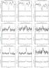 |
Fig. 1 Spectro-astrometric analysis of spectral lines of ISO 143 for three different observing times and slit PAs. Top row: photospheric line K I λ7699 as a test for artifacts, middle row: FEL of [S II] λ6716, bottom row: FEL of [S II] λ6731. For each case, we display the line profiles in the top panels, which are the average of 8 pixel rows in the spatial direction centered on the continuum after continuum subtraction, and the spectro-astrometric plots in the bottom panels, which show the spatial offset vs. radial velocity of the continuum (black asterisks) and of the continuum subtracted spectral line (red squares). Velocities are given relative to the stellar rest velocity V0 of ISO 143. |
Observed emission lines of ISO 143.
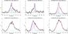 |
Fig. 2 Emission lines of Ca II λ8498 (top row) and O I λ8446 (bottom row) in UVES spectra of ISO 143 at different observing times in Mar. 2008, Jan. 2009, and Feb. 2009 in the order of increasing slit PA after continuum subtraction. The flux is given in arbitrary units. Gaussian fitting shows that the Ca II line can be decomposed into three components: (i) a narrow one centered close to zero velocity (probably chromospheric, green dotted line), (ii) a broader blue-shifted one (possibly produced in a wind, blue dotted line), and (iii) a very broad red-shifted one (possibly produced in magnetospheric infall, red dotted line). The pink dashed line is the sum of the Gaussian functions. The O I line can be fitted by a single red-shifted component in the two spectra from 2009 and by a blue- and a red-shifted component in the spectrum from 2008 (the pink dashed line denotes here the sum of the two Gaussian functions). |
4. Results
4.1. Observed emission lines
The observations of ISO 143 at high spectral resolution with UVES reveal line emission in Ca II, O I, He I, [S II], and [Fe II], which are signatures of chromospheric activity, ongoing accretion, winds, and/or outflowing material. We studied their line profile shapes, measured their equivalent widths (EWs) and full-width-at-half-maximum values (FWHMs) in order to localize their formation sites in the system. For this purpose, we used the UVES spectra (Table 1) after reduction, wavelength-, and flux-calibration by the ESO UVES pipeline. Furthermore, a polynomial fit to the continuum emission adjacent to each line was subtracted from the emission line regions. Several emission line profiles of ISO 143 display complex shapes that obviously consist of more than one emission component. We decomposed these line profiles into its constituent components using the IRAF task ngaussfit. We fitted up to three Gaussian functions to the profiles leaving the peak flux, velocity at the peak, and FWHM for each component as free parameters. We furthermore measured EWs for each line component. Table 2 lists the observed emission lines, the determined peak radial velocities V, FWHMs, and EWs for each individual component. Details on the individual emission lines are presented in the following.
Ca II IR emission. ISO 143 exhibits a broad, asymmetric, and variable Ca II IR emission line at 8498 Å, which clearly consists of more than one component. Figure 2 displays this line at three different epochs in 2008 and 2009 in the top panels. We note that the two other lines of this IR triplet are not covered by the observations because of a gap in wavelength between the CCD chips of the two-armed spectrograph. A decomposition of the Ca II line profile into its constituent components demonstrates that it can be fitted by three Gaussian functions (Fig. 2): (i) a narrow emission component, which is centered close to zero velocity; (ii) a broader blue-shifted component; and (iii) a very broad red-shifted component. The narrow emission component (peak at velocities between −1 km s-1 and 7 km s-1; FWHM of 9–21 km s-1, EW of 0.1–0.7 Å) is attributed to chromospheric activity giving its narrow profile centered close to the stars velocity. The variability of a few km s-1 seen in this line component (Table 2) but not in the velocity of the star (Table 1) could be explained by rotational modulation caused by inhomogenously distributed activity regions in the chromosphere, such as plages (e.g., Huerta et al. 2008; Joergens 2008b; Prato et al. 2008, for T Tauri related activity causing velocity variability of a few km s-1; e.g., Berdyugina 2005, for Ca II emission produced in the chromosphere/chromospheric plages). The broader blue-shifted component in Ca II (peak at velocities between −1 km s-1 and −36 km s-1; FWHM of 41–60 km s-1; EW of 0.6–0.9 Å) is suggested to be the signature of a wind that is expanding at a variable velocity. The very broad red-shifted emission component (peak at 26–63 km s-1; FWHM of 94–165 km s-1; EW of 0.6–4.1 Å), which is significantly variable in both the peak velocity (ΔV = 37 km s-1) and strength (ΔEW = 3.5 Å), is likely formed in the magnetospheric infall zone of the system (cf. Muzerolle et al. 1998, for Ca II emission from infalling material in CTTS). The sum of the three individual Gaussians (Fig. 2, top panels, pink dashed line), is the overall fit to the Ca II profile.
O I emission. ISO 143 has strong, broad, and variable emission in the O I line at 8446 Å (Fig. 2, bottom panels). This emission is centered on red-shifted velocities in the two spectra from 2009 and on blue-shifted velocities in the spectrum from 2008. We show that the line can be fitted by a single red-shifted Gaussian function for the two spectra in 2009 and that it can be decomposed into a blue- and a red-shifted component in the spectrum from 2008. The profile of the red component of this O I line has a very broad velocity distribution (FWHM of 106–121 km s-1) and a peak at velocities that are moderately red-shifted (9–19 km s-1) but not as strong as seen in the red component of Ca II. The red component of O I is significantly variable in both the peak velocity (ΔV = 10 km s-1) and strength (ΔEW = 3.4 Å). We attribute the emission in the red component mainly to disk accretion and, to a lesser extent, also to infalling material. The blue component that appears in this line in 2008 has approximately the same velocity (−42 km s-1) as the blue component in the Ca II line at the same epoch (−36 km s-1) suggesting a common origin in a variable wind.
He I emission. We detect a prominent He I emission line at 7065 Å (Figs. 3, 4). The relatively narrow-band profile (FWHM of 26–35 km s-1) of this line being centered on V = 0 and displaying little variability in its strength (ΔEW ≤ 0.1 Å), and the high temperature and density required to excite this transition indicates an origin in the chromosphere or the transition zone between the chromosphere and the corona (cf. e.g. Sicilia-Aguilar et al. 2012). We note that a second weaker blended He I line at 7065.7 Å emerges in the red wing of this He I line at 7065.2 Å (Fig. 3).
Forbidden [S II] emission. ISO 143 shows strong emission in forbidden lines of sulfur [S II] at 6716 Å and 6731 Å (Fig. 1) with a velocity at the line peak of 41–50 km s-1, a FWHM of 27–33 km s-1, and an EW of 0.2 Å for [S II]λ6716 and of 0.4–0.5 Å for [S II]λ6731 (Table 2). The [S II] line profiles appear to vary little both in their strength (ΔEW ≤ 0.1 Å) and peak velocity (ΔV ≲ 1 km s-1, with the exception of the [S II]λ6716 profile on Feb. 2009; however, here the location of the peak was hampered by a low S/N). Spectro-astrometry of these lines (Sect. 4.2) reveals that they are formed in an outflow at a distance from the central source of up to 30–50 AU. For both [S II] lines, only a red-shifted component is visible. This implies that the outflow of ISO 143 is intrinsically asymmetric and that there is either no or only little obscuration of the outflow seen in [S II] by the disk.
Forbidden [Fe II] emission. We detect weak forbidden line emission of [Fe II] at 7155 Å and tentatively at 7172 Å (Fig. 4). The peak of the [Fe II] λ7155 line seems to be around zero or low blue-shifted velocities; however, the poor S/N of this line hampers further quantitative analysis. If confirmed, the observation of solely blue-shifted forbidden [Fe II] emission of a very low-mass outflow system that has a stronger red outflow component in [S II] would resemble the case of the [Fe II] emission of the brown dwarf ISO 217 (Joergens et al. 2012).
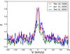 |
Fig. 3 He I λ7065 emission line in UVES spectra of ISO 143 at different observing times in 2008 and 2009 after continuum subtraction. The flux is given in arbitrary units. This He I line at 7065.2 Å is blended with another, weaker He I line at 7065.7 Å, which shows up in the red line wing at a velocity of about +30 km s-1. |
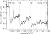 |
Fig. 4 [Fe II] λλ7155,7172 emission lines in a mean UVES spectrum of ISO 143. Also visible in this portion of the spectrum are TiO absorption bands with band-heads at 7053 Å, 7087 Å, and 7124 Å, and the He I λ7065 emission line. |
4.2. Results of spectro-astrometry
Outflow parameters from forbidden [S II] lines and mass accretion rate from the OI 8446 line.
We have clearly discovered the spectro-astrometric signature of an outflow in both [S II] lines at all three epochs in our UVES spectra of ISO 143. Figure 1 shows in the middle and bottom rows the line profiles of both the [S II] λλ6716, 6731 lines and their measured spatial offsets as a function of the velocity. The spatial offsets are displayed for both the adjacent continuum and the continuum subtracted FEL. The plotted errors in the spectro-astrometric plots are based on 1σ errors in the Gaussian fit parameters. Table 3 lists the maximum spatial offsets and corresponding velocities of both [S II] lines in the order of increasing slit PA. Offset errors in Table 3 are based on the standard deviation in the continuum points. For an overview and to constrain the outflow PA (see below), we plot the maximum spatial offsets as a function of the slit PA in Fig. 5.
Our spectro-astrometric analysis of the detected FELs of [S II] demonstrated that they originate from spatially offset positions of the continuum source by up to 200–300 mas (about 30–50 AU at the distance of Cha I) at a velocity of up to 50–70 km s-1. We found the [S II] λ6716 emission to be spatially more extended than the [S II] λ6731 emission (Table 3, Fig. 5), which is consistent with the [S II] λ6716 line tracing lower densities than the [S II] λ6731 line.
The spectra were taken at mean slit PAs of 3° ± 8°, 10° ± 8°, and 42° ± 8° (cf. Sect. 3). As illustrated in Fig. 5, we see a tendency for the estimated outflow extension to increase with increasing slit PA. The data thus hint that by varying the slit PA from 3° to 42°, one approaches the actual outflow PA. Follow-up observations, ideally spectra taken at two orthogonal slit PAs, are required to further constrain the outflow PA of ISO 143, in particular since the S/N is moderate for the spectra at 42°.
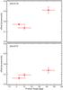 |
Fig. 5 Spatial offsets of FEL of ISO 143 as function of slit PA for [S II] λ6716 (top panel) and [S II] λ6731 (bottom panel). |
4.3. Electron density and mass outflow rate
The line intensity ratio [S II]λ6731/[S II]λ6716 can be used to derive the gas electron density ne in the line-emitting region because these two lines have nearly the same excitation energy and, therefore, their relative excitation rates only depend on the ratio of collisional strengths, i.e. on the density (Osterbrock & Ferland 2006, p. 121 ff; Bacciotti et al. 1995). We measured an [S II] line ratio for ISO 143 of 2.0 in spectra from Jan. 2009 (slit PA = 3°) and Feb. 2009 (42°, cf. Table 2) indicating an electron density ne of about 5600 cm-3. For the epoch Mar. 2008 (10°), the estimated [S II] line ratio indicates an ne value above the line critical density nc, thus only a lower limit ne > nc ~ 2 × 104 cm-3 can be derived in this case.
We proceeded to estimate the mass loss rate of ISO 143 following Hartigan et al. (1995; cf. also Comerón et al. 2003). For this purpose we derived the line luminosity of [S II]λ6731 from its measured EW (Table 2) and the dereddened R0 magnitude:  (1)We used a distance d of 162.5 pc (Luhman 2007), an R-band magnitude of 18.02 mag, which is obtained in the WFI R-band filter (López-Martí et al. 2004), and an extinction of AR(WFI) = 2.97 mag. The latter was converted from AJ = 1.13 (Luhman 2007) by interpolating the reddening law of Mathis (1990) for RV = 5.0 (Luhman 2004). The line luminosity we estimated for [S II]λ6731 in ISO 143 is 7–9 × 10⁻⁷ L⊙ (Table 3).
The mass loss rate was estimated from the line luminosity L6731 for ne < nc by the following equation (Comerón et al. 2003): 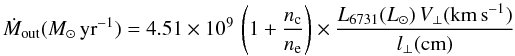 (2)where nc is the critical density and V⊥ and l⊥ are the estimated tangential flow speed and scale length of the emission. In the case of the [SII]λ6731 line that is within the high density limit (Mar. 2008, 10°), the mass loss rate does not depend upon the electron density (Hartigan et al. 1995) and Eq. (2) becomes
 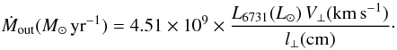 (3)For the scale length of the emitting region l⊥, we adopted the size of the aperture (cf. e.g. Hartigan et al. 1995), i.e. the UVES slit width of the observations of 1′′. For the outflow tangential velocity V⊥, we exploited the kinematic properties determined from spectro-astrometry of the [SII]λ6731 line (Table 3), which indicate a radial velocity Vr of the outflow of ISO 143 of around 50 km s-1. Although the outflow inclination is unknown in principle, we can roughly estimate the tangential velocity V⊥ from the observed Vr by assuming that the outflow direction is perpendicular to the plane of the accretion disk and using the disk inclination value derived from the SED fitting (Harvey et al. 2012b; Liu, priv. comm.). The disk inclination is, unfortunately, not very well constrained, because of the degeneracy of the SED model; the best-fit value is close to face-on (15°–25°), but disk inclination values 0°–50° are almost equally likely (cf. Sect. 2). The visibility of the red outflow component indicates an at least not completely face-on viewing angle of the disk, and we therefore adopt, somewhat arbitrarily, an outflow inclination angle of 45° for calculating the mass outflow rate, i.e. Vr = V⊥.
The estimated outflow rate for ISO 143 (0.8–3 × 10⁻¹⁰ M⊙ yr-1, Table 3) is consistent with previously determined mass loss rates of brown dwarfs and VLMS (Whelan et al. 2009a; Bacciotti et al. 2011). We note that assuming a larger outflow inclination angle, say of 65° (corresponding to a disk inclination of 25°), would result in outflow rates that are a factor of two lower than the given values. We find the same outflow rate for the observations at a slit PA of 3° and 42° indicating no significant change as a function of slit PA from these data. While we derive a smaller outflow rate for observations at 10°, this deviation in the outflow rate by a factor of about four can be traced back to a small difference in the EW value of 0.1 Å and is, therefore, not taken as sound proof of a variable mass loss rate. Interestingly, a lower mass loss rate in this epoch would correlate with a decreased mass accretion rate in this epoch (see Sect. 4.4).
4.4. Mass accretion rate
The mass accretion rate of ISO 143 was derived from the accretion luminosity, 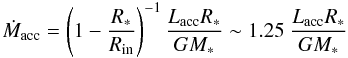 (4)(Gullbring et al. 1998), by the use of the OI λ8446 emission line as an indirect accretion tracer. We can assume that this line is predominantly produced by accretion, possibly except for the blue component we find in the profile of Mar. 2008 (cf. Sect. 4.1). We determined the line luminosity of OI λ8446 (for the spectrum of Mar. 2008 only the line luminosity of the red component) by applying Eq. (1) and using the dereddened i-band magnitude. We adopted an i-band magnitude of 15.51 mag (Luhman 2004), which was obtained in the DENIS i-band filter, and an extinction of Ai(DENIS) = 2.37 mag, which is again converted from AJ = 1.13 (Luhman 2007) by interpolating the extinction law of Mathis (1990). A comparison of the determined L8446 (see Table 3) with an empirical correlation of line and accretion luminosity for OI λ8446 (Herczeg & Hillenbrand 2008) allowed us to roughly estimate the accretion luminosity Lacc. This accretion luminosity is converted into a mass accretion rate by means of Eq. 4 by adopting a model-dependent mass of 0.18 M⊙ and a radius determined from the Stefan-Boltzmann law of 1.01 R⊙ (cf. Sect. 2).
We estimate a mass accretion rate for ISO 143 between 8 × 10⁻⁹ (Mar. 2008) and 2–3 × 10⁻⁸ M⊙ yr-1 (Jan. and Feb. 2009, Table 3). These mass accretion rates are close to what was found for other VLMS, although at the higher edge of this distribution (e.g., Fang et al. 2009; Herczeg et al. 2009), but given the large scatter in the empirical Lline–Lacc correlation they are consistent. We can also convert the EW of Hα measured for ISO 143 (118 Å, Luhman 2004) into a mass accretion rate by using the empirical relation of Fang et al. (2009) and assuming that the Hα emission is entirely related to accretion. Following this path, we find a mass accretion rate of 1 × 10⁻⁹ M⊙ yr-1, which is about an order of magnitude less than the value derived using the O I line.
With the caveat in mind that accretion rate determinations are affected by large uncertainties, we find indications of a variable accretion rate of ISO 143 based on the O I line of 0.6 dex. This is consistent with other studies monitoring accretion rates of CTTS and that include VLMS, e.g. that of Costigan et al. (2012) who find variability of 0.4–0.9 dex for a sample of G2-M5.75 stars (cf. also Scholz & Jayawardhana 2006). The observation of accretion in ISO 143 derived from the O I line being on a lower level in Mar. 2008 compared to Jan. and Feb. 2009 is also in line with the observations of the red component of the Ca IIλ8498 line, which we attribute to accretion (cf. Sect. 4.1 and Fig. 2).
Tentative hints were found of a relatively high ratio of mass-outflow to mass-accretion rate for brown dwarfs and VLMS (≥40%, Comerón et al. 2003; Whelan et al. 2009; Bacciotti et al. 2011) compared to that of CTTS (about 1–10%, e.g. Ray et al. 2007). The Ṁout/Ṁacc ratio we derive for ISO 143 appears to be closer to the CTTS value, as it is about 1% using the O I-based accretion rate and about 20% using the Hα-based accretion rate.
5. Conclusions
We have discovered that the young very low-mass star ISO 143 (M5) is driving an outflow based on spectro-astrometry of forbidden [S II] lines in UVES/VLT spectra. This adds another outflow discovery to the very low-mass regime (M5-M8), where only about a handful of outflows have been confirmed so far. We have demonstrated that the forbidden [S II] emission in ISO 143 is formed spatially offset from the central source by up to 200–300 mas (about 30–50 AU at the distance of Cha I) at a velocity of up to 50–70 km s-1. We found this outflow to be intrinsically asymmetric as only the red outflow component is visible in the [S II] lines. This indicates an asymmetry in the launched outflow itself and/or in the distribution of gas in the immediate surrounding. Furthermore, in both cases there appears to be no or only little obscuration by the circumstellar accretion disk despite a low or intermediate disk inclination angle (<60°) and a relatively flat disk geometry (Harvey et al. 2012b; Liu, priv. comm.). To our knowledge ISO 143 is only the third detected T Tauri object showing a stronger red outflow component in spectro-astrometry, following RW Aur (G5, Hirth et al. 1994b) and ISO 217 (M6.25, Whelan et al. 2009a; Joergens et al. 2012), although in general asymmetric jets are common for CTTS (~50%, Hirth et al. 1994b, 1997). We have shown here that, including ISO 143, two out of seven outflows confirmed in the very low-mass regime (M5-M8) are intrinsically asymmetric. We estimated the mass outflow rate of ISO 143 based on the [S II] lines to 0.8–3 × 10⁻¹⁰ M⊙ yr-1, which is consistent with previously determined mass-loss rates of brown dwarfs and VLMS (Whelan et al. 2009a; Bacciotti et al. 2011).
We furthermore detected line emission of ISO 143 from several activity-related emission lines of Ca II, O I, He I, and [Fe II]. Based on a line profile analysis we showed that likely formation sites of these emission lines include the chromosphere, the accretion disk, the infall zone, and a wind. A decomposition of the Ca II λ8498 IR line revealed three emission components, which can be attributed to narrow-band chromospheric emission, broader blue-shifted emission of a variable wind, and very broad red-shifted component probably produced in the magnetospheric infall zone of the system. The detected broad O I λ8446 emission appears to be mainly formed in accretion-related processes in the disk. In addition, we observed a blue-shifted signature in the O I line at one epoch that is tracing the wind signature seen in the Ca II line suggesting a common formation site in a variable wind. The origin of the He I λ7065 emission can be attributed to the chromosphere or the transition zone between the chromosphere and the corona based on its narrow profile that is centered on the stars’ velocity and on the high excitation temperature of this line transition. We estimated the mass accretion rate based on the O Iλ8446 line to 0.8–3 × 10⁻⁸ and based on the Hα EW from the literature (Luhman 2004) to 1 × 10⁻⁹ M⊙ yr-1, which is consistent with that of other VLMS (e.g., Fang et al. 2009; Herczeg et al. 2009). The derived ratio of the mass-outflow to mass-accretion rate Ṁout/Ṁacc of ISO 143 of 1–20% indicates a value close to that of other CTTS (about 1–10%, e.g. Ray et al. 2007) and appears to not support previous tentative findings of a very high Ṁout/Ṁacc ratio for brown dwarfs and VLMS (≥40%, Comerón et al. 2003; Whelan et al. 2009; Bacciotti et al. 2011).
We conclude that the very low-mass star ISO 143 exhibits the well known activity features seen for higher mass T Tauri stars, such as chromospheric activity, accretion, magnetospheric infall, winds, and an outflow providing further confirmation that the T Tauri phase continues at very low masses.
Spectral type ρ Oph 102: Luhman (priv. comm.)
Simbad name: ISO-ChaI 143.
Acknowledgments
We thank the ESO staff at Paranal for the execution of the observations presented here in service mode. We are grateful to Y. Liu for providing details on the disk properties of ISO 143 and to I. Pascucci, Y. Liu, and S. Wolf for fruitful discussions on the topic of this paper. Furthermore, we would like to thank an anonymous referee for helpful comments that allowed us to significantly improve the paper. Part of this work was funded by the ESF in Baden-Württemberg.
References
- Apai, D., Pascucci, I., Bouwman, J., et al. 2005, Science, 310, 834 [NASA ADS] [CrossRef] [PubMed] [Google Scholar]
- Baraffe, I., Chabrier, G., Allard, F., & Hauschildt, P. H. 1998, A&A, 337, 403 [NASA ADS] [Google Scholar]
- Bacciotti, F., Chiuderi, C., & Oliva, E. 1995, A&A, 296, 185 [NASA ADS] [Google Scholar]
- Bacciotti, F., Whelan, E. T., Alcalá, J. M., et al. 2011, ApJ, 737, L26 [NASA ADS] [CrossRef] [Google Scholar]
- Berdyugina, S. V. 2005, LRSP, 2, 8 [NASA ADS] [Google Scholar]
- Brannigan, E., Takami, M., Chrysostomou, A., & Bailey, J. 2006, MNRAS, 367, 315 [NASA ADS] [CrossRef] [Google Scholar]
- Caballero, J. A., Béjar, V. J. S., Rebolo, R., & Zapatero Osorio, M. R. 2004, A&A, 424, 857 [NASA ADS] [CrossRef] [EDP Sciences] [Google Scholar]
- Comerón, F., Fernández, M., Baraffe, I., Neuhäuser, R., & Kaas, A. A. 2003, A&A, 406, 1001 [NASA ADS] [CrossRef] [EDP Sciences] [Google Scholar]
- Costigan, G., Scholz, A., Stelzer, B., et al. 2012, MNRAS, 427, 1344 [NASA ADS] [CrossRef] [Google Scholar]
- Damjanov, I., Jayawardhana, R., Scholz, R., et al. 2007, ApJ, 670, 1337 [NASA ADS] [CrossRef] [Google Scholar]
- Dekker, H., D’Odorico, S., Kaufer, A., Delabre, B., & Kotzlowski, H. 2000, in SPIE 4008, eds. M. Iye, & A. Moorwood, 534 [Google Scholar]
- Fang, M., van Boekel, R., Wang, W., et al. 2009, A&A, 504, 461 [NASA ADS] [CrossRef] [EDP Sciences] [Google Scholar]
- Fernández, M., & Comerón, F. 2001, A&A, 380, 264 [NASA ADS] [CrossRef] [EDP Sciences] [Google Scholar]
- Hartigan, P., Edwards, S., & Ghandour, L. 1995, ApJ, 452, 736 [NASA ADS] [CrossRef] [Google Scholar]
- Harvey, P. M., Henning, Th., Ménard, F., et al. 2012a, ApJ, 744, L1 [NASA ADS] [CrossRef] [Google Scholar]
- Harvey, P. M., Henning, Th., Liu, Y., et al. 2012b, ApJ, 755, 67 [NASA ADS] [CrossRef] [Google Scholar]
- Herczeg, G. J., & Hillenbrand, L. A. 2008, ApJ, 681, 594 [NASA ADS] [CrossRef] [Google Scholar]
- Hirth, G. A., Mundt, R., & Solf, J. 1994a, A&A, 285, 929 [NASA ADS] [Google Scholar]
- Hirth, G. A., Mundt, R., Solf, J., & Ray, T. P. 1994b, ApJ, 427, L99 [NASA ADS] [CrossRef] [Google Scholar]
- Hirth, G. A., Mundt, R., & Solf, J. 1997, A&AS, 126, 437 [NASA ADS] [CrossRef] [EDP Sciences] [Google Scholar]
- Huerta, M., Johns-Krull, C. M., Prato, L., Hartigan, P., & Jaffe, D. T. 2008, ApJ, 678, 472 [NASA ADS] [CrossRef] [Google Scholar]
- Jayawardhana, R., Ardila, D. R., Stelzer, B., & Haisch, Jr., K. E. 2003, AJ, 126, 1515 [NASA ADS] [CrossRef] [Google Scholar]
- Joergens, V. 2008a, A&A, 492, 545 [NASA ADS] [CrossRef] [EDP Sciences] [Google Scholar]
- Joergens, V. 2008b, in Multiple Stars across the H-R Diagram, eds. S. Hubrig, M. Petr-Gotzens, & A. Tokovinin (Berlin, Heidelberg: Springer), 211 [Google Scholar]
- Joergens, V., & Guenther, E. 2001, A&A, 379, L9 [NASA ADS] [CrossRef] [EDP Sciences] [Google Scholar]
- Joergens, V., Fernández, M., Carpenter, J. M., & Neuhäuser, R. 2003, ApJ, 594, 971 [NASA ADS] [CrossRef] [Google Scholar]
- Joergens, V., Pohl, A., Sicilar-Aguilar, A., & Henning, Th. 2012, A&A, 543, A151 [NASA ADS] [CrossRef] [EDP Sciences] [Google Scholar]
- Looper, D. L., Mohanty, S., Bochanski, J. J., et al. 2010, ApJ, 714, 45 [NASA ADS] [CrossRef] [Google Scholar]
- López Martí, B., Eislöffel, J., Scholz, A., & Mundt, R. 2004, A&A, 416, 555 [NASA ADS] [CrossRef] [EDP Sciences] [Google Scholar]
- Luhman, K. L. 2004, ApJ, 602, 816 [NASA ADS] [CrossRef] [Google Scholar]
- Luhman, K. L. 2007, ApJS, 173, 104 [Google Scholar]
- Luhman, K. L., Allen, L. E., Allen, P. R., et al. 2008, ApJ, 675, 1375 [NASA ADS] [CrossRef] [Google Scholar]
- Manoj, P., Kim, K. H., Furlan, E., et al. 2011, ApJS, 193, 11 [NASA ADS] [CrossRef] [Google Scholar]
- Mohanty, S., & Basri, G. 2003, ApJ, 583, 451 [NASA ADS] [CrossRef] [Google Scholar]
- Mohanty, S., Jayawardhana, R., & Basri, G. 2005, ApJ, 626, 498 [NASA ADS] [CrossRef] [Google Scholar]
- Muzerolle, J., Hartmann, L., & Calvet, N. 1998, AJ, 116, 455 [NASA ADS] [CrossRef] [Google Scholar]
- Osterbrock, D. E., & Ferland G. J. 2006, Astrophysics of Gaseous Nebulae and Active Galactic Nuclei (Sausalito, CA: University Science Books) [Google Scholar]
- Phan-Bao, N., Riaz, B., Lee, C.-F., et al. 2008, ApJ, 689, L141 [NASA ADS] [CrossRef] [Google Scholar]
- Pascucci, I., Apai, A., & Luhman, K., et al. 2009, ApJ, 696, 143 [NASA ADS] [CrossRef] [Google Scholar]
- Prato, L., Huerta, M., Johns-Krull, C. M., et al. 2008, ApJ, 687, L103 [NASA ADS] [CrossRef] [Google Scholar]
- Ray, T., Dougados, C., Bacciotti F., Eislöffel, J., & Chrysostomou A. 2007, in Protostars and Planets V, eds. B. Reipurth, D. Jewitt & K. Keil (Tucson: University of Arizona Press), 231 [Google Scholar]
- Rigliaco, E., Natta, A., Randich, S., et al. 2011, A&A, 526, L6 [NASA ADS] [CrossRef] [EDP Sciences] [Google Scholar]
- Scholz, A., & Jayawardhana, R. 2006, ApJ, 638, 1056 [NASA ADS] [CrossRef] [Google Scholar]
- Sicilia-Aguilar, A., Kóspál, Á., Setiawan, J., et al. 2012, A&A, 544, 93 [Google Scholar]
- Whelan, E. T., Ray, T. P., Bacciotti, F., et al. 2005, Nature, 435, 652 [NASA ADS] [CrossRef] [PubMed] [Google Scholar]
- Whelan, E. T., Ray, T. P., Randich, S., et al. 2007, ApJ, 659, L45 [NASA ADS] [CrossRef] [Google Scholar]
- Whelan, E. T., Ray, T. P., Podio, L., Bacciotti, F., & Randich, S. 2009a, ApJ, 706, 1054 [NASA ADS] [CrossRef] [Google Scholar]
- Whelan, E. T., Ray, T. P., & Bacciotti, F. 2009b, ApJ, 691, L106 [NASA ADS] [CrossRef] [Google Scholar]
All Tables
Outflow parameters from forbidden [S II] lines and mass accretion rate from the OI 8446 line.
All Figures
|
Fig. 1 Spectro-astrometric analysis of spectral lines of ISO 143 for three different observing times and slit PAs. Top row: photospheric line K I λ7699 as a test for artifacts, middle row: FEL of [S II] λ6716, bottom row: FEL of [S II] λ6731. For each case, we display the line profiles in the top panels, which are the average of 8 pixel rows in the spatial direction centered on the continuum after continuum subtraction, and the spectro-astrometric plots in the bottom panels, which show the spatial offset vs. radial velocity of the continuum (black asterisks) and of the continuum subtracted spectral line (red squares). Velocities are given relative to the stellar rest velocity V0 of ISO 143. |
| In the text | |
|
Fig. 2 Emission lines of Ca II λ8498 (top row) and O I λ8446 (bottom row) in UVES spectra of ISO 143 at different observing times in Mar. 2008, Jan. 2009, and Feb. 2009 in the order of increasing slit PA after continuum subtraction. The flux is given in arbitrary units. Gaussian fitting shows that the Ca II line can be decomposed into three components: (i) a narrow one centered close to zero velocity (probably chromospheric, green dotted line), (ii) a broader blue-shifted one (possibly produced in a wind, blue dotted line), and (iii) a very broad red-shifted one (possibly produced in magnetospheric infall, red dotted line). The pink dashed line is the sum of the Gaussian functions. The O I line can be fitted by a single red-shifted component in the two spectra from 2009 and by a blue- and a red-shifted component in the spectrum from 2008 (the pink dashed line denotes here the sum of the two Gaussian functions). |
| In the text | |
|
Fig. 3 He I λ7065 emission line in UVES spectra of ISO 143 at different observing times in 2008 and 2009 after continuum subtraction. The flux is given in arbitrary units. This He I line at 7065.2 Å is blended with another, weaker He I line at 7065.7 Å, which shows up in the red line wing at a velocity of about +30 km s-1. |
| In the text | |
|
Fig. 4 [Fe II] λλ7155,7172 emission lines in a mean UVES spectrum of ISO 143. Also visible in this portion of the spectrum are TiO absorption bands with band-heads at 7053 Å, 7087 Å, and 7124 Å, and the He I λ7065 emission line. |
| In the text | |
|
Fig. 5 Spatial offsets of FEL of ISO 143 as function of slit PA for [S II] λ6716 (top panel) and [S II] λ6731 (bottom panel). |
| In the text | |
Current usage metrics show cumulative count of Article Views (full-text article views including HTML views, PDF and ePub downloads, according to the available data) and Abstracts Views on Vision4Press platform.
Data correspond to usage on the plateform after 2015. The current usage metrics is available 48-96 hours after online publication and is updated daily on week days.
Initial download of the metrics may take a while.