| Issue |
A&A
Volume 548, December 2012
|
|
|---|---|---|
| Article Number | A76 | |
| Number of page(s) | 11 | |
| Section | Astrophysical processes | |
| DOI | https://doi.org/10.1051/0004-6361/201118249 | |
| Published online | 26 November 2012 | |
Shearing box simulations of accretion disk winds⋆
1
Max-Planck-Institut für Astrophysik,
Karl-Schwarzschild-Straße 1,
85748
Garching,
Germany
2
Department of Astronomy and Astrophysics, University of
California, Santa
Cruz, CA
95064,
USA
e-mail: This email address is being protected from spambots. You need JavaScript enabled to view it.
Received: 11 October 2011
Accepted: 10 October 2012
Abstract
The launching process of a magnetically driven outflow from an accretion disk is investigated in a local shearing box model, which allows a study of the feedback between accretion and angular momentum loss. The mass-flux instability found in previous linear analyses of this problem is recovered in a series of 2D (axisymmetric) simulations in the MRI-stable (high magnetic field strength) regime. At low field strengths that are still sufficient to suppress MRI, the instability develops on a short radial length scale and saturates at a modest amplitude. At high field strengths, a long-wavelength “clump” instability of large amplitude and growth times of a few orbits is observed. As previously speculated, the unstable connection between disk and outflow may be relevant for the time dependence observed in jet-producing disks. The success of the simulations is due in large part to the implementation of an effective wave-transmitting upper boundary condition.
Key words: magnetohydrodynamics (MHD) / accretion, accretion disks / instabilities
Five movies are available in electronic form at http://www.aanda.org
© ESO, 2012
1. Introduction
The occurrence of strong collimated outflows in association with the accretion of compact astronomical objects is a common phenomenon. Examples are jets from young stellar objects, interacting binaries, active galactic nuclei, and possibly the central engines of gamma-ray bursts. Although often regarded as separate entities, accretion disks and jets are physically dependent on one another. The mass loading of the jet depends on properties of the disk and its immediate atmosphere, and the outflow feeds back on the disk by carrying off material and angular momentum. The physics of the transition from accretion flows to outflows is therefore a key element of our understanding of both disks and jets.
An inflow of gas in a rotating disk necessitates the presence of a mechanism for angular momentum transport. It is well known that weak magnetic fields are responsible for magnetorotational instabilities (MRI; Balbus & Hawley 1991; Balbus 2003). The turbulence driven by MRI leads to internal stresses that redistribute angular momentum as would a high viscosity, thus driving accretion. MRI in disks have been the subject of many numerical studies, including local simulations in shearing boxes and global simulations (e.g., Hawley & Krolik 2002; Turner et al. 2002; Fromang & Stone 2009).
Accretion disks may function without MRI or other forms of viscosity if they lose angular momentum through outflows. Such outflows are generated readily in disks threaded by large-scale poloidal magnetic fields (Bisnovatyi-Kogan & Ruzmaikin 1976; Blandford 1976). The material is accelerated outwards along the poloidal field by centrifugal forces. The inclination of the field with respect to the disk determines the efficiency of the process. It must be sufficiently small, <60° in the cold wind model of Blandford & Payne (1982), for the “magnetic slingshot” to work. In an optically thick disk with an isothermal atmosphere and a mean field that is sufficiently strong to suppress MRI, the strongest winds are expected for inclinations of ≈ 45° and the mass loss rate decreases with increasing field strength. In turbulent disks with weaker fields, the mass loss rate is expected to increase with the field strength (Ogilvie & Livio 2001).
Due to the way in which the inclination of the poloidal magnetic field is coupled with the strength of the outflow, the connection between accretion and magnetically driven outflows might be inherently unstable. A possible instability scenario is the following: faster radial inflow increases the inclination of the field towards the midplane, which increases the mass flux and the loss of angular momentum. The result is an even faster inflow. The existence of instabilities in disks that lose angular momentum through a magnetically driven wind was first predicted by Lubow et al. (1994), disputed by Königl & Wardle (1996), and confirmed by the perturbation analyses of Cao & Spruit (2002) and Campbell (2009).
The perspective on the physics of the disk-wind connection taken here starts with the stationary, one-dimensional flow problem of Ogilvie & Livio (2001), which yielded the dependence of the outflow rate on the strength and inclination of the magnetic field. A logical step towards a time-dependent view comprises linear stability analyses of this stationary problem, such as the axisymmetric short-wavelength problem studied in Cao & Spruit (2002). The logical step taken in this work is a two-dimensional, finite amplitude study of the same problem by numerical simulations.
Borrowing from early studies of MRI, the problem is kept local in the radial direction by using a Cartesian shearing box. The simulations can thus be seen as an extension of 2D MRI simulations with a net magnetic flux threading the box. The extension includes an outflow through the upper boundary and a finite asymptotic inclination of the magnetic field. In this way, it provides a natural connection between MRI and wind-launching studies like those of Ogilvie & Livio.
The model is described in Sect. 2. Details of the numerical realization are given in Sect. 3. The results of the simulations are presented in Sect. 4, followed by a summary and discussion in Sect. 5.
2. The model
We consider an axisymmetric accretion disk threaded by a poloidal magnetic field that is bent away from the rotation axis. The accreting matter, which initially orbits the central object in (near) radial force equilibrium, loses angular momentum through a centrifugally accelerated wind, thus enabling an accretion inflow. We ignore the possibility of angular momentum transport by viscosity or MRI and, with one exception, assume no explicit magnetic diffusivity.
The atmosphere of the disk is assumed to have a temperature similar to the disk itself. Both density and plasma-β decrease strongly with height. Inside the disk, β is of order unity or larger, and the frozen-in magnetic field is dragged along with the rotating plasma. Above the disk, the magnetic field is strong enough to enforce an approximately constant angular velocity along the field lines. The material trapped on the magnetic field is flung outwards by centrifugal forces. Around the point where the flow reaches Alfvén speed, the inertia of the gas dominates again and causes a strong winding of the magnetic field into a predominantly azimuthal field.
The simulations are done in a Cartesian periodic shearing box (see, e.g., the MRI simulations by Hawley et al. 1995). The focus is thus on local processes, happening on a radial scale of a few times the thickness of the disk and smaller. The goal is to study the nonlinear development of short-wave processes, such as the instabilities predicted by linear analyses of the wind-launching problem. A major advantage of the shearing box is that the calculations can be done without adding an explicit magnetic diffusivity. With (quasi-)periodic boundary conditions in the radial direction, magnetic flux does not pile up by advection, as would happen in a global model. In effect, the shearing box model thus elegantly incorporates a separation of time scales: it includes processes that scale with the orbital period while leaving out long-term processes such as the pile-up of magnetic flux.
Since a wind is to be launched, a realistic upper boundary that allows mass outflow is needed. At low mass fluxes, the magnetic field configuration above the disk is affected only little by the presence of the outflow. It is therefore natural to approximate the poloidal field at the upper boundary as a potential field. The implementation of this boundary turns out to be critical for the success of the model.
The mass loss from the box causes conditions to change slowly with time. In order to separate such secular changes from the processes under study, we add a mass source close to the midplane, as in previous local models (Ogilvie 2012). As an approximation, this should be valid under conditions where the time scale for mass loss is long compared with the accretion time scale.
2.1. Magnetic support against gravity
The poloidal field in this model is not force-free. Near the midplane, the bending of the field generates a curvature force that counteracts gravity. The midplane equilibrium is thus determined by inward gravity, outward centrifugal force, and outward magnetic curvature force. Let 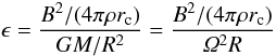 (1)be an estimate for the relative importance of the curvature force at the midplane if the rotation is Keplerian. Taking the curvature radius rc to be of the order of the disk’s scale height H and estimating Ω2 with
  (thin disk approximation), we find ϵ ~ δ/β. For β ≳ 1 and a small aspect ratio δ = H/R, the curvature force has only minor significance. It perturbs the radial equilibrium of a Keplerian disk only slightly. This difference is important, however, for the launching of the magnetically powered wind (Ogilvie & Livio 1998).
3. Methods
We use the shearing box approach (e.g., Hawley et al. 1995) with axisymmetry to solve the magnetohydrodynamic (MHD) equations in a Cartesian box that rotates with Keplerian angular velocity  at some distance R0 from the axis of rotation. Compared to the dimensions of the box, R0 is assumed to be large enough that the equations to be solved become independent of it.
List of simulations and mean properties in the evolved state.
The majority of simulations was done assuming ideal MHD, for which the induction equation has the usual form ∂tB = ∇ × (v × B). The momentum equation is 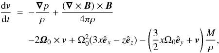 (2)where x = R − R0 is the radial coordinate and z is the height (vertical) coordinate, z = 0 corresponding to the midplane. The first two terms after the Lorentz force are the result of a Taylor expansion of the centrifugal force
  and the gravitational acceleration
  , assuming that |x|,|z| ≪ R0. The last term accounts for the momentum of material added through a mass source term (described below). We also calculated diffusive cases in which the induction and momentum equations are extended by η∇2B and ν∇2v, respectively.
To prevent the box from being drained by the outflow, we introduce a mass source term on the right-hand side of the continuity equation: 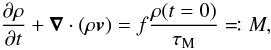 (3)where f = 1 for |z| < 0.5, f = cos [π(|z| − 0.5)] for 0.5 < |z| < 1 and f = 0 for |z| > 1. Integrated in z, the material introduced in the time span τM amounts to ΣM/Σ0 = 61% of the surface density in the initial state. It is given the initial temperature and Keplerian momentum (terms with M in Eqs. (2) and (4)). It damps horizontal and vertical motions and stabilizes the temperature.
We adopt an ideal gas equation of state with γ = 5/3 and evolve the equation for the internal energy density e = p/(γ − 1), 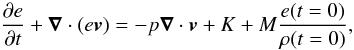 (4)along with the corresponding equation for conservation of total energy. In places where the latter yields unphysical results (“negative pressures” due to discretization errors, which occur occasionally in very low-β regions), we use the value obtained by evolving the internal energy instead of the total energy. The last term in Eq. (4)accounts for the material that is added through the mass source term. Since a calculation can become unfeasible if regions with extremely low density develop, we add another artificial source term
  (5)to the energy equation. This intervention helps to avoid low-density cavities by relaxing the temperature to that of the initial state on an appropriate time scale τK. In nature, radiative losses would prevent excessive temperatures.
3.1. Boundary conditions
We assume reflective symmetry at the midplane. The computational domain is −Lx < x < Lx in the horizontal direction and 0 < z < Lz in the vertical direction. The bottom boundary corresponds to the accretion disk’s midplane. There, we use reflective boundary conditions: ∂(ρ,T,v [x,y] ,|vz|,|B [x,y] |)/∂z = 0, the signs of vz and B [x,y] are reversed, and Bz follows from solenoidality.
The horizontal boundaries are strictly periodic for all quantities except the azimuthal velocity, for which  (6)is applied in the ghost cells of the left (right) boundary.
3.1.1. Top boundaries
The top boundary conditions (z > Lz) must account for the effects of a global magnetic field outside the scope of the local simulation and allow for an unhindered outflow of material. We tried different ways of implementing these constraints and found many to be unfit: zero-slope conditions in the vertical direction create numerical instabilities, while rigorously imposing the poloidal field inclination angle causes significant reflections, in some cases strongly affecting the dynamics in the simulated domain.
The conditions described below are constructed in view of the limiting case far above the midplane. There, β ≪ 1, which suggests that the magnetic field is force-free, and the characteristics of MHD waves along the field are outwards, which suggests the use of extrapolation along the magnetic field. A convenient assumption then is that the poloidal magnetic field is a potential one1. An inclination angle is imposed by choosing the value of the mean field. This gives the field more freedom than a strict imposition of the inclination angle. These boundary conditions work very well, even in cases where the boundary is not far in the β ≪ 1 domain and still inside the Alfvén surface. They are numerically stable and cause only minimal reflective artifacts.
The conditions are implemented as follows. At each time step, we determine the potential field that matches with Bz at z = Lz and satisfies [∇ × B] y = 0. The solution is found by means of a discrete Fourier transform in x-direction, using  for the complex Fourier coefficients of Bx (
 being the coefficients of Bz) for k ≠ 0. The mean field (corresponding to k = 0) is chosen such that at infinity the poloidal field is inclined by an angle ι with respect to the horizontal. We use zero-slope conditions along the magnetic field: with s measuring distance along a poloidal field line, ∂(ρ,v [x,y,z] ,By)/∂s = 0 to first order (i.e., the values are constant along a field line). In addition, we dismiss inertial and gravitational forces parallel to the magnetic field in the uppermost layer of cells next to the upper boundary. The temperature is kept fixed at the top boundary, ∂T/∂t = 0.
3.2. Initial conditions
The gas is initially isothermal, with both pressure and density being ∝ ![Mathematical equation: \hbox{$\exp[-z^2/(2l_0^2)]$}](/articles/aa/full_html/2012/12/aa18249-11/aa18249-11-eq186.png) , where l0 is the unit length (i.e., l0 is the scale height in the initial state; we denote the actual, time-dependent scale height of the disk with H). The initial magnetic field is homogeneous and inclined by an angle ι with respect to the midplane. Its strength is determined by the simulation parameter βi, which represents the ratio of the gas-to-magnetic pressure at the midplane in the initial state. The initial velocity is Keplerian2 at the midplane, vy = −3/2xΩ0, and constant along the magnetic field lines.
, where l0 is the unit length (i.e., l0 is the scale height in the initial state; we denote the actual, time-dependent scale height of the disk with H). The initial magnetic field is homogeneous and inclined by an angle ι with respect to the midplane. Its strength is determined by the simulation parameter βi, which represents the ratio of the gas-to-magnetic pressure at the midplane in the initial state. The initial velocity is Keplerian2 at the midplane, vy = −3/2xΩ0, and constant along the magnetic field lines.
 |
Fig. 1 Visualization of the wind properties listed in Table 1. Each “flower” represents a simulation. The radii of the “petals” are proportional to the represented value. All values are normalized by the respective value in run β1ι45. Strong clumps develop in the cases to the left and above the dotted line (cf. Figs. 4–6). Note that the β in the simulation identifiers refers to the initial state and measures the absolute field strength, whereas the β represented by the gray petals refers to the actual value in the evolved state (see Table 1 and text). |
 |
Fig. 2 Horizontal means of the surface density (green line), scale height (blue line), mass inflow rate (red line), vertical mass flux (cyan line), Reynolds stress (brown line), and Maxwell stress (purple line) as functions of time in run β1ι45. |
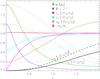 |
Fig. 3 Vertical stratification of the disk in run β1ι45: density (green line), plasma-β (blue line), sound speed (∝ square root of temperature, red line), slow magnetosonic cusp speed (cyan line), poloidal Alfvén velocity (brown line), and azimuthal magnetic field (magenta line). The solid and dashed black lines represent the vertical velocity and the velocity along the poloidal magnetic field, respectively. The curves represent the mean over the horizontal direction and time in the evolved state. For comparison, dotted lines represent the isothermal, Gaussian stratification of the initial condition (in arbitrary normalization). |
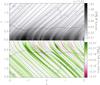 |
Fig. 4 Snapshot of the density (black/white) and the field-parallel mass flux (green/pink colors) in run β1ι45. Selected magnetic field lines are drawn in blue. The additional solid and dashed lines indicate the scale height and the sonic surface, respectively. A complementary movie is available online. |
3.3. MHD code
The simulations were performed with the Eulerian MHD code of Obergaulinger (2008). It is based on a flux-conservative finite-volume formulation of the MHD equations and a constraint transport scheme that maintains a divergence-free magnetic field (Evans & Hawley 1988). Using high-resolution shock-capturing methods (e.g., LeVeque 1992), it allows a choice of various optional high-order reconstruction algorithms and approximate Riemann solvers based on the multi-stage method (Toro & Titarev 2006). The simulations presented here were performed using a fifth-order monotonicity-preserving reconstruction scheme (Suresh & Huynh 1997), the HLL Riemann solver (Harten 1983), and third-order Runge-Kutta time stepping.
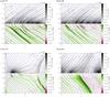 |
Fig. 5 Snapshots of the density (black/white) and the field-parallel mass flux (green/pink colors) in the evolved state of simulations with different values for the asymptotic field inclination: a) ι = 37°, b) ι = 40°, c) ι = 50°, d) ι = 60°. The ι = 45° case is shown in Fig. 4. The plots include selected magnetic field lines, the scale height (solid horizontal lines), and the sonic surface (dashed lines). |
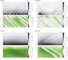 |
Fig. 6 Snapshots of the density (black/white) and the field-parallel mass flux (green/pink colors) in the evolved state of simulations with different values for the initial gas-to-magnetic pressure: a) βi = 0.5, b) βi = 2, c) βi = 8, d) βi = 10. The βi = 1 case is shown in Fig. 4. The plots include selected magnetic field lines, the scale height (solid horizontal lines), and the sonic surface (dashed lines). |
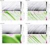 |
Fig. 7 Snapshots of the density (black/white) and the field-parallel mass flux (green/pink colors) in the evolved state of variants of run β1ι45 shown in Fig. 4. The panels show the effect of a) a bigger computational box, b) a doubled resolution, c) a doubled resolution and explicit shear viscosity, d) a doubled resolution and explicit magnetic diffusivity. The plots include selected magnetic field lines, the scale height (solid horizontal lines), and the sonic surface (dashed lines). |
4. Results
We performed several simulations with varying physical and numerical parameters. Long-lived runs, in which the disk evolution could be followed over many orbits past an initial transient, are listed in Table 1. The time scale τK for the temperature control was always taken to be 0.1 orbits, so that large deviations from the initial isothermal state are rare; e.g., in run β1ι45, only about 4% of the volume deviates from the initial temperature by more than 10%. Unless noted otherwise, the time scale τM for the mass source used was two orbits (=2π/Ω0 ≡ t0, used as unit time). In a simulation similar to β1ι45 but without a mass source (τM → ∞), the mass inside the box is diminished by 58% during two orbits (after which the increased Alfvén velocities make it impractical to continue the simulation). The material introduced with the τM = 2 mass source is roughly of this value (cf. ΣM/Σ0 in Sect. 3). The simulations were continued to ~20 orbits, at which time the system has passed through the initial transient and has entered a (more or less, depending on the parameters) quasi-stationary state.
The two basic simulation parameters are βi, which determines the strength of the magnetic field, and ι, which determines the asymptotic inclination of the poloidal magnetic field in the disk’s magnetosphere. The parameter βi is usually smaller than the mean value of β at the midplane in the evolved state, which is listed in the fourth column of Table 1. An exception are disks with very weak magnetic fields, see Sect. 4.5.
Figure 2 shows the evolution of horizontally averaged quantities in run β1ι45. In general, the simulations start with strong epicyclic oscillations in the inflow rate, presumably governed by the interplay of magnetic curvature forces (due to the bending of the magnetic field at the midplane, see Sect. 2.1), the Coriolis force, and the loss of angular momentum by the magnetically powered wind. The disk gradually enters a new equilibrium state with a vertical outflow. For further analyses, we consider only the times after the initial transient. Depending on the simulation, the evolved state is more or less relaxed. In some cases, the oscillations are still strong after many orbits (see fluctuations given in percent in Table 1), with no decreasing trend at the end of the simulated time span.
The green curve in Fig. 2 shows the surface density Σ = ∫ρ dz, normalized by its initial value. We consider it a measure for the efficiency of the wind, with strong winds yielding a smaller Σ. In the evolved state, the mass loss through the wind is balanced by the mass source, so that Σ ≈ const. The blue curve shows the scale height H, which we define here as the height that contains 68% of the mass (we take into account the finite vertical size of the computational box, so that H ≡ l0 in the initial state). The cyan curve shows the vertical mass flux near the upper boundary, measured at height z = 1.7. In the evolved state, its mean value equals the amount of material that is introduced by the mass source: ρvz ≈ ΣM/τM = 0.0676 ΣΩ0. The brown and purple lines show the Reynolds stress ρvzΔvy, where Δvy denotes the deviation from the Keplerian rotation velocity and the Maxwell stress −BzBy/4π, respectively. The red curve shows the mass inflow rate ṁin = ∫ρvx dz, normalized such that it gives, in units of the scale height, the horizontal width of the disk material that crosses a surface of constant radius per radian rotation.
Figure 3 shows (horizontally averaged) vertical profiles of various quantities in run β1ι45. Density and plasma-β, represented by the green and the blue line, decrease by factors of 15 and 50, respectively, from the midplane to the upper boundary. Both quantities drop considerably faster with height than in a Gaussian stratification. The mean of the sound speed, represented by the red line, is close to the initial value (which is  ) at every height. Above the disk, it approximates the slow magnetosonic cusp speed vc, given by
  and represented by the cyan line. The Alfvén velocity of the poloidal field, vAp, is represented by the brown line; it is by a factor of four larger than the cusp speed at the upper boundary. The magenta line represents the azimuthal magnetic field component, normalized by the vertical field (the mean of which is a constant).
Figure 4 shows snapshots of the density ρ (in units of the initial value at the midplane) and of the mass flux ρv ∥ in the direction of the poloidal magnetic field (v ∥ is computed from vz and the local field inclination) in run β1ι45. The outflow is inhomogeneous, the mass flux varies across different field lines. Dark-green stripes indicate the regions where the wind is strongest. Along some of the field lines, there is an inflow at low heights (pink colors). As angular momentum is lost through the wind, an accretion flow drags the magnetic field inward (i.e., in −x-direction). A time animation shows that the stripes move inward with the magnetic field. On a given field line, the strength of the wind varies periodically with a frequency of ~1.2 per orbit.
4.1. Dependence on field strength and inclination
The temporal means of the quantities discussed above are listed in Table 1 for different simulations. A graphical representation of these numbers can be found in Fig. 1. Snapshots of simulations with different values for the asymptotic poloidal field inclination ι are collected in Fig. 5, and those with different values of βi are collected in Fig. 6.
With increasing field inclination ι, the strength of the wind, as measured by the value of the surface density Σ or the density-normalized mass flux ρvz, decreases. The disk is less compact (increasing H) and the inflow rate smaller. The disks in runs with high inclination, ι = 50° and ι = 60°, develop a large-scale instability in the form of a density clump. We discuss the clump in the ι = 50° case in Sect. 4.4.
With increasing βi (decreasing field strength), Σ decreases; hence the wind becomes more effective at removing disk material. The inflow rate ṁin, however, is smaller. While the Reynolds stress increases, the inflow rate and the Maxwell stress, which is the dominant agent for the removal of angular momentum, both decrease. The wind is more homogeneous across the magnetic field in the high-β cases.
The mean value of β at the midplane is usually higher than the initial value βi as a result of the arbitrary initial transient. For equal asymptotic inclinations ι, the field inclination as a function of height is different in simulations with different field strengths. For instance, in run β8ι45, the horizontal separation between the foot point of a field line at the midplane and the intersection point of the same field line at the upper boundary is typically larger than in run β1ι45, see Figs. 5a and 6c. That is, the mean inclination of the field is higher in run β8ι45. In general, the inclination is a function of the field line as well as height (or distance along the field line).
4.2. Resolution, diffusion, and box size
A comparison of simulations β1ι45 and β1ι45h, Figs. 4 and 7b, shows that the inhomogeneities (stripes) in the mass flux are narrower at higher resolution. The short wavelengths appear to grow fastest, with numerical resolution the limiting factor.
We study the effects of diffusion of magnetic field and momentum through a high-resolution simulation (β1ι45hη) with an explicit magnetic diffusivity  (=
(= with cs0 = (p0/ρ0)1/2 being the isothermal sound speed in the initial state) and another high-resolution simulation (β1ι45hν) with an explicit shear viscosity
  . In the case with magnetic diffusivity, Fig. 7d (β1ι45hη), the stripes are broader than in the low-resolution simulation without diffusivity. In the case with viscosity, Fig. 7c (β1ι45hν), the wind inhomogeneities are mostly gone, but the disk develops a clump. The disk is also more affected by instabilities in a simulation with a bigger domain (β1ι45b), see Fig. 7a. The mean wind properties, however, are similar in all these cases, see Fig. 1. We conclude that the amplitude of the instability increases with length scale, with its shortest length scale limited by (real or numerical) diffusion, and its largest length by the box size.
4.3. Replenishment of mass
In the simulations presented above, the value of τM is always two. In addition to facilitating the comparison, this makes practical sense because it keeps the surface density at values that are not very far from the initial state (that of a classical thin disk). Since the mass source is somewhat artificial, it is reasonable not to have it too strong, where “strong” means putting in more mass than what would be lost without it in the course of a few orbits. On the other hand, simulations with very low density are unfeasible for numerical reasons.
Average value of the surface density Σ [Σ0] in runs with different τM.
Table 2 shows how the surface density changes for different values of the τM. As expected, it increases with decreasing τM. Considering runs with different field strengths and inclinations, Σ varies in the same direction for every value of τM.
With increasing values of τM, the solutions become more unstable, developing the typical stripes and clumps. Figure 8 shows this for the standard case. Because an increase of τM leads to a decrease of density and gas pressure, this is consistent with the observation that the amplitude of the instability increases at low β.
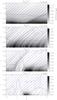 |
Fig. 8 Snapshots of the density in runs with βi = 1 and ι = 45° for different values of τM. The second panel from the top shows the standard case (β1ι45, compare Fig. 4). The solid and dashed lines indicate the scale height and the sonic surface, respectively. |
 |
Fig. 9 Snapshot of run β1ι50 during the formation of the clump. Left panel: density (black/white) and field-parallel mass flux (green/pink colors). Right panel: azimuthal velocity (sub-Keplerian in blue and super-Keplerian in red) and azimuthal inclination of the magnetic field (brown/turquoise colors). The horizontal velocity, as measured in a frame moving with the mean velocity at the midplane, is visualized with small wedges whose areas are proportional to the velocity modulus. Selected magnetic field lines and the disk’s scale height are overplotted in blue. See Fig. 5c for a snapshot in the evolved state. Two complementary movies are available online. |
4.4. Clumpy disks
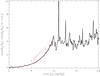 |
Fig. 10 Growth of the clump in run β1ι50. As a measure for the “clumpiness”, we use the range of poloidal field inclinations at a fixed height in the disk. |
 |
Fig. 11 Evolution of various quantities along two different field lines a) and b) in run β1ι50. From top to bottom: rotation velocity minus Keplerian value, mass flux, density, field inclination in azimuthal direction and field inclination in horizontal direction. |
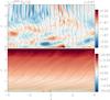 |
Fig. 12 Snapshots of the azimuthal velocity (sub-Keplerian in blue and super-Keplerian in red colors) and magnetic field lines (green) in two simulations with βi = 100: ι = 90° in the top panel and ι = 45° in the bottom panel. The initial azimuthal velocity was perturbed with white noise in both cases. |
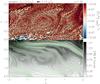 |
Fig. 13 Snapshots of velocity, density, and magnetic field lines in a simulation that begins in the evolved state of run β1ι45 (Fig. 4) but with the magnetic field strength reduced by a factor ten. Wedges depict the poloidal velocity in a frame moving with the mean horizontal velocity ⟨ vx ⟩ = −3.8 l0/t0. Red and blue colors represent super and sub-Keplerian azimuthal velocities, respectively. Two complementary movies are available online. |
In some simulations, strong horizontal inhomogeneities in the density develop: the disk condenses into one or several persistent “clumps”. A single distinctive clump forms in run β1ι50, see Fig. 5c. During the formation, the outward mass flux is often higher along field lines that are not anchored in the clump, see Fig. 9. The clump’s rotation is relatively slow (sub-Keplerian). In its wake, plasma-β is high and the field at low heights is highly inclined towards the midplane.
We measure the growth of the clump by considering the inhomogeneity of the inclination of the poloidal magnetic field inside the disk at a height of z = 0.3 ≈ 0.4 ⟨⟨H⟩⟩ . The result is depicted in Fig. 10. The perturbation grows exponentially with a growth time of 2.5 orbits. Saturation is likely influenced by the horizontal periodicity of the computational domain. In simulation β0.5ι45, which also develops a single clump, we measure an exponential growth time of 4.2 orbits by the same method.
Figure 11 shows the evolution of various quantities (a) along a field line for which the density at low heights decreases during clump formation and (b) along a field line for which the density increases. The difference in density relates to an overall stronger mass flow (green colors) along field line (a). Line (b) develops a strong twist By/Bz and a high inclination towards the midplane at low heights. Rightwards-inclined stripes in the mass flux plot indicate outward moving perturbations in the outflow. There are also fan-shaped features, which indicate perturbations that move down from the top and are reflected at the midplane.
4.5. Weak magnetic fields and MRI
The upper magnetic boundary conditions, viz., a potential poloidal field, are introduced under the assumption of strong magnetic fields with β ≪ 1. In the initial stratification, β = 1 at z = 0 in run β1ι45 and β = 1 at z = 2.1 (i.e., slightly above the upper boundary) in run β10ι45, which is the simulation with the weakest field of all cases presented above. The respective values for ⟨⟨p⟩⟩/⟨⟨pmag⟩⟩ in the evolved state are z = 0.32 and z = 0.44; both are well below the upper boundary. That is, with the exception of perhaps an initial transient, the boundary conditions are physically sound in the cases presented above.
The orderliness of the magnetic field is destroyed if the system is subject to MRI. As expected, we see such cases in simulations with very low field strengths. Figure 12 shows snapshots of two simulations with βi = 100 and no mass source (τM → ∞). In both runs, the initial azimuthal velocity vy was modified by random perturbations with an amplitude of 1 cs0 ≈ 6.3 l0/t0. In the first case (top panel), ι = 90°. The initially vertical magnetic field is radially stretched by axisymmetric MRI modes (compare, e.g., Stone & Gardiner 2010). The perturbations grow strong within roughly one orbit. In the second case (bottom panel), ι = 45°. The magnetic field becomes very flat at low heights and the density develops a strong peak: ⟨ ρ(z = 0) ⟩/⟨ ρ(z = 0.3) ⟩ ≈ 12 at t = 0.97. The field then reconnects at the midplane.
Runs with ι = 45° and βi = 12,100,1020 are all numerically unstable (i.e., some values become too extreme for the numerical solver) and terminate after ~1/2 orbit. Common to all these cases is that the magnetic field becomes very flat near the midplane. Unlike in the low-β cases, the reflecting condition does not make the field vertical near z = 0. For βi → ∞ (no magnetic field), as expected, the disk is stationary and does not generate a wind.
To test whether the peculiar behavior at very weak magnetic field strengths is tied to the initial state, we continued simulation β1ι45 with the magnetic field strength reduced by a factor ten. A snapshot of this run is shown in Fig. 13. Due to the changed magnetic forces, the originally stable system is out of equilibrium and oscillates. The magnetic field is distorted by instabilities at all heights. After about one orbit, an elongated magnetic structure develops near the midplane, moving inward fast. The mean plasma-β is smaller than 1 for z ≳ 1.35, i.e., the potential condition at the upper boundary is still practical in this simulation.
5. Summary and discussion
We have presented simulations of magnetocentrifugally accelerated winds in an axisymmetric shearing box. The box contains a thin disk with an ordered poloidal magnetic field that is inclined away from the rotation axis. Special upper boundary conditions were used that allow a study of the coupling between the disk and the angular momentum removing outflow.
For magnetic fields that are strong enough to suppress MRI, we find that material is efficiently accelerated away from the disk. To be able to follow the disk evolution over many orbits, we replace lost material by a time-independent mass source. After several orbits, the wind enters a quasi-steady equilibrium with the mass source. The strength of the wind, as measured by how efficiently it limits the amount of material in the box in spite of a constant resupply, increases with smaller magnetic field strengths or smaller asymptotic inclinations of the poloidal magnetic field. Angular momentum is lost mainly through magnetic torques (Maxwell stresses). The disks develop a radial inflow with sub-Keplerian rotation velocities near the midplane.
In general, the outflows are not homogeneous and the magnetic field lines are not uniform. All cases develop instabilities in the mass flux on the shortest length scales that are numerically resolved. In some cases, these simply saturate. In other cases, the nonlinear development is much more dramatic, leading to the formation of inward-moving density clumps. Cases with high relative field strengths (low plasma-β) develop especially strong clumps. Such a clump grows exponentially with a growth time of a few orbits. The growth is tied to inhomogeneities in the strength of the outflow along different magnetic field lines. It is accompanied by a nose-shaped deformation of the magnetic field, with the clump located at the tip of the nose. Such a massive instability has been proposed before in a simpler model of the disk-flow connection (Agapitou 2000). Clumps may be a reason for the variability detected in observations of accreting systems, for instance, the hard state noise in X-ray binaries (e.g., Lin et al. 2000).
At very low field strengths, the solutions become very different. “Classical” axisymmetric MRI modes develop if the field is vertical. The modes grow strong within roughly one orbit. With an inclined field and despite reflective symmetry, the field tends to become extremely flat near the midplane. This then leads to magnetic reconnection.
A major constraint of the simulations presented here is that 3D effects are ignored. How do the 2D stripes in the wind turn into 3D structures? We circumvented the problem of how the material lost in the outflow is replenished. In reality, this is presumably achieved through 3D interchange processes. As suggested by 3D simulations of magnetically arrested accretion flows (Narayan et al. 2003; Igumenshchev 2008), it is likely that high-amplitude clumps also form in the 3D case. This would also provide justification for the clumpy accretion of magnetic flux proposed by Spruit & Uzdensky (2005).
Online material
Movie of Fig. 4 Access Supplementary Material
Movie 1 of Fig. 9 Access Supplementary Material
Movie 2 of Fig. 9 Access Supplementary Material
Movie 1 of Fig. 13 Access Supplementary Material
Movie 2 of Fig. 13 Access Supplementary Material
However, this may not be a good approximation in cases where the azimuthal field exerts strong Lorentz forces perpendicular to the poloidal field.
Taking magnetic support against gravity (Sect. 2.1) into account would change vy by a constant amount −ϵR0Ω0/2. We opted not to include such a correction and let the system find an equilibrium by itself instead.
Acknowledgments
The author thanks Henk Spruit for his time and support of this work, and Martin Obergaulinger for providing his extremely versatile MHD code Aenus. He thanks Robert Cameron for his advice on Fourier transforms and kindly acknowledges support through the Feodor Lynen Research Fellowship by the Alexander von Humboldt Foundation.
References
- Agapitou, V. 2000, Ph.D. Thesis, Astronomy Unit, Queen Mary and Westfield College, London [Google Scholar]
- Balbus, S. A. 2003, ARA&A, 41, 555 [NASA ADS] [CrossRef] [Google Scholar]
- Balbus, S. A., & Hawley, J. F. 1991, ApJ, 376, 214 [NASA ADS] [CrossRef] [Google Scholar]
- Bisnovatyi-Kogan, G. S., & Ruzmaikin, A. A. 1976, Ap&SS, 42, 401 [NASA ADS] [CrossRef] [Google Scholar]
- Blandford, R. D. 1976, MNRAS, 176, 465 [NASA ADS] [Google Scholar]
- Blandford, R. D., & Payne, D. G. 1982, MNRAS, 199, 883 [NASA ADS] [CrossRef] [Google Scholar]
- Campbell, C. G. 2009, MNRAS, 392, 271 [NASA ADS] [CrossRef] [Google Scholar]
- Cao, X., & Spruit, H. C. 2002, A&A, 385, 289 [NASA ADS] [CrossRef] [EDP Sciences] [Google Scholar]
- Evans, C. R., & Hawley, J. F. 1988, ApJ, 332, 659 [Google Scholar]
- Fromang, S., & Stone, J. M. 2009, A&A, 507, 19 [NASA ADS] [CrossRef] [EDP Sciences] [Google Scholar]
- Harten, A. 1983, J. Comput. Phys., 49, 357 [NASA ADS] [CrossRef] [MathSciNet] [Google Scholar]
- Hawley, J. F., & Krolik, J. H. 2002, ApJ, 566, 164 [NASA ADS] [CrossRef] [Google Scholar]
- Hawley, J. F., Gammie, C. F., & Balbus, S. A. 1995, ApJ, 440, 742 [NASA ADS] [CrossRef] [Google Scholar]
- Igumenshchev, I. V. 2008, ApJ, 677, 317 [NASA ADS] [CrossRef] [Google Scholar]
- Königl, A., & Wardle, M. 1996, MNRAS, 279, L61 [NASA ADS] [CrossRef] [Google Scholar]
- LeVeque, R. J. 1992, Numerical Methods for Conservation Laws, 2nd edn., ETH Zürich: Lectures in mathematics (Birkhäuser) [Google Scholar]
- Lin, D., Smith, I. A., Liang, E. P., et al. 2000, ApJ, 532, 548 [NASA ADS] [CrossRef] [Google Scholar]
- Lubow, S. H., Papaloizou, J. C. B., & Pringle, J. E. 1994, MNRAS, 268, 1010 [NASA ADS] [CrossRef] [Google Scholar]
- Narayan, R., Igumenshchev, I. V., & Abramowicz, M. A. 2003, PASJ, 55, L69 [NASA ADS] [Google Scholar]
- Obergaulinger, M. 2008, Ph.D. Thesis, Max-Planck-Institut für Astrophysik, Garching bei München [Google Scholar]
- Ogilvie, G. I. 2012, MNRAS, 423, 1318 [NASA ADS] [CrossRef] [Google Scholar]
- Ogilvie, G. I., & Livio, M. 1998, ApJ, 499, 329 [NASA ADS] [CrossRef] [Google Scholar]
- Ogilvie, G. I., & Livio, M. 2001, ApJ, 553, 158 [NASA ADS] [CrossRef] [Google Scholar]
- Spruit, H. C., & Uzdensky, D. A. 2005, ApJ, 629, 960 [NASA ADS] [CrossRef] [Google Scholar]
- Stone, J. M., & Gardiner, T. A. 2010, ApJS, 189, 142 [NASA ADS] [CrossRef] [Google Scholar]
- Suresh, A., & Huynh, H. 1997, J. Comput. Phys., 136, 83 [NASA ADS] [CrossRef] [Google Scholar]
- Toro, E. F., & Titarev, V. A. 2006, J. Comput. Phys., 216, 403 [NASA ADS] [CrossRef] [Google Scholar]
- Turner, N. J., Stone, J. M., & Sano, T. 2002, ApJ, 566, 148 [NASA ADS] [CrossRef] [Google Scholar]
All Tables
All Figures
|
Fig. 1 Visualization of the wind properties listed in Table 1. Each “flower” represents a simulation. The radii of the “petals” are proportional to the represented value. All values are normalized by the respective value in run β1ι45. Strong clumps develop in the cases to the left and above the dotted line (cf. Figs. 4–6). Note that the β in the simulation identifiers refers to the initial state and measures the absolute field strength, whereas the β represented by the gray petals refers to the actual value in the evolved state (see Table 1 and text). |
| In the text | |
|
Fig. 2 Horizontal means of the surface density (green line), scale height (blue line), mass inflow rate (red line), vertical mass flux (cyan line), Reynolds stress (brown line), and Maxwell stress (purple line) as functions of time in run β1ι45. |
| In the text | |
|
Fig. 3 Vertical stratification of the disk in run β1ι45: density (green line), plasma-β (blue line), sound speed (∝ square root of temperature, red line), slow magnetosonic cusp speed (cyan line), poloidal Alfvén velocity (brown line), and azimuthal magnetic field (magenta line). The solid and dashed black lines represent the vertical velocity and the velocity along the poloidal magnetic field, respectively. The curves represent the mean over the horizontal direction and time in the evolved state. For comparison, dotted lines represent the isothermal, Gaussian stratification of the initial condition (in arbitrary normalization). |
| In the text | |
|
Fig. 4 Snapshot of the density (black/white) and the field-parallel mass flux (green/pink colors) in run β1ι45. Selected magnetic field lines are drawn in blue. The additional solid and dashed lines indicate the scale height and the sonic surface, respectively. A complementary movie is available online. |
| In the text | |
|
Fig. 5 Snapshots of the density (black/white) and the field-parallel mass flux (green/pink colors) in the evolved state of simulations with different values for the asymptotic field inclination: a) ι = 37°, b) ι = 40°, c) ι = 50°, d) ι = 60°. The ι = 45° case is shown in Fig. 4. The plots include selected magnetic field lines, the scale height (solid horizontal lines), and the sonic surface (dashed lines). |
| In the text | |
|
Fig. 6 Snapshots of the density (black/white) and the field-parallel mass flux (green/pink colors) in the evolved state of simulations with different values for the initial gas-to-magnetic pressure: a) βi = 0.5, b) βi = 2, c) βi = 8, d) βi = 10. The βi = 1 case is shown in Fig. 4. The plots include selected magnetic field lines, the scale height (solid horizontal lines), and the sonic surface (dashed lines). |
| In the text | |
|
Fig. 7 Snapshots of the density (black/white) and the field-parallel mass flux (green/pink colors) in the evolved state of variants of run β1ι45 shown in Fig. 4. The panels show the effect of a) a bigger computational box, b) a doubled resolution, c) a doubled resolution and explicit shear viscosity, d) a doubled resolution and explicit magnetic diffusivity. The plots include selected magnetic field lines, the scale height (solid horizontal lines), and the sonic surface (dashed lines). |
| In the text | |
|
Fig. 8 Snapshots of the density in runs with βi = 1 and ι = 45° for different values of τM. The second panel from the top shows the standard case (β1ι45, compare Fig. 4). The solid and dashed lines indicate the scale height and the sonic surface, respectively. |
| In the text | |
|
Fig. 9 Snapshot of run β1ι50 during the formation of the clump. Left panel: density (black/white) and field-parallel mass flux (green/pink colors). Right panel: azimuthal velocity (sub-Keplerian in blue and super-Keplerian in red) and azimuthal inclination of the magnetic field (brown/turquoise colors). The horizontal velocity, as measured in a frame moving with the mean velocity at the midplane, is visualized with small wedges whose areas are proportional to the velocity modulus. Selected magnetic field lines and the disk’s scale height are overplotted in blue. See Fig. 5c for a snapshot in the evolved state. Two complementary movies are available online. |
| In the text | |
|
Fig. 10 Growth of the clump in run β1ι50. As a measure for the “clumpiness”, we use the range of poloidal field inclinations at a fixed height in the disk. |
| In the text | |
|
Fig. 11 Evolution of various quantities along two different field lines a) and b) in run β1ι50. From top to bottom: rotation velocity minus Keplerian value, mass flux, density, field inclination in azimuthal direction and field inclination in horizontal direction. |
| In the text | |
|
Fig. 12 Snapshots of the azimuthal velocity (sub-Keplerian in blue and super-Keplerian in red colors) and magnetic field lines (green) in two simulations with βi = 100: ι = 90° in the top panel and ι = 45° in the bottom panel. The initial azimuthal velocity was perturbed with white noise in both cases. |
| In the text | |
|
Fig. 13 Snapshots of velocity, density, and magnetic field lines in a simulation that begins in the evolved state of run β1ι45 (Fig. 4) but with the magnetic field strength reduced by a factor ten. Wedges depict the poloidal velocity in a frame moving with the mean horizontal velocity ⟨ vx ⟩ = −3.8 l0/t0. Red and blue colors represent super and sub-Keplerian azimuthal velocities, respectively. Two complementary movies are available online. |
| In the text | |
Current usage metrics show cumulative count of Article Views (full-text article views including HTML views, PDF and ePub downloads, according to the available data) and Abstracts Views on Vision4Press platform.
Data correspond to usage on the plateform after 2015. The current usage metrics is available 48-96 hours after online publication and is updated daily on week days.
Initial download of the metrics may take a while.