| Issue |
A&A
Volume 547, November 2012
|
|
|---|---|---|
| Article Number | A6 | |
| Number of page(s) | 13 | |
| Section | The Sun | |
| DOI | https://doi.org/10.1051/0004-6361/201219454 | |
| Published online | 18 October 2012 | |
Spatially resolved observations of a split-band coronal type II radio burst
1
Space Research Institute (IKI) of RAS,
Profsoyuznaya Str. 84/32,
117997
Moscow,
Russia
e-mail: ivanzim@iki.rssi.ru
2
LESIA, Observatoire de Paris, CNRS, UPMC, Université
Paris-Diderot, 5 place Jules
Janssen, 92195
Meudon Cedex,
France
3
National Institute for Space Research (INPE) and World Institute
for Space Environment Research (WISER), PO Box 515, São José dos Campos SP
12227-010,
Brazil
4
Moscow Institute of Physics and Technology (State University),
Institutskii per. 9, Dolgoprudny, 141700
Moscow Region,
Russia
Received: 23 April 2012
Accepted: 11 August 2012
Context. The origin of coronal type II radio bursts and the nature of their band splitting are still not fully understood, though a number of scenarios have been proposed to explain them. This is largely due to the lack of detailed spatially resolved observations of type II burst sources and of their relations to magnetoplasma structure dynamics in parental active regions.
Aims. To make progress in solving this problem on the basis of one extremely well observed solar eruptive event.
Methods. The relative dynamics of multithermal eruptive plasmas, observed in detail by the Atmospheric Imaging Assembly onboard the Solar Dynamics Observatory, and of harmonic type II burst sources, observed by the Nançay Radioheliograph at ten frequencies from 445 to 151 MHz, was studied for the 3 November 2010 event arising from an active region behind the east solar limb. Special attention was given to the band splitting of the burst. Analysis was supplemented by investigation of coronal hard X-ray (HXR) sources observed by the Reuven Ramaty High-Energy Solar Spectroscopic Imager.
Results. We found that the flare impulsive phase was accompanied by the formation of a double coronal HXR source, whose upper part coincided with the hot (T ≈ 10 MK) eruptive plasma blob. The leading edge (LE) of the eruptive plasmas (T ≈ 1−2 MK) moved upward from the flare region with a speed of v ≈ 900−1400 km s-1. The type II burst source initially appeared just above the LE apex and moved with the same speed and in the same direction. After ≈ 20 s, it started to move about twice as fast, but still in the same direction. At any given moment, the low-frequency component (LFC) source of the splitted type II burst was situated above the high-frequency component (HFC) source, which in turn was situated above the LE. We also found that at a given frequency the HFC source was located slightly closer to the photosphere than the LFC source.
Conclusions. Based on the set of established observational facts, we conclude that the shock wave, which could be responsible for the observed type II radio burst, was initially driven by the multi-temperature eruptive plasmas, but later transformed to a freely propagating blast shock wave. The preferable interpretation of the type II burst splitting is that its LFC was emitted from the upstream region of the shock, whereas the HFC was emitted from the downstream region. The shock wave in this case could be subcritical.
Key words: Sun: corona / Sun: flares / Sun: radio radiation / Sun: X-rays, gamma rays
© ESO, 2012
1. Introduction
It is generally accepted that coronal type II radio bursts are a signature of magnetohydrodynamic (MHD) shock waves (e.g., Zheleznyakov 1970; Wild & Smerd 1972; Nelson & Melrose 1985; Mann 1995; Cairns 2011). Nevertheless, there is a long-lasting question as to whether these shock waves are 1) blast shocks due to explosive flare energy releases or 2) piston shocks driven by eruptive magnetoplasma structures often evolving into coronal mass ejections (CMEs). Numerous observational evidence has been reported in favor of both the first and the second scenario (Nelson & Melrose 1985; Aurass 1997; Cliver et al. 1999; Vršnak & Cliver 2008; Vourlidas & Ontiveros 2009). To make progress in solving this problem, spatially resolved observations of type II burst sources at several frequencies in the lower corona (≲2 R⊙) are required. Radio observations must be supplemented by high-precision, high-cadence, multiwavelength observations of magnetoplasma structure dynamics in parental active regions. It is obvious that limb events are best suited for this purpose.
The solar flare of 3 November 2010 (C4.9 class, ≈12:10 UT), which was partially behind the east limb, is a prominent candidate to satisfy these requirements. It was accompanied by a split-band decimetric/metric type II radio burst, whose sources were well observed by the Nançay Radioheliograph (NRH; Kerdraon & Delouis 1997) in all ten working frequencies from 445 up to ≈151 MHz. An important fact is that the radio sources were observed at low altitudes between ≈0.25 R⊙ and ≈0.65 R⊙. Moreover, the Atmospheric Imaging Assembly (AIA; Lemen et al. 2012) onboard the Solar Dynamics Observatory (SDO) observed an erupting multithermal magnetoplasma structure in the lower corona ≲0.4 R⊙ (for details, see Reeves & Golub 2011; Foullon et al. 2011; Cheng et al. 2011).
The nature of the band-splitting effect, often observed in coronal and interplanetary type II bursts, is still an unsolved riddle, although several mechanisms have been proposed to explain it (see, e.g., Krueger 1979; Nelson & Melrose 1985; Vršnak et al. 2001; Cairns 2011). The first popular mechanism, initially proposed by McLean (1967), assumes the existence of two or more regions with different physical characteristics (e.g., plasma concentration) along a shock front. The second popular mechanism was proposed by Smerd et al. (1974, 1975). It suggests that the two sub-bands of a splitted coronal type II burst are due to coherent plasma radio emission simultaneously generated in the upstream and downstream regions of a shock wave. The event of 3 November 2010 gives us an opportunity to investigate this interesting and important effect, which in turn can be closely related to the entire problem of the type II bursts origin.
It should be noted that combined analysis of this type II radio burst on 3 November 2010 and associated plasma eruption was reported by Bain et al. (2012) very recently. However, Bain et al. mainly concentrated on the dynamics of the most intense type II burst sources. Our study is more focused on the band-splitting effect.
The paper is organized as follows. Analysis of the observational data is described in Sect. 2, while results of the analysis are summarized in Sect. 3. These results are discussed and interpreted in Sect. 4. Final remarks are given in Sect. 5.
2. Observations
2.1. General properties of the event
According to the Extreme Ultraviolet Imager (EUVI; Wuelser et al. 2004) onboard the STEREO-B spacecraft, which is located at a point with heliographic coordinates ≈S06E82 during the event, a bright core of the flare appeared at ≈S20E97 (i.e., ≈7° behind the east solar limb as seen from the Earth) in the NOAA AR 11121 at ≈12:00 UT. This fact will be taken into consideration later, when heights of the investigated objects above the photosphere will be estimated.
In the frame of the Geosynchronous Operational Environmental Satellite (GOES) classification, the flare was a weak X-ray event of C4.9 class. However, the charge-coupled device (CCD) detectors of EUVI were saturated in the impulsive phase of the flare. Together with the formation of a large eruptive flare loop system this suggests that the flare was actually more powerful than it seemed from the near Earth space, since much of the flare electromagnetic emission was cut off by the limb.
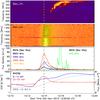 |
Fig. 1 Dynamic radio spectrograms and lightcurves of radio, soft, and hard X-ray emissions during the 3 November 2010 eruptive event. Solar radio flux density measured by the telescope in San Vito (RSTN) at 245 MHz is divided by a factor of ten for clarity. The vertical dashed line indicates the peak time (12:14:00 UT) of the hard X-ray and microwave bursts. |
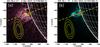 |
Fig. 2 Active area near the eastern limb of the Sun in the impulsive phase of the 3 November 2010 eruptive flare. AIA 211 Å a) and 131 Å b) base-difference images are overlaid by the RHESSI 6−12 keV (12:13:54−12:14:14 UT; light green) and 25−50 keV (12:13:54–12:14:14 UT; red) contours (20%, 40%, 60%, 80% of the peak flux), indicating locations of the flare soft and hard X-ray sources, respectively. AIA 211 Å base image was made at ≈12:00:02 UT and 131 Å base image – at ≈12:00:11 UT. Yellow ellipses are the NRH 445 MHz contours (70%, 80%, and 90% of the peak flux), which indicate the location of the decimetric radio emission source at the same moment. The thick dashed yellow straight line indicates a projection of the radius-vector passing through the centroid of the flare soft X-ray source onto the image plane. |
The light curves of the flare radio and X-ray emissions together with radio spectrograms, as observed from the Earth, are shown in Fig. 1. It is seen that the flare impulsive phase started at ≈12:13 UT and was accompanied by a burst of microwave and hard X-ray emissions with FWHM ≈ 1 min (full width at half maximum) peaking at ≈12:14 UT. The peak of the flare soft X-ray emission observed by GOES-15 was about 6 min later at ≈12:20 UT. The flare impulsive phase was also accompanied by groups of decimetric bursts (DCIM; see Fig. 4) as well as a faint type IV burst reported in Solar Geophysical Data between 12:13 UT and 12:17 UT in the 370−864 MHz range. No type III radio burst was observed during the event. This suggests that accelerated electrons have no access to open field lines. Moreover, no radio emission was observed below ≈100 MHz. The pronounced decimetric/metric type II burst was first observed at 12:14:42 UT, ≈45 s after the hard X-ray peak and until ≈12:18:00 UT.
About 20 min after the type II burst ended, a slow (vlinear ≈ 241 km s-1) and rather narrow (angular width ≈66°) CME was first detected by the Large Angle and Spectrometric Coronagraph (LASCO; Brueckner et al. 1995) at heights ≳ 1 R⊙ above the photosphere. The CME seemed to be launched from the same NOAA active region 11121 as the investigated flare. The apparent direction of CME motion was similar to those of the flare eruptive plasmas observed by the AIA in the lower corona at heights ≲0.4 R⊙.
2.2. Eruptive plasmas
2.2.1. General properties
The multithermal plasma eruption from the active region was extremely well observed by AIA above the eastern solar limb. Many aspects of these observations were already reported by Reeves & Golub (2011); Foullon et al. (2011); Cheng et al. (2011); Bain et al. (2012). Here we just point out a few main observational findings relevant to the problem of the coronal type II burst’s origin studied in our paper.
First of all, in the impulsive phase of the flare, which started at ≈12:13 UT, a hot plasma blob (plasmoid-like or flux-rope-like structure) formation and ascent (eruption) was clearly observed in the lower corona (≲0.4 R⊙) in the “hottest” AIA channels, centered on the 131 Å and 94 Å bandpasses (T ≈ 7−11 K; e.g., O’Dwyer et al. 2010; Lemen et al. 2012, Fig. 2b).
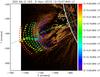 |
Fig. 3 Base-difference image of the active area near the eastern limb of the Sun made by AIA in 193 Å channel at ≈12:15:08 UT. The AIA base image was made at ≈12:00:08 UT. Dashed parabolic lines of different colors indicate the fitted LE of the eruptive plasma at an appropriate moment (see colorbar). The found parabolas’ apices are marked by squares. Green dashed straight line indicates a projection of the radius-vector passing through the flare onto the image plane (as in Fig. 2). |
Secondly, during the hot plasma blob eruption, its outer edge seemed to be wrapped with an expanding shell or rim of relatively cold (henceforth we will call it “warm”) multithermal plasmas (T ≈ 0.5−2 MK), well observed in 171, 193, and 211 Å AIA channels (Figs. 3 and 6). The thickness of this warm shell around the blob, especially above its upper (leading) edge, increased with its rise (this can be clearly seen in Figs. 6 and 8). The rising hot plasma blob (most probably, 3D flux rope in reality) appeared to push up and stretch the overlying magnetic flux tubes, causing plasma to be piled up around the blob. At the same time, some field lines seemed to tear (reconnect) beneath the blob, probably in the quasi-vertical reconnecting current sheet, thus supplying additional heat and magnetic fluxes into the blob.
Another important point is that the apparent direction of the eruptive plasma motion coincided quite well with a projection of the radial direction onto the image plane (Figs. 2, 3, 6, and 8). Finally, morphology of the parental active region, observed by EUVI during the event and by the Helioseismic and Magnetic Imager (HMI; Scherrer et al. 2011) onboard SDO spacecraft one day later, indicates that the opposite legs of eruptive arcade-like structure were situated at similar helio-latitudes. This means that most probably the eruptive structure was predominantly lying in the plane perpendicular to the image plane if observed from Earth.
The observations stated above are informatively brought together in Fig. 5 of Cheng et al. (2011). Summing up the AIA observations, the entire picture of the event was well consistent with the classical eruptive flare scenario (the so-called CSHKP model; Carmichael 1964; Sturrock 1966; Hirayama 1974; Kopp & Pneuman 1976).
2.2.2. Heights estimation technique
For our further analysis, it is of crucial importance to calculate heights of different parts of the eruptive plasmas observed in different moments as accurately as possible. We developed a special technique to calculate the hot plasma blob centroids observed in the 131 Å AIA channel (henceforth CE) and the leading edges (henceforth LE) of the hot and warm plasmas observed in the 131 Å, and 193, 211, and 335 Å AIA channels, respectively1.
First of all, for the chosen moment and AIA channel, a base-difference image is calculated with the pre-flare image at about 12:00:00 UT as a base. Then, the Lee filter is implemented on the calculated base-difference image to remove noise (Lee 1980). The Lee filter is an adaptive filter that estimates the local statistics around the chosen pixel. It preserves image sharpness and detail while suppressing noise.
The created base-difference image is divided into a set of columns that are parallel to the chosen direction. Specifically, we chose the radial direction connecting the center of the Sun and the centroid of the soft X-ray source observed by RHESSI in the pre-impulsive phase of the flare (straight dashed line in Fig. 2; see also Sect. 2.3). After this, one-dimensional scans are made along each resulting column pixel by pixel. The start of each scan is chosen at a point farthest away from the photosphere. Each scan is used to find the farthest point of the eruptive plasma LE from the photosphere. Such a point is determined when several consecutive points (e.g., N = 10, but it is not a critical parameter), if searched from the scan’s start, are strictly increasing.
For the absolute majority of all the analyzed images, the points of the LE found in the vicinity of its intersection with the chosen direction are reliably approximated by a parabola (see Figs. 3 and 7). Coordinates of the least square fit parabola’s apices are used for the further analysis (particularly in Fig. 8). Finally, the CE of the hot plasma blob in each 131 Å image is determined by averaging over coordinates of the brightness peaks of all one-dimensional scans made in the vicinity of the chosen radial direction.
The technique described above is capable of finding the position of the LE of the eruptive plasma, which is likely the LE of the magnetoplasma sheath (see Sect. 4). The technique is robust, though it could underestimate slightly (σ ≲ 15′′) the real position of the LE due to the restricted AIA sensitivity, the field of view, and the implementation of the noise supressor. The developed technique probably cannot detect the real position of the hypothetical shock wave front. However, if the shock wave front was really formed in the studied event, then it should always be situated somewhere above the estimated LE of eruptive plasmas while in the piston-driven shock wave scenario. The radio observations presented later will show some evidence in favor of this statement.
2.3. Coronal X-ray and decimetric radio sources
The initial phase of the hot plasma blob ascent (since ≈12:13 UT) was accompanied by a single impulsive hard X-ray burst with FWHM ≈ 1 min (Fig. 1). This burst was associated with the formation of a double coronal hard X-ray source (ϵγ ≈ 20−50 keV) observed by RHESSI (Fig. 2). The lower part of this double source peeped out through the limb and coincided well with the soft X-ray source in the 6−12 keV range, which was situated under the erupting hot plasma blob. At the same time, the upper part of the double source seemed to be placed inside the hot erupting plasma blob (Fig. 2). Spectral analysis of the RHESSI data reveals that the hard X-ray emission with ϵγ ≳ 20 keV was non-thermally dominated, indicating that it was produced by accelerated electrons. This is also confirmed by spectral analysis of the microwave emission (the detailed analysis will be published elsewhere). After t ≈ 12:15 UT, the upper part of the double coronal hard X-ray source disappeared on the RHESSI images, while the lower part and the soft X-ray source retained their position for several minutes. Unfortunately, it is very difficult to study reliably the dynamics of the hard X-ray sources in more detail because of the low counting rate of the RHESSI detectors at ϵγ ≳ 20 keV. Nevertheless, a connection between the coronal hard X-ray sources appearance and plasma eruption is evident.
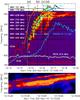 |
Fig. 4 Background-subtracted dynamic radio spectrum of the 3 November 2010 solar eruptive event obtained with the Phoenix-4 spectrograph (upper panel). Green and turquoise horizontal strokes with diamonds in the middle indicate respectively when the sources of the LFC and HFC of the type II burst’s H-component (H) were observed by the NRH for the first 10 s after its first appearance. Crosses of the same colors represent the LFC’s and HFC’s first appearence at different frequencies below 180 MHz according to the San Vito spectrograph data. Dark blue horizontal strokes with diamonds indicate the 10 s intervals of the HFC maximal intensity in appropriate frequencies. Time profiles of radio flux density measured by the NRH from the south-eastern sector of the Sun with time cadence of 1 s as well as one second solar radio flux density measured by San Vito telescope (RSTN) at 610 MHz are shown by the black and white curves, respectively. Four seconds RHESSI corrected count rates at the 6−12 and 25−50 keV ranges are depicted by the blue and red curves, respectively. The green vertical dashed line indicates the start time of the type II burst’s H-component. Black vertical dash-dotted lines marked by (a), (b), (c), (d) letters on top of the panel indicate four different moments for which four panels of Fig. 7 were made. The orange dash-dotted line connects the separated fragments of the type II burst’s F-component (F). The thin turquoise rectangular box indicates a piece of the spectrogram, which is represented in the lower panel using a slightly different color palette. The band splitting of the type II burst H-component is clearly seen. |
The hard X-ray burst was accompanied by an impulsive microwave burst (observed particularly by the San Vito telescope, a part of the Radio Solar Telescope Network, RSTN) as well as by groups of decimetric bursts with low and high frequency cut-offs at fl ≈ 400 and fh ≈ 700 MHz, respectively (marked DCIM in Fig. 4). Source centroids of these decimetric bursts were located ≈160 Mm away from the coronal hard X-ray sources and ≈110 Mm from a trajectory of erupting plasma (Fig. 2). Note that such a displacement of coronal hard X-ray sources and decimetric bursts has been reported in other events (e.g., Benz et al. 2011). This indicates that nonthermal electrons accelerated in the impulsive phase of the flare, during the eruption of plasma, could be injected into magnetic flux tubes extending to the periphery of the active region. It could be that this phenomenon has similar roots with the type II precursors reported by Klassen et al. (1999, 2003).
2.4. Type II burst
The background-subtracted dynamic radio spectrum of the Sun, obtained with the Phoenix-4 spectrograph (Bleien, Switzerland; http://soleil.i4ds.ch/solarradio/) is shown in Fig. 4 (upper panel). The bright (Imax ~ 103 SFU) type II burst with signatures of herringbone structures started about 45 s after the peak of the hard X-ray and microwave burst. Most probably, we observed mainly a second harmonic emission (denoted by “H”), whereas the type II burst at the fundamental frequencies represented only a few minor fragments or wisps (denoted by “F” and connected by orange dash-dotted line for clarity). Indeed, often in the events, especially placed far away from the disc center, metric radio emission observed at fundamental frequencies is supressed (e.g., Zheleznyakov 1970; Nelson & Melrose 1985). We will concentrate mainly on the H-component analysis.
The H-component was first observed at a high frequency of ≈561 MHz at about 12:14:43 UT (marked by green vertical dashed line in Fig. 4). It can be seen that the H-component itself is split into two sub-bands. Henceforth we will call them low and high frequency components (LFC and HFC in Fig. 4). We will call the less intense frequency band between the LFC and HFC “band gap”. The band splitting was more pronounced in the ≈200−350 MHz frequency range (see lower panel of Fig. 4) between ≈12:15:20 UT and ≈12:16:00 UT. The presence of the LFC and HFC is also confirmed by inspecting the one-second time profiles of solar radio flux density measured by the NRH; they showed two well time-separated flux increases at five NRH frequencies below 298.7 MHz (thick solid black lines on the upper panel of Fig. 4). In general, the LFC was less intense (factor of two) and had narrower frequency bandwidth (factor of 3−5) than the HFC. In turn, the gap was 2−3 times less intense than the LFC.
We estimate the mean value of the instantaneous relative bandwidth as ⟨Δf(ti)/f(ti)⟩ = ⟨ [fHFC(ti) − fLFC(ti)] /fLFC(ti)⟩ = 0.16 ± 0.02, where fLFC(ti) and fHFC(ti) is the starting frequency of the LFC and HFC, respectively. The starting frequency is taken each fifth observational moment ti (i.e., each 1 s), and the ⟨...⟩-averaging is done over all observational moments ti during the time interval ≈12:15:30−12:15:55 UT, when the LFC and HFC were best separated on the Phoenix-4 spectrogram. The value of ⟨Δf/f⟩ found is consistent with the earlier observations (e.g., Nelson & Melrose 1985; Mann 1995, and references therein). The LFC and HFC drifting rates (− df/dt) ranged from ≈1 to ≈9 MHz s-1 with a mean value of ≈2.2 MHz s-1. This value is anomalously high in comparison with the previously estimated drifting rates −df/dt ≲ 1 MHz s-1 in the majority of metric type II bursts (Nelson & Melrose 1985; Mann 1995, and references therein). However, such high values of(−df/dt) have already been reported a few times for decimetric/metric type II bursts with high starting frequencies (e.g., Vršnak et al. 2002; Pohjolainen et al. 2008).
It is very fortunate that NRH made observations of the Sun (within its field of view FOV ≈ 2° × 2°) at all ten operating frequencies (445.0, 432.0, 408.0, 360.8, 327.0, 298.7, 270.6, 228.0, 173.2, and 150.9 MHz) during the 3 November 2010 event. It should also be noted here that the flare time (at around noon in France) is most favorable for making precise observations with NRH during the day because of minimal zenith distance of the Sun. Implementing the standard technique within the SolarSoftWare to the NRH data obtained with moderate time cadence of 1 s and the half-power beam width (i.e., major axis of lobe) of ≈45′′, 46′′, 49′′, 56′′, 61′′, 67′′, 74′′, 88′′, 116′′, and 133′′ at frequencies mentioned above, respectively, we generate ten series of 128 pixel × 128 pixel 2D intensity images of solar radio emission within the entire NRH’s FOV ≈ 2° × 2°. The chosen pixel size is ≈15′′. In each image, the observed type II burst sources are well fitted by 2D Gaussians that give us estimations of the LFC and HFC source centroid positions. For better statistics at each frequency, we find source centroid positions taking an averaging over ten consecutive images at around the moment of interest to us. Specifically, we are most interested in: a) moments of the first appearance of LFC source at each of ten NRH frequencies; b) moments of the first appearance of the HFC source at five NRH frequencies 298.7, 270.6, 228.0, 173.2, and 150.9 MHz, i.e., at those NRH frequencies at which the HFC was clearly separated from the LFC by the band gap according to the Phoenix-4 spectrogram; c) moments of maximum intensity of the HFC at the same five NRH frequencies as in (b).
These three different kinds of moments are marked by green, turquoise, and dark blue horizontal strokes with diamonds on the upper panel of Fig. 4, respectively. Lengths of the horizontal strokes indicate ten-second time intervals over which averaging of the centroid positions are done at a given frequency.
The detailed comparison of the relative positions and dynamics of the LFC and HFC sources and of the eruptive plasmas observed by AIA will be done in the next subsection. Here we just compare average positions of the LFC and HFC source centroids at six NRH frequencies (327.0, 298.7, 270.6, 228.0, 173.2, and 150.9 MHz) at which the band splitting of the type II burst was best seen (see Fig. 4). The averaging is made over the entire duration of the LFC and HFC at a given frequency. Durations of the LFC and HFC are different at different frequencies. Duration of the LFC at 327.0−228.0 MHz is about 20 s, at 173.2 MHz – 25 s, and at 150.9 MHz – 40 s. Duration of the HFC at 327.0 MHz is about 16 s, at 298.7 MHz – 22 s, at 270.6 MHz – 36 s, at 228.0 MHz – 31 s, at 173.2 MHz – 30 s, and at 150.9 MHz – 40 s. Figure 5 illustrates the comparison. It is seen that at a given frequency the average position of the HFC source centroid was a little bit closer to the photosphere and the flare site than the average position of the LFC source centroid. This subtle effect may be due to large error bars, especially at the lowest NRH frequencies. However, as it is systematic at all frequencies, it may be significant and related to the origin of the band splitting (see Sect. 4.2.1 for its discussion).
It should be briefly noted here how the experimental uncertainties shown in Fig. 5 were estimated. The same principle will also be used in the next subsection (e.g., vertical bars in Fig. 8). At a given NRH frequency fi, the uncertainty is calculated (and most probably overestimated) as σ(fi) = σ1(fi) + σ2(fi) + σ3(fi). Here σ1 is the square root of dispersion of the type II burst centroid position in the given time interval, σ2 is half the image pixel diameter (i.e., σ2 ≈ 11′′ for all fi), and σ3 is a measurement of the displacement of the observed radio images with respect to the true position due to ionospheric waves. These waves with time periods of several tens of minutes are the major contributors to the errors for the absolute pointing of the NRH (Kerdraon, priv. comm.). Thus, we estimate σ3 to be approximately equal to the standard deviation of the centroid positions of a noise storm above the east limb, which was observed by the NRH at 173.2 and 150.9 MHz during the 11:00:00−12:13:00 UT time interval just prior to the flare impulsive phase. For the remaining eight frequencies, at which the noise storm was not well observed by the NRH, the errors are estimated using  rough approximation (Zheleznyakov 1970, and references therein). The contribution of σ3 is found to be the largest to the uncertainties, especially at low frequencies.
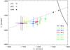 |
Fig. 5 Average positions of the type II burst’s LFC and HFC sources observed by NRH at several frequencies during the 3 November 2010 eruptive event. Error bars of the LFC and HFC source centroid estimations are shown. Positions of the double coronal hard X-ray source observed by RHESSI in the flare impulsive phase are also plotted by two black asterisks for comparison. The straight black dashed line indicates a projection of the radius-vector passing through the double coronal HXR source onto the image plane. The solar optical limb is represented by black solid arc-like line. |
2.5. Type II burst sources versus eruptive plasmas
Figure 6 illustrates the relative dynamics of the multitemperature eruptive plasmas and of the LFC source. The images are shown for the time of the first appearance of the LFC source at a given frequency (these times are marked by green horizontal strokes with diamonds in the upper panel of Fig. 4). Appropriate AIA and NRH images are close to each other within 8 s, i.e., they can be considered here as almost simultaneous. It is clearly seen that the LFC source at the highest NRH frequencies initially appeared slightly above the LE of the warm eruptive plasma and that the distance between the LFC source at lower frequencies and the LE was increasing with time. This indicates that the agent which excited the LFC source was moving faster than the LE of the eruptive plasmas. A similar situation is found for the starting moments of the HFC source, with the only difference being that it was located a little bit closer to the LE of the eruptive plasmas.
Figure 7 shows the relative positions of the LFC and HFC sources and of the eruptive plasmas at four different times indicated by vertical dash-dotted black lines and marked by (a), (b), (c), and (d), respectively, in Figs. 4 and 8. It is seen that at any given time both the LFC and HFC sources are located above the LE of the erupting plasma. Only the highest-frequency part of the HFC source at 327.0 MHz seems to be located inside the warm eruptive plasma on the panel (b). We will discuss that this could be the result of a projection effect in Sect. 4. Figure 7 also shows that at a given time the LFC sources are located above the HFC ones. This indicates the presence of a natural plasma density stratification above the erupting plasmas. Both the apex of the LE of the erupting plasma and the LFC and HFC source centroids are situated close to the projection of the radius-vector passing through the X-ray flare onto the image plane.
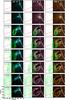 |
Fig. 6 Partial time sequence of AIA/SDO 131, 211, and 193 Å base-difference images in between 12:13:10 UT and 12:16:30 UT of 3 November 2010. Overplotted are the iso-intensity contours (50%, 60%, 70%, 80%, and 90% of the maximum) of the LFC source observed by NRH at different frequencies at a vicinity of times of its first appearance (indicated in the upper left corner of the AIA 131 Å images). One-second integrated NRH data is used. The closest AIA images in time to the NRH ones are shown (the time difference is less than eight seconds in each case). Solar limb is depicted by the thick white line. The red dashed straight line in all panels indicates a projection of the radius vector passing through the X-ray flare onto the image plane. The AIA’s field of view is less than that of the NRH. |
To investigate the relative dynamics of the multithermal erupting plasmas and of the LFC and HFC sources in more details, we built a height-time plot (Fig. 8), where we present as a function of time the heights above the photosphere of:
-
1.
apices of the LE of the warm and hot eruptiveplasmas estimated using the technique discussed inSect. 2.2.2;
-
2.
centroids of the hot erupting plasma blob;
-
3.
centroids of the LFC and HFC sources at the moments of their first appearance at different frequencies;
-
4.
centroids of the HFC sources at the moments of the maximum brightness of the HFC at different frequencies;
-
5.
centroids of the double coronal hard X-ray sources.
Calculated heights of all these objects were corrected for the location of the parental flare region behind the limb. Error bars are indicated in the plot. We also indicate here results of the least square fitting of the observational data points with a linear function. The linear approximation seems quite reasonable in this particular case. The estimated velocities of the investigated objects are summarized in the lower right-hand corner of Fig. 8 and in Table 1. It shows that the LFC source was moving approximately two times faster than the LE of the warm eruptive plasma, which in turn was moving approximately two times faster than the hot plasma blob (in good consistency with the results of Cheng et al. 2011; Bain et al. 2012). The last fact implies that the width of the apparent warm envelope around the hot plasma blob was increasing in time. The HFC source, which has a broader bandwidth than the LFC at any given time, seems to fill almost all the space between the LFC source and the LE of the warm erupting plasma. It is also worth mentioning here that the approximating curves of the LFC (start) and HFC (maximum) data points (green and dark blue straight lines in Fig. 8, respectively) intersect with the upper part of the double coronal hard X-ray source position in the height-time plot. However, it is difficult to say whether this was purely accidental or not.
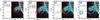 |
Fig. 7 Composite base-difference images of the active area near the eastern limb of the Sun made by AIA in 131 Å (turquoise) and 211 Å (purple) passbands at four different times of the 3 November 2010 event. These times are marked by dash-dotted vertical lines in Figs. 4 and 8. Green, yellow, and red dashed parabolas on panels a), b) and c), respectively, indicate the approximated LE of eruptive plasma observed by AIA in 211 Å passband. The parabolas’ colors are consistent with the colorbar in Fig. 3. Solid lines of different colors are the NRH contours (95% of the peak flux), which indicate locations of centroids of the type II burst sources at different frequencies (indicated within each panel) at appropriate moments. All AIA and NRH images are matched within 5 s. Red dashed line in all panels indicates a projection of the radius-vector passing through the X-ray flare onto the image plane. |
All the velocities estimated in Table 1 are probably super-magnetosonic (see also Sect. 4.2.1 on this issue) at the coronal levels where the type II burst is observed, i.e., at heights H ≈ (0.2−0.6) × R⊙ above the photosphere (this inference will be used further in Sect. 4). Indeed, the sound velocity is estimated as vs ≈ 150−220 km s-1 if the background temperature is suggested to be of reasonable coronal values T ≈ 1−2 MK. To estimate the Alfvén speed, we need first to estimate the magnetic field strength B. For this purpose, we use the rough relation B = 0.5 × H-1.5 G obtained by Dulk & McLean (1978) from radio observations. It gives B ≈ 1−6 G. Secondly, we need to estimate the electron plasma density ne. This can be done using the entire frequency band of the type II burst ≈560−130 MHz. Taking into account that the second harmonic emission was observed, we infer ne ≈ 5 × 10⁷−1 × 109 cm-3. Thus, the rough Alfvén and fast magnetosonic speed estimation is vA ≈ 310−420 km s-1 and  km s-1, respectively.
3. Results
The summary of our findings is presented below.
-
1.
The hot (T ~ 10 MK) plasma blob started to erupt in analmost radial direction in the impulsive phase of the3 November 2010 flare. Thecharacteristic velocity of the hot plasma blob upward motion wasvCE ≈ 500 km s-1.
-
2.
The hot plasma blob was surrounded by the warm (T ~ 1−2 MK) expanding rim. The characteristic velocity of the LE of this warm rim was vLE ≈ 1100 km s-1, i.e., about twice that of vCE.
-
3.
The flare impulsive phase was accompanied by the formation of a double coronal hard X-ray source. The lower part of this source seemed to coincide with the near limb legs of the erupting magnetoplasma structure, whereas the upper part was placed somewhere inside the hot erupting plasma blob.
-
4.
Half a minute after the peak of the flare impulsive phase, the type II radio burst appeared at decimetric/metric wavelengths. Mainly the second harmonic emission was observed in ≈560−130 MHz range. Signatures of herringbone structures were found, but no type III radio bursts were observed during the entire event. This suggests that accelerated electrons had no access to open magnetic field lines in the course of the plasma eruption.
-
5.
The type II burst was splitted in two sub-bands, low- and high-frequency components (LFC and HFC). The mean value of the instantaneous relative bandwidth was estimated as ⟨Δf/f⟩ = 0.16 ± 0.02. This value is within the statistics reported for the split-band coronal type II radio bursts.
-
6.
The LFC was about two times less intense and had 3–5 times narrower frequency bandwidth than the HFC.
-
7.
The LFC and HFC sources had similar circular shapes, but at a given frequency the LFC source had a slightly smaller size than the HFC one.
-
8.
Initially, the LFC source was observed by the NRH just near the apex of the warm eruptive plasma rim, but it was moving upward at twice the speed of the rim’s apex. The characteristic velocity of the LFC source was estimated as vLFC ≈ 2200 km s-1.
-
9.
The apparent direction of the LFC source motion coincided well with the radial one and that of the erupting plasma.
-
10.
At any time the HFC source seemed to fill almost all the space between the LFC source and the LE of the warm plasma rim.
-
11.
Linear back-extrapolation of the observational data points on the height-time plot gave evidence that an exciting agent of both the LFC and HFC sources could be launched from the vicinity of the upper part of the double coronal hard X-ray source in the flare impulsive phase.
Velocity estimations of different moving objects observed in course of the 3 November 2010 eruptive event.
4. Discussion
First of all, it should be noted that according to the AIA/SDO and RHESSI combined observations, the entire picture of the 3 November 2010 event was consistent with the standard eruptive flare scenario, i.e., the CSHKP model (see also Reeves & Golub 2011; Foullon et al. 2011; Cheng et al. 2011). Shock waves of various kinds are expected phenomena of such a model (e.g., Hirayama 1974; Priest 1982).
However, we shall also clarify here that there is no direct observational evidence of a shock in this event. No shock wave fronts that would have sharply separated the “disturbed” (downstream) and “undisturbed” (upstream) regions ahead of the LE of the erupting plasmas were found using EUV observations of the AIA/SDO. We emphasize that the measured LE of the eruptive plasmas is most probably not a hypothetical shock wave front. If a shock wave was indeed formed, its front should always be located somewhere above the measured LE. Nevertheless, compelling indirect evidence of a shock wave formation was found in this event with the NRH and Phoenix observations: the type II radio burst sources were observed to propagate with (probably) super-magnetosonic speeds above the LE of the eruptive plasmas. We will thus assume below that a shock wave was really formed in this event.
Our discussion will be limited to two subjects: 1) possible origin of the shock wave; 2) possible origin of the observed band splitting of the type II radio burst.
4.1. Shock wave driver
As already been mentioned in Sect. 1, type II radio bursts are believed to be produced by MHD shock waves. However, it is still unclear whether these shock waves are bow or piston shocks driven by eruptive magnetoplasma structures or blast shocks due to an explosive flare energy release localised in space and time (see comprehensive reviews on this topic given by, e.g., Vrsnak & Lulic 2000; Vršnak & Cliver 2008).
4.1.1. Piston-driven shock wave
We found strong evidence in favor of the first (piston-driven shock wave) scenario: 1) the location of the type II burst sources above the apex of the eruptive plasma LE (see Figs. 6−8), and 2) the same propagation direction of the type II burst sources and erupting plasma apex (see Figs. 3, 5, and 6).
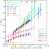 |
Fig. 8 Height-time plot of the type II burst sources observed by NRH versus different parts of the multi-temperature eruptive plasmas observed with AIA/SDO. The double coronal hard X-ray source heights observed by RHESSI in the flare impulsive phase are also plotted by orange crosses with diamonds. Black dashed and dash-dotted vertical lines indicate the beginning of the type II burst and four time moments for which panels a)–d) of Fig. 7 were created, respectively. Error bars of all object estimations are shown with vertical and horizontal strokes of appropriate colors. Heights of the type II burst’s LFC and HFC sources are given for those time intervals, which are shown by the same colors (green, turquoise, and dark blue) in Fig. 4. The least square fittings of the observational data points with the linear functions are plotted by the straight lines of appropriate colors. |
These results are similar to the results obtained by Bain et al. (2012) for the same event of 3 November 2010 and by Dauphin et al. (2006) for the 3 November 2003 flare, when the type II burst sources were observed originating above the rising soft X-ray loops. Both Bain et al. (2012) and Dauphin et al. (2006) interpreted their observations in the frame of the piston-driven shock wave scenario. Spatially resolved observations of the coronal type II burst sources in a close association with the propagating disturbances observed in the soft X-ray range were also reported earlier by, e.g., Klein et al. (1999) and Khan & Aurass (2002); it was argued that the shock waves, which could be responsible for the type II bursts, were most probably driven by these disturbances.
The fact that the estimated speed of the agent that excited the LFC source of the type II burst was much larger than the speed of the supposed driver (vLFC ≈ 2vLE ≈ 2200 km s-1), i.e. the erupting plasma, is not contradictory to the piston-driven scenario. The shock front velocity is indeed expected to be equal to the driver velocity only when the driver has a constant geometrical shape, when it propagates in a homogeneous background medium, and when the oncoming background plasma can wrap the driver’s body. A bow shock wave is formed in this case (e.g., Vrsnak & Lulic 2000). However, in the present event the possible shock driver is propagating in the stratified solar atmosphere with decreasing magnetic field and plasma density. Its geometrical size increases in time (see Fig. 6), and the upstream background plasma can not easily pass the eruptive warm plasma rim because the later seems to remain rooted to the photosphere by magnetic field lines. Thus, the driver looks like a 3D expanding piston (probably not a spherical one but rather flux-rope shaped), which also has a preferred (upward) direction of motion. A situation when a shock wave propagates through the gravitationally stratified corona including dense loops was numerically simulated, e.g., by Pohjolainen et al. (2008); Pomoell et al. (2008, 2009). It was found that under these conditions the shock wave can propagate faster through the corona than its driver (see Sect. 4.2.1 for further discussion of this issue). It was also found that the shock front is strongest near the LE of the erupting plasma.
4.1.2. Blast shock wave
Contrary to the piston-driven shock wave scenario, only one piece of indirect evidence (see Result 11 in Sect. 3) could support the second (blast shock wave) scenario. It implies that a free-propagating blast shock wave could in principle be generated by the impulsive flare energy release that was evidenced by the formation of the coronal hard X-ray sources in the flare impulsive phase. Bain et al. (2012) did not completely rule out this possibility for the present event of 3 November 2010. Vršnak et al. (2006) also reported evidence in favor of the blast shock wave scenario for the similar event of 3 November 2003. On the other hand, Result 11 may be just a coincidence. It alone seems not enough to interpret the studied type II burst in the frame of the blast shock wave hypothesis. Moreover, it is obvious that the blast shock wave hypothesis can not easily explain the same propagation direction of the type II burst sources and of the erupting plasma apex. For these reasons, we conclude that the type II burst studied here was most probably produced, at least in the initial stage, by a piston-driven shock wave rather than by a blast shock wave.
Additional comments on the assumption of the piston-driven scenario for this event are found below. The value of vLFC ≈ 2200 km s-1 was obtained using the linear least square approximation of all ten observational data points for the LFC sources (shown by green marks on the height-time plot (Fig. 8)). However, the first (in time) half of these data points in Fig. 8 seems to behave differently than the second half, thus indicating that a linear approximation is probably not the best one. If the linear approximation is performed only on the first group of data points, the slope of this linear fit line is much closer (although a little bit steeper) to the slope of the linear fit for the LE of the eruptive plasma (red and black lines in Fig. 8). This means that during the beginning of the type II burst the characteristic velocity of its sources was similar to the velocity of the eruptive plasma LE. About 20 s later, it became about twice the magnitude, i.e. vLFC ≈ 2200 km s-1.
Recent numerical simulations of Pomoell et al. (2008, 2009) have shown that the shock wave velocity can quickly exceed the velocity of the driver (flux rope) and the shock then escapes from the driver. In other words, it was found that the shock wave can be of the piston-driven type in the beginning of the eruption and, after some time, it can transform to the freely propagating blast wave. These findings of Pomoell et al. (2008, 2009) are very similar to our observations.
It should also be mentioned here that the discussed change of slope in the type II data points occurred at the time when the band splitting was first observed. It is possible that these two facts could be related to each other.
4.2. Split-band effect
It is not clear yet which physical mechanism is responsible for the splitting of the emission of type II bursts. Currently, two interpretations dominate. This does not mean, of course, that alternative ideas are not valid (e.g., Treumann & Labelle 1992; Cairns 2011, and references therein).
One popular interpretation (henceforth Scenario 1) was proposed by Smerd et al. (1974, 1975). It suggested that the two sub-bands of splitted coronal type II bursts, the LFC and HFC according to our terminology, could be due to coherent plasma radio emission simultaneously generated ahead of and behind a shock wave front, i.e., in the upstream and downstream regions, respectively.
Another popular interpretation (henceforth Scenario 2), initially proposed by McLean (1967), suggests that different parts of a shock wave front could simultaneously encounter coronal structures of different physical properties, such as electron plasma density or magnetic field. When different parts of a shock wave front propagate through the corona in more than two media with different physical conditions, observations of a type II burst with a multiple set of bands can be expected. Different situations could occur. For example, those parts of the shock front that are parallel to surfaces of constant electron density would emit more intensively in some narrow frequency ranges than in others. In particular, McLean (1967) simulated an idealized situation of a shock front encounter with a streamer and could reproduce split band of type II bursts. Similar ideas based on the shock drift acceleration mechanism have been discussed by, e.g., Holman & Pesses (1983). Recently, more sophisticated but ideologically similar numerical experiments by Knock & Cairns (2005) also reproduced splitting of coronal type II bursts.
4.2.1. Scenario 1
It seems that our observations geometrically support Scenario 1 more than Scenario 2. The major argument in favor of the upstream-downstream scenario of Smerd et al. (1974, 1975) is that LFC source is always located above the HFC one, and the HFC source fills almost all the space between the LFC source and the LE of eruptive plasmas (see Figs. 7 and 8)2. This is schematically illustrated in Fig. 9. In this case, the LFC source, situated in the upstream region, can be naturally explained in the frame of some standard shock wave theories, i.e., the shock drift acceleration mechanism.
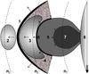 |
Fig. 9 Schematic illustration of the 3 November 2010 eruptive event observations combined with their interpretation in the frame of the upstream-downstream scenario (see text). View is from the heliographic north pole. Direction to the Earth is marked by a thick black arrow. Notations: (1) hypothetical shock wave, (2) LFC source of the type II burst, (3) its HFC source, (4) turbulent magnetosheath, (5) warm (T ≈ 1−2 MK) plasma rim and (6) its LE, (7) hot (T ≃ 10 MK) erupting flux rope or plasma blob if observed from the Earth, (8) photosphere. Thin black arrows show directions of the eruptive plasmas, shock wave, LFC and HFC sources motion. Lengths of the arrows are proportional to the corresponding velocities of motion. Levels of constant undisturbed background electron plasma concentration, assuming the natural gravitational stratification, are marked by black dashed arc-lines, and n1 > n2 > n3. |
There is another important argument in favor of Scenario 1. It was found (see Sect. 2.4 and Fig. 5) that at a given frequency the average position of the HFC source centroid was a little bit closer to the photosphere (and the flare site) than the average position of the LFC source at the same frequency. Although this is a subtle effect, it shows that at any time the plasma density in the region from where the HFC sources are emitted is enhanced relative to the undisturbed background plasma density. In our opinion, the natural explanation of this effect is that, at a given frequency, the HFC sources were emitted below the shock wave front in the downstream region, i.e., in the magnetosheath, whereas the LFC sources were emitted at the same frequency in the upstream region. This idea is schematically illustrated in Fig. 10.
Both similar and opposite behaviours of the LFC and HFC sources were reported earlier in the literature (e.g., Dulk 1970; Nelson & Robinson 1975; Aurass 1997; Khan & Aurass 2002). In some cases, the LFC sources are located farther from the flare site (or from the photosphere) than the HFC sources at the same frequencies; in other cases, however, they are closer to or almost at the same positions. All these earlier observations (known to us) were made at frequencies below ≈160 MHz or for flare regions that were located close to the center of the visible solar disk. This makes it difficult to carry out a direct analogy between these observations and our own.
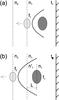 |
Fig. 10 Schematic illustration of the lower location of the HFC sources of the type II burst with respect to the LFC sources observed at the same frequency. Panel a) corresponds to an instant t1, which is before the instant t2 (t2 > t1) of panel b). Solar surface is depicted by thick black line with inclined ticks on the right. Thick dashed arc-like line shows the shock wave front. Light and dark grey ellipses represent the LFC and HFC sources, respectively. Horizontal arrow shows the direction of their movement. Levels of constant plasma density are shown by vertical straight dashed and dotted lines. Corresponding plasma densities are marked by n1, |


Scenario 1 meets, however, with a couple of difficulties. The generation of HFC emission requires intense electron plasma waves in the downstream region, whereas in situ measurements near the interplanetary shocks reveal them mainly in the upstream region (e.g., Bale et al. 1999; Thejappa & MacDowall 2000; Hoang et al. 2007; Pulupa & Bale 2008). The generation of strong Langmuir turbulence in the downstream region is not easily understood from the theoretical point of view either (e.g., Treumann & Labelle 1992; Cairns 2011). Moreover, the type II radio emission itself is also generally observed from the upstream region of interplanetary shock waves, but not from the downstream region (e.g., Reiner et al. 1998; Bale et al. 1999).
There is, however, observational evidence of radio emission coming from the downstream region of interplanetary shocks (e.g., Hoang et al. 1992; Lengyel-Frey 1992; Moullard et al. 2001). In addition, some properties of shock waves in the corona may vary from those in the interplanetary medium, while spacecraft measurements in the interplanetary space are still limited both by single point measurements and sensitivity of instrumentation. Also, the theory of collisionless shocks is still under development, and we do not fully understand them. Moreover, some suggestions that a shock front has a wavy (rippled) shape allow us to explain the downstream populations of energetic electrons even in the frame of the standard shock acceleration theory (e.g., Vandas & Karlický 2000; Lowe & Burgess 2000). Indeed, anisotropic populations of suprathermal electrons were commonly found downstream from that portion of the Earth’s bow shock where the shock normal was quasi-perpendicular to the upstream magnetic field, though suprathermal electrons sharply lost their anisotropy and fluxes with increasing penetration into the sheath (e.g., Gosling et al. 1989). This may suggest that populations of nonthermal electrons accelerated at the shock wave front could also be found in the downstream region.
It is not necessary for the nonthermal electron beams responsible for the Langmuir turbulence and the HFC radio emission in the downstream region to be accelerated directly at the shock front. Electrons could also be efficiently accelerated somewhere in the space between the shock front and the LE (or on it) of the erupting magnetoplasma structure, i.e., in the magnetosheath (Fig. 9). For example, it is known both from in situ measurements (e.g., Moullard et al. 2001; Wei et al. 2003; Gosling et al. 2007; Wang et al. 2010; Chian & Muñoz 2011) and numerical experiments (e.g., Schmidt & Cargill 2003; Wang et al. 2010) that magnetic reconnection can occur at the interface between the LE of interplanetary coronal mass ejections (ICMEs) and background solar wind magnetic field (see also Démoulin 2008). Such episodes of magnetic reconnection could supply beams of suprathermal and/or nonthermal energetic electrons to the sheath region (Wang et al. 2010; Huang et al. 2012), thus possibly creating the necessary conditions for the generation of the Langmuir turbulence and radio emission there. However, we realize (and emphasize) that this important issue requires further studies.
If the upstream-downstream scenario really takes place in the studied event, then it is possible (e.g., Smerd et al. 1974, 1975; Mann 1995; Vršnak et al. 2002) to estimate the upstream (i.e., background) magnetic field (Bu) using the density jump found at the shock front X = nd/nu ≈ nHFC/nLFC = (fHFC/fLFC)2 = (1 + ⟨Δf/f⟩)2 ≈ 1.35, and compare it with those values which were estimated in Sect. 2.5 using the formula of Dulk & McLean (1978). We will suggest here that the shock wave was oblique rather than purely parallel or perpendicular because a slightly oblique (quasi-perpendicular) shock wave seems to be a more favorable accelerator of electrons in the frame of the shock drift acceleration mechanism (e.g., Holman & Pesses 1983). For an oblique MHD shock wave (e.g., Priest 1982) with an angle ψ between the upstream magnetic field and the shock normal, it is possible to derive analytically a quadratic equation aK2 + bK + c = 0 that relates the unknown upstream Alfvén-Mach number  with ψ, X and the Mach number MS. Coefficients of this quadratic equation are defined as
 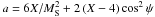 , b = X(X + 5)sin2ψ, c = 3X2(X − 1)sin2ψ. Here it was suggested that the adiabatic index γ = 5/3.
Firstly, let’s estimate the Mach number as MS ≈ vLFC/vS, where vLFC ≈ 2.2 × 108 cm s-1 is the velocity of the LFC source (see Table 1) and vS is the upstream sound speed. Within the standard range of coronal temperatures T ≃ 1−2 MK, we find MS ≈ 10.2−14.5. Now we can find the physically meaningful solution of the quadratic equation and thus estimate the Alfvén-Mach number as MA ≈ 1.06−1.16 within the entire range of ψ ∈ (0,π/2). The upstream magnetic field Bu can be estimated as  G, where nu is the upstream electron plasma density in cm-3, which was already estimated in Sect. 2.5 using the observed frequency range of the type II burst as nu ≈ 5 × 10⁷−1 × 109 cm-3. Thus, we find Bu ≈ 6−33 G and also the plasma parameter
  . These values of Bu are about six times larger than those obtained in Sect. 2.5. It is not surprising, since the used empirical formula of Dulk & McLean (1978) is a generalization of observational data of many different active regions.
A more important inference from the above estimations is the small value of MA ≈ 1.06−1.16. It indicates that the upstream Alfvén speed could be vA ≈ vLFC/MA ≈ 1900−2080 km s-1, which is significantly larger than the observed speeds of the eruptive plasmas (see Table 1). At first glance, this may seemed contradictory to the piston-driven shock wave scenario, which, as it was argued in Sects. 4.1.1 and 4.1.2, is preferable in this event. However, numerical simulations of Pomoell et al. (2008, 2009) have shown that in the inhomogeneous corona even a sub-Alfvénic plasma ejection can launch a shock wave.
It makes sense also to note that the inferred Alfvén-Mach number is less than the critical Alfvén-Mach number Mc ≈ 2.76 for a resistive shock wave (e.g., Treumann 2009). Consequently, the shock wave could be subcritical, regardless of whether it was quasi-parallel or quasi-perpendicular. Electrons were definitely accelerated by the shock wave in the event studied since the type II burst emission was observed. This gives evidence that subcritical shock waves can accelerate electrons in the corona. This fact could be interesting for theories of charged particle acceleration since a supercritical shock wave is generally believed to accelerate charged particles (e.g., Mann 1995; Treumann 2009).
4.2.2. Scenario 2
In principle, Scenario 2 could also be implemented in the studied event. One of the possible cases is schematically illustrated in Fig. 2b of Holman & Pesses (1983). The efficiency of the type II radio emission production in the upstream zone by shock-drift accelerated electrons depends critically on the angle (ψ) between the shock normal at a given point and the upstream magnetic field. Radio emission from the upstream region is then expected only if ψ is restricted to a narrow angular range, within a few degrees of 90°. In the case of a particular mutual arrangement of the shock wave front and the upstream magnetic field, two separate regions of electron acceleration and thus of enhanced radio emission can be expected. No apparent contradictions between the idea of Holman & Pesses (1983, especially illustrated in their Fig. 2b) and our observations are found. If, in the event studied here, the shock wave front was curved rather than plane, the apparent location of the HFC sources below the LFC ones could be mainly due to the projection effect.
Contrary to Scenario 1, Scenario 2 has an important principal drawback: it can not easily explain correlated intensity and frequency drift variations of the LFC and HFC observed in many type II bursts (e.g., Vršnak et al. 2001) as well as in the studied event. It also has difficulties to explain the common range of the relative band split Δf/f ≈ 0.1−0.2 in many type II bursts because the solar corona is very inhomogeneous (e.g., Cairns 2011). In our opinion, these facts make Scenario 2 less favorable than Scenario 1.
4.2.3. An alternative scenario
Cairns (1994) reported observations of fine-structured electromagnetic emissions both from the solar wind and from the Earth’s foreshock. It was shown that for fundamental emission, the fine structures above the local plasma frequency fp corresponded to bands separated by near half harmonics of the electron cyclotron frequency fce, i.e., by nfce/2, where n is a natural number. For harmonic emission, the separation was nfce.
In our case, the frequency separation for the harmonic emission of the observed type II burst is Δf ≈ 0.16fLFC, i.e., Δf ≈ 30−60 MHz. The magnetic field estimated in the previous sections is within the range of B1 ≈ 6−33 G (using the upstream-downstream hypothesis) or B2 ≈ 1−6 G (using the formula of Dulk & McLean 1978). Consequently, the electron cyclotron plasma frequency should be fce1 ≈ 17−92 MHz in the first case and fce2 ≈ 3−17 MHz in the second case. While fce1 is in agreement with the observed separation of the LFC and HFC, fce2 is not. However, the first case corresponds to the situation when the LFC sources were emitted from the upstream region, whereas the HFC sources were emitted from the downstream region. This is in contradiction with Cairns (1994) findings, since he reported that the fine-structured emissions were radiated from the upstream region of the Earth’s bow shock only.
5. Final remarks
In this paper, the detailed analysis of the partially occulted solar eruptive event of 3 November 2010 was presented. Special attention was given to the search of potential links between the dynamics of eruptive magnetoplasma structure well observed at different temperatures with AIA/SDO and the sources of the split-band decimetric/metric type II burst (harmonic emission) observed with the NRH. Simultaneous high-precision observations of eruptive structures and spatially resolved observations of decimetric/metric type II bursts are still rare. This paper deals with the event for which such observations were performed with unprecedented quality. Bain et al. (2012) also investigated for this event the origin of the type II burst, but we have presented here a more detailed discussion and also addressed the nature of the type II band splitting.
The origin of coronal type II bursts is still under debate. It is not clear yet whether it is attributed to blast shock waves or to piston shock waves driven by eruptive magnetoplasma structures such as magnetic flux ropes. It is found that the most preferable agent responsible for the coronal type II burst studied in the paper is the piston shock wave ignited by the eruptive multitemperature plasmas. The most compelling evidence in favor of this conclusion is twofold: the location of the type II burst sources above the apex of the eruptive plasma LE and the same propagation direction of the type II burst sources and erupting plasma apex. Since these coupled observational facts cannot be easily explained by the blast shock wave, we exclude this possibility. It is also found that at the start of the type II burst, its sources were located just above the apex of the eruptive plasma LE and moved with a speed equal to the speed of the eruptive plasma LE. But about 20 s later, the speed of the type II burst sources became twice as fast as that of the eruptive plasma LE. This indicates that initially the shock wave, which could be responsible for the type II burst emission, was of a piston type, but it could later transform to a free propagating blast wave. This observation is in close agreement with the results of numerical simulations made recently by Pomoell et al. (2008, 2009).
Strong observational evidence was found in favor of the hypothesis that the observed type II burst splitting can be explained by radio sources simultaneously produced upstream and downstream of the shock wave front. The LFC source was located in the upstream region, whereas the HFC source was located in the downstream region, below the shock wave front but above the LE of the eruptive plasmas, i.e., in the magnetosheath. This can easily explain the slightly lower location of the HFC source relative to the location of the LFC source observed at the same frequency. Based on the band-splitting effect, we estimated the Alfvén-Mach number as MA ≈ 1.06−1.16, which is less than the critical Alfvén-Mach number. This indicates that in the event studied the shock wave could be subcritical. Nevertheless, due to the fact that the type II burst emission was observed, we came to the conclusion that even subcritical shock waves could accelerate electrons in the lower corona.
All the conclusions presented above were obtained on the basis of only one particular event analysis. Further investigations of similar well observed events are required to investigate whether they are common or not. We emphasize here that high-precision, high-cadence, multiwavelength AIA/SDO observations seem very promising to identify the direct evidence (e.g., jumps of density and/or temperature) of shock waves formation in the lower corona. The first such evidence has already been reported by Kozarev et al. (2011) and Ma et al. (2011). Thus, further analysis of joint AIA/SDO and NRH observations of solar events accompanied by decimetric-metric type II bursts could bring new helpful results on the formation of shock waves in the lower corona and on their physical properties. Such joint observations are most probably rare. In addition, fine-tuned numerical MHD modeling combined with the kinetic simulations of charged particles is highly required.
Acknowledgments
The authors are grateful to A. Klassen, A. Kerdraon, H. Bain, and S. Krucker for helpful discussions, to K. Reeves, who initially provided the AIA/SDO data, and to H. Reid for assistance with the text revision. Courtesy of NASA/SDO and the AIA team. We also thanks to all teams of the instruments (RHESSI, EUVI/SECCHI, GOES, RSTN, Phoenix) whose data are used in the paper. The work was partially supported by the Russian Foundation for Basic Research (project 10-02-01285-a), by the State Contract No. 14.740.11.0086, and by the grant NSch-3200.2010.2. A.C.L.C. acknowledges the award of a Marie Curie International Incoming Fellowship and the hospitality of Paris Observatory. N.V. acknowledges support from the Centre National d’Études Spatiales (CNES) and from the French program on Solar Terrestrial Physics (PNST) of CNRS/INSU. The NRH is funded by the French Ministry of Education, the CNES, and the Région Centre.
References
- Aurass, H. 1997, in Coronal Physics from Radio and Space Observations, ed. G. Trottet, Lecture Notes in Physics (Berlin: Springer Verlag), 483, 135 [Google Scholar]
- Bain, H. M., Krucker, S., Glesener, L., & Lin, R. P. 2012, ApJ, 750, 44 [Google Scholar]
- Bale, S. D., Reiner, M. J., Bougeret, J.-L., et al. 1999, Geophys. Res. Lett., 26, 1573 [NASA ADS] [CrossRef] [Google Scholar]
- Benz, A. O., Battaglia, M., & Vilmer, N. 2011, Sol. Phys., 273, 363 [NASA ADS] [CrossRef] [Google Scholar]
- Brueckner, G. E., Howard, R. A., Koomen, M. J., et al. 1995, Sol. Phys., 162, 357 [NASA ADS] [CrossRef] [Google Scholar]
- Cairns, I. H. 1994, J. Geophys. Res., 99, 23505 [NASA ADS] [CrossRef] [Google Scholar]
- Cairns, I. H. 2011, Coherent Radio Emissions Associated with Star System Shocks, eds. M. P. Miralles, & J. Sánchez Almeida, 267 [Google Scholar]
- Carmichael, H. 1964, NASA Spec. Publ., 50, 451 [Google Scholar]
- Cheng, X., Zhang, J., Liu, Y., & Ding, M. D. 2011, ApJ, 732, L25 [NASA ADS] [CrossRef] [Google Scholar]
- Chian, A. C.-L., & Muñoz, P. R. 2011, ApJ, 733, L34 [NASA ADS] [CrossRef] [Google Scholar]
- Cliver, E. W., Webb, D. F., & Howard, R. A. 1999, Sol. Phys., 187, 89 [NASA ADS] [CrossRef] [Google Scholar]
- Dauphin, C., Vilmer, N., & Krucker, S. 2006, A&A, 455, 339 [NASA ADS] [CrossRef] [EDP Sciences] [Google Scholar]
- Démoulin, P. 2008, Annales Geophysicae, 26, 3113 [CrossRef] [Google Scholar]
- Dulk, G. A. 1970, PASA, 1, 308 [Google Scholar]
- Dulk, G. A., & McLean, D. J. 1978, Sol. Phys., 57, 279 [NASA ADS] [CrossRef] [Google Scholar]
- Foullon, C., Verwichte, E., Nakariakov, V. M., Nykyri, K., & Farrugia, C. J. 2011, ApJ, 729, L8 [NASA ADS] [CrossRef] [Google Scholar]
- Gosling, J. T., Thomsen, M. F., Bame, S. J., & Russell, C. T. 1989, J. Geophys. Res., 941, 10011 [NASA ADS] [CrossRef] [Google Scholar]
- Gosling, J. T., Eriksson, S., McComas, D. J., Phan, T. D., & Skoug, R. M. 2007, J. Geophys. Res. (Space Phys.), 112, A08106 [NASA ADS] [CrossRef] [Google Scholar]
- Hirayama, T. 1974, Sol. Phys., 34, 323 [NASA ADS] [CrossRef] [Google Scholar]
- Hoang, S., Pantellini, F., Harvey, C. C., et al. 1992, in Solar Wind Seven Colloquium, eds. E. Marsch, & R. Schwenn, 465 [Google Scholar]
- Hoang, S., Lacombe, C., MacDowall, R. J., & Thejappa, G. 2007, J. Geophys. Res. (Space Phys.), 112, 9102 [NASA ADS] [CrossRef] [Google Scholar]
- Holman, G. D., & Pesses, M. E. 1983, ApJ, 267, 837 [NASA ADS] [CrossRef] [Google Scholar]
- Huang, S., Deng, X., Zhou, M., et al. 2012, Chin. Sci. Bull., 57, 1455 [CrossRef] [Google Scholar]
- Kerdraon, A., & Delouis, J.-M. 1997, in Coronal Physics from Radio and Space Observations, ed. G. Trottet, Lecture Notes in Physics (Berlin: Springer Verlag), 483, 192 [Google Scholar]
- Khan, J. I., & Aurass, H. 2002, A&A, 383, 1018 [NASA ADS] [CrossRef] [EDP Sciences] [Google Scholar]
- Klassen, A., Aurass, H., Klein, K.-L., Hofmann, A., & Mann, G. 1999, A&A, 343, 287 [NASA ADS] [Google Scholar]
- Klassen, A., Pohjolainen, S., & Klein, K.-L. 2003, Sol. Phys., 218, 197 [NASA ADS] [CrossRef] [Google Scholar]
- Klein, K.-L., Khan, J. I., Vilmer, N., Delouis, J.-M., & Aurass, H. 1999, A&A, 346, L53 [NASA ADS] [Google Scholar]
- Knock, S. A., & Cairns, I. H. 2005, J. Geophys. Res. (Space Phys.), 110, A01101 [Google Scholar]
- Kopp, R. A., & Pneuman, G. W. 1976, Sol. Phys., 50, 85 [NASA ADS] [CrossRef] [Google Scholar]
- Kozarev, K. A., Korreck, K. E., Lobzin, V. V., Weber, M. A., & Schwadron, N. A. 2011, ApJ, 733, L25 [NASA ADS] [CrossRef] [Google Scholar]
- Krueger, A. 1979, Introduction to solar radio astronomy and radio physics (Dordrecht: Reidel) [Google Scholar]
- Lee, J. S. 1980, IEEE Transactions on Pattern Analysis and Machine Intelligence, Vol. PAMI-2, No. 2, 165 [Google Scholar]
- Lemen, J. R., Title, A. M., Akin, D. J., et al. 2012, Sol. Phys., 275, 17 [NASA ADS] [CrossRef] [Google Scholar]
- Lengyel-Frey, D. 1992, J. Geophys. Res., 97, 1609 [Google Scholar]
- Lowe, R. E., & Burgess, D. 2000, Geophys. Res. Lett., 27, 3249 [NASA ADS] [CrossRef] [Google Scholar]
- Ma, S., Raymond, J. C., Golub, L., et al. 2011, ApJ, 738, 160 [CrossRef] [Google Scholar]
- Mann, G. 1995, in Coronal Magnetic Energy Releases, eds. A. O. Benz, & A. Krüger, Lecture Notes in Physics (Berlin: Springer Verlag), 444, 183 [Google Scholar]
- McLean, D. J. 1967, PASA, 1, 47 [Google Scholar]
- Moullard, O., Burgess, D., Salem, C., et al. 2001, J. Geophys. Res., 106, 8301 [NASA ADS] [CrossRef] [Google Scholar]
- Nelson, G. J., & Melrose, D. B. 1985, Type II bursts, eds. D. J. McLean, & N. R. Labrum, 333 [Google Scholar]
- Nelson, G. J., & Robinson, R. D. 1975, PASA, 2, 370 [NASA ADS] [CrossRef] [Google Scholar]
- O’Dwyer, B., Del Zanna, G., Mason, H. E., Weber, M. A., & Tripathi, D. 2010, A&A, 521, A21 [NASA ADS] [CrossRef] [EDP Sciences] [Google Scholar]
- Pohjolainen, S., Pomoell, J., & Vainio, R. 2008, A&A, 490, 357 [NASA ADS] [CrossRef] [EDP Sciences] [Google Scholar]
- Pomoell, J., Vainio, R., & Kissmann, R. 2008, Sol. Phys., 253, 249 [NASA ADS] [CrossRef] [Google Scholar]
- Pomoell, J., Vainio, R., & Pohjolainen, S. 2009, in IAU Symp. 257, eds. N. Gopalswamy, & D. F. Webb, 493 [Google Scholar]
- Priest, E. R. 1982, Solar magneto-hydrodynamics (Dordrecht, Holland, Boston: D. Reidel Co.), 74 [Google Scholar]
- Pulupa, M., & Bale, S. D. 2008, ApJ, 676, 1330 [NASA ADS] [CrossRef] [Google Scholar]
- Reeves, K. K., & Golub, L. 2011, ApJ, 727, L52 [NASA ADS] [CrossRef] [Google Scholar]
- Reiner, M. J., Kaiser, M. L., Fainberg, J., & Stone, R. G. 1998, J. Geophys. Res., 1032, 29651 [Google Scholar]
- Scherrer, P. H., Schou, J., Bush, R. I., et al. 2011, Sol. Phys., 365 [Google Scholar]
- Schmidt, J. M., & Cargill, P. J. 2003, J. Geophys. Res. (Space Phys.), 108, 1023 [NASA ADS] [CrossRef] [Google Scholar]
- Smerd, S. F., Sheridan, K. V., & Stewart, R. T. 1974, in Coronal Disturbances, ed. G. A. Newkirk, IAU Symp., 57, 389 [Google Scholar]
- Smerd, S. F., Sheridan, K. V., & Stewart, R. T. 1975, ApL, 16, 23 [Google Scholar]
- Sturrock, P. A. 1966, Nature, 211, 695 [NASA ADS] [CrossRef] [Google Scholar]
- Thejappa, G., & MacDowall, R. J. 2000, ApJ, 544, L163 [NASA ADS] [CrossRef] [Google Scholar]
- Treumann, R. A. 2009, A&ARv, 17, 409 [NASA ADS] [Google Scholar]
- Treumann, R. A., & Labelle, J. 1992, ApJ, 399, L167 [NASA ADS] [CrossRef] [Google Scholar]
- Vandas, M., & Karlický, M. 2000, Sol. Phys., 197, 85 [NASA ADS] [CrossRef] [Google Scholar]
- Vourlidas, A., & Ontiveros, V. 2009, in AIP Conf. Ser. 1183, eds. X. Ao, & G. Z. R. Burrows, 139 [Google Scholar]
- Vršnak, B., & Cliver, E. W. 2008, Sol. Phys., 253, 215 [NASA ADS] [CrossRef] [Google Scholar]
- Vrsnak, B., & Lulic, S. 2000, Hvar Observatory Bull., 24, 17 [Google Scholar]
- Vršnak, B., Aurass, H., Magdalenić, J., & Gopalswamy, N. 2001, A&A, 377, 321 [Google Scholar]
- Vršnak, B., Magdalenić, J., Aurass, H., & Mann, G. 2002, A&A, 396, 673 [NASA ADS] [CrossRef] [EDP Sciences] [Google Scholar]
- Vršnak, B., Warmuth, A., Temmer, M., et al. 2006, A&A, 448, 739 [Google Scholar]
- Wang, Y., Wei, F. S., Feng, X. S., et al. 2010, Phys. Rev. Lett., 105, 195007 [NASA ADS] [CrossRef] [Google Scholar]
- Wei, F., Liu, R., Fan, Q., & Feng, X. 2003, J. Geophys. Res. (Space Phys.), 108, 1263 [Google Scholar]
- Wild, J. P., & Smerd, S. F. 1972, ARA&A, 10, 159 [NASA ADS] [CrossRef] [Google Scholar]
- Wuelser, J.-P., Lemen, J. R., Tarbell, T. D., et al. 2004, in SPIE Conf. Ser. 5171, eds. S. Fineschi, & M. A. Gummin, 111 [Google Scholar]
- Zheleznyakov, V. V. 1970, Radio emission of the sun and planets (Oxford: Pergamon Press) [Google Scholar]
All Tables
Velocity estimations of different moving objects observed in course of the 3 November 2010 eruptive event.
All Figures
|
Fig. 1 Dynamic radio spectrograms and lightcurves of radio, soft, and hard X-ray emissions during the 3 November 2010 eruptive event. Solar radio flux density measured by the telescope in San Vito (RSTN) at 245 MHz is divided by a factor of ten for clarity. The vertical dashed line indicates the peak time (12:14:00 UT) of the hard X-ray and microwave bursts. |
| In the text | |
|
Fig. 2 Active area near the eastern limb of the Sun in the impulsive phase of the 3 November 2010 eruptive flare. AIA 211 Å a) and 131 Å b) base-difference images are overlaid by the RHESSI 6−12 keV (12:13:54−12:14:14 UT; light green) and 25−50 keV (12:13:54–12:14:14 UT; red) contours (20%, 40%, 60%, 80% of the peak flux), indicating locations of the flare soft and hard X-ray sources, respectively. AIA 211 Å base image was made at ≈12:00:02 UT and 131 Å base image – at ≈12:00:11 UT. Yellow ellipses are the NRH 445 MHz contours (70%, 80%, and 90% of the peak flux), which indicate the location of the decimetric radio emission source at the same moment. The thick dashed yellow straight line indicates a projection of the radius-vector passing through the centroid of the flare soft X-ray source onto the image plane. |
| In the text | |
|
Fig. 3 Base-difference image of the active area near the eastern limb of the Sun made by AIA in 193 Å channel at ≈12:15:08 UT. The AIA base image was made at ≈12:00:08 UT. Dashed parabolic lines of different colors indicate the fitted LE of the eruptive plasma at an appropriate moment (see colorbar). The found parabolas’ apices are marked by squares. Green dashed straight line indicates a projection of the radius-vector passing through the flare onto the image plane (as in Fig. 2). |
| In the text | |
|
Fig. 4 Background-subtracted dynamic radio spectrum of the 3 November 2010 solar eruptive event obtained with the Phoenix-4 spectrograph (upper panel). Green and turquoise horizontal strokes with diamonds in the middle indicate respectively when the sources of the LFC and HFC of the type II burst’s H-component (H) were observed by the NRH for the first 10 s after its first appearance. Crosses of the same colors represent the LFC’s and HFC’s first appearence at different frequencies below 180 MHz according to the San Vito spectrograph data. Dark blue horizontal strokes with diamonds indicate the 10 s intervals of the HFC maximal intensity in appropriate frequencies. Time profiles of radio flux density measured by the NRH from the south-eastern sector of the Sun with time cadence of 1 s as well as one second solar radio flux density measured by San Vito telescope (RSTN) at 610 MHz are shown by the black and white curves, respectively. Four seconds RHESSI corrected count rates at the 6−12 and 25−50 keV ranges are depicted by the blue and red curves, respectively. The green vertical dashed line indicates the start time of the type II burst’s H-component. Black vertical dash-dotted lines marked by (a), (b), (c), (d) letters on top of the panel indicate four different moments for which four panels of Fig. 7 were made. The orange dash-dotted line connects the separated fragments of the type II burst’s F-component (F). The thin turquoise rectangular box indicates a piece of the spectrogram, which is represented in the lower panel using a slightly different color palette. The band splitting of the type II burst H-component is clearly seen. |
| In the text | |
|
Fig. 5 Average positions of the type II burst’s LFC and HFC sources observed by NRH at several frequencies during the 3 November 2010 eruptive event. Error bars of the LFC and HFC source centroid estimations are shown. Positions of the double coronal hard X-ray source observed by RHESSI in the flare impulsive phase are also plotted by two black asterisks for comparison. The straight black dashed line indicates a projection of the radius-vector passing through the double coronal HXR source onto the image plane. The solar optical limb is represented by black solid arc-like line. |
| In the text | |
|
Fig. 6 Partial time sequence of AIA/SDO 131, 211, and 193 Å base-difference images in between 12:13:10 UT and 12:16:30 UT of 3 November 2010. Overplotted are the iso-intensity contours (50%, 60%, 70%, 80%, and 90% of the maximum) of the LFC source observed by NRH at different frequencies at a vicinity of times of its first appearance (indicated in the upper left corner of the AIA 131 Å images). One-second integrated NRH data is used. The closest AIA images in time to the NRH ones are shown (the time difference is less than eight seconds in each case). Solar limb is depicted by the thick white line. The red dashed straight line in all panels indicates a projection of the radius vector passing through the X-ray flare onto the image plane. The AIA’s field of view is less than that of the NRH. |
| In the text | |
|
Fig. 7 Composite base-difference images of the active area near the eastern limb of the Sun made by AIA in 131 Å (turquoise) and 211 Å (purple) passbands at four different times of the 3 November 2010 event. These times are marked by dash-dotted vertical lines in Figs. 4 and 8. Green, yellow, and red dashed parabolas on panels a), b) and c), respectively, indicate the approximated LE of eruptive plasma observed by AIA in 211 Å passband. The parabolas’ colors are consistent with the colorbar in Fig. 3. Solid lines of different colors are the NRH contours (95% of the peak flux), which indicate locations of centroids of the type II burst sources at different frequencies (indicated within each panel) at appropriate moments. All AIA and NRH images are matched within 5 s. Red dashed line in all panels indicates a projection of the radius-vector passing through the X-ray flare onto the image plane. |
| In the text | |
|
Fig. 8 Height-time plot of the type II burst sources observed by NRH versus different parts of the multi-temperature eruptive plasmas observed with AIA/SDO. The double coronal hard X-ray source heights observed by RHESSI in the flare impulsive phase are also plotted by orange crosses with diamonds. Black dashed and dash-dotted vertical lines indicate the beginning of the type II burst and four time moments for which panels a)–d) of Fig. 7 were created, respectively. Error bars of all object estimations are shown with vertical and horizontal strokes of appropriate colors. Heights of the type II burst’s LFC and HFC sources are given for those time intervals, which are shown by the same colors (green, turquoise, and dark blue) in Fig. 4. The least square fittings of the observational data points with the linear functions are plotted by the straight lines of appropriate colors. |
| In the text | |
|
Fig. 9 Schematic illustration of the 3 November 2010 eruptive event observations combined with their interpretation in the frame of the upstream-downstream scenario (see text). View is from the heliographic north pole. Direction to the Earth is marked by a thick black arrow. Notations: (1) hypothetical shock wave, (2) LFC source of the type II burst, (3) its HFC source, (4) turbulent magnetosheath, (5) warm (T ≈ 1−2 MK) plasma rim and (6) its LE, (7) hot (T ≃ 10 MK) erupting flux rope or plasma blob if observed from the Earth, (8) photosphere. Thin black arrows show directions of the eruptive plasmas, shock wave, LFC and HFC sources motion. Lengths of the arrows are proportional to the corresponding velocities of motion. Levels of constant undisturbed background electron plasma concentration, assuming the natural gravitational stratification, are marked by black dashed arc-lines, and n1 > n2 > n3. |
| In the text | |
|
Fig. 10 Schematic illustration of the lower location of the HFC sources of the type II burst with respect to the LFC sources observed at the same frequency. Panel a) corresponds to an instant t1, which is before the instant t2 (t2 > t1) of panel b). Solar surface is depicted by thick black line with inclined ticks on the right. Thick dashed arc-like line shows the shock wave front. Light and dark grey ellipses represent the LFC and HFC sources, respectively. Horizontal arrow shows the direction of their movement. Levels of constant plasma density are shown by vertical straight dashed and dotted lines. Corresponding plasma densities are marked by n1, |
| In the text | |
Current usage metrics show cumulative count of Article Views (full-text article views including HTML views, PDF and ePub downloads, according to the available data) and Abstracts Views on Vision4Press platform.
Data correspond to usage on the plateform after 2015. The current usage metrics is available 48-96 hours after online publication and is updated daily on week days.
Initial download of the metrics may take a while.