| Issue |
A&A
Volume 547, November 2012
|
|
|---|---|---|
| Article Number | A73 | |
| Number of page(s) | 8 | |
| Section | The Sun | |
| DOI | https://doi.org/10.1051/0004-6361/201118608 | |
| Published online | 31 October 2012 | |
Solar flare hard X-ray spikes observed by RHESSI: a statistical study
1 School of Astronomy & Space Science, Nanjing University, 210093 Nanjing, PR China
e-mail: This email address is being protected from spambots. You need JavaScript enabled to view it.
2 Shanghai Astronomical Observatory, Chinese Academy of Sciences, 200030 Shanghai, PR China
3 Department of Physics, Montana State University, Bozeman MT 59717-3840, USA
4 Key Laboratory of Modern Astronomy and Astrophysics (Ministry of Education), Nanjing University, 210093 Nanjing, PR China
5 New Jersey Institute of Technology, 323 Martin Luther Kind Blvd., Newark, NJ 07102, USA
Received: 8 December 2011
Accepted: 14 September 2012
Abstract
Context. Hard X-ray (HXR) spikes refer to fine time structures on timescales of seconds to milliseconds in high-energy HXR emission profiles during solar flare eruptions.
Aims. We present a preliminary statistical investigation of temporal and spectral properties of HXR spikes.
Methods. Using a three-sigma spike selection rule, we detected 184 spikes in 94 out of 322 flares with significant counts at given photon energies, which were detected from demodulated HXR light curves obtained by the Reuven Ramaty High Energy Solar Spectroscopic Imager (RHESSI). About one fifth of these spikes are also detected at photon energies higher than 100 keV.
Results. The statistical properties of the spikes are as follows. (1) HXR spikes are produced in both impulsive flares and long-duration flares with nearly the same occurrence rates. Ninety percent of the spikes occur during the rise phase of the flares, and about 70% occur around the peak times of the flares. (2) The time durations of the spikes vary from 0.2 to 2 s, with the mean being 1.0 s, which is not dependent on photon energies. The spikes exhibit symmetric time profiles with no significant difference between rise and decay times. (3) Among the most energetic spikes, nearly all of them have harder count spectra than their underlying slow-varying components. There is also a weak indication that spikes exhibiting time lags in high-energy emissions tend to have harder spectra than spikes with time lags in low-energy emissions.
Key words: Sun: flares / Sun: X-rays, gamma rays
© ESO, 2012
1. Introduction
Solar flare emission at sub-second timescales was reported in hard X-ray (HXR) observations by satellite-borne HXR spectrometers in the 70 s and 80 s (van Beek et al. 1974, 1976; Hoyng et al. 1976; de Jager & de Jonger 1978; Kiplinger et al. 1983, 1984, 1989). Examining HXR flares observed by the Solar Maximum Mission (SMM) with time resolutions of 128 ms and 10 ms, Kiplinger et al. (1983) found that 53 out of nearly 3000 flares produce several hundred fast spikes with durations as short as 45 ms. These energetic flare bursts on short timescales are believed to be nonthermal in nature, and their temporal and spectral properties place constraints on the physical nature of the source.
Several physical mechanisms are proposed to produce HXR spikes as rapid and short-lasting enhancement over the slow-varying underlying emission. Magnetic reconnection is believed to provide the means of converting energy stored in the magnetic fields into thermal and kinetic energies (e.g., Carmichael 1964; Sturrock 1966; Hirayama 1974; Kopp & Pneuman 1976; Priest & Forbes 2000; Aschwanden 2004). Particles may be accelerated to high energies at the reconnection site in the corona and then deposited at the chromosphere emitting HXR radiation by bremsstrahlung. It is known that along the length of the pre-connection current sheet, a tearing mode instability may occur to trigger reconnection and form magnetic islands (Furth et al. 1963; Sturrock 1966). Formation of the magnetic islands by tearing instability and subsequent interactions between these magnetic islands, namely the dynamic magnetic reconnection (Kliem et al. 2000, and references therein), are considered to account for fast variations in nonthermal emissions (Aschwanden 2002, and references therein). Kaufmann (1996) also proposed that in the magnetically complex solar active regions, one would expect to have multiple, primeval explosive compact synchrotron sources flashing at different times, building up what is usually described as the onset of the impulsive phase of the bursts. Different spikes may indeed originate at various sites, as suggested by one mm-wave observation (Correia et al. 1995). The primeval compact sources might originate from a number of plasma instabilities, such as in twisted magnetic fields, and magnetic flux networks (Sturrock & Uchida 1981; Sturrock et al. 1984). Another proposed mechanism to produce fine structures in HXR and microwaves concerns nonthermal electron injections. Electron beams become unstable when fast particles of a nonthermal electron distribution outpace the slower ones from the thermal or suprathermal tail during their propagation along magnetic fields lines. These unstable electron beams cause discrete electron injections and finally contribute to spiky HXR emissions.
The kinematics of energized electrons and the energy dependence of their collisional interactions in high-density plasmas in solar flares can be probed by accurate time delay measurements between HXR emission at different energies. There is a variety of the time delay mechanisms operating in solar flares that can be used as a diagnostics of physical parameters. In the thick-target model (Brwon 1971; Fisher et al. 1985; Emslie & Nagai 1985; MacNeice et al. 1984; Mariska et al. 1989) for HXR emission in solar flares, electron acceleration is assumed to occur in flaring loops at coronal heights, while HXR bremsstrahlung emission is produced in the chromosphere. Under this assumption, the velocity spectrum of the accelerated electrons causes time-of-flight differences that are expected to result in a delay of the lower energy HXR emission with respect to that in higher energies (Aschwanden et al. 1995; Brown et al. 1998). A different case is that the HXR emission in higher energies lags behind the emission in lower energies (Aschwanden et al. 1997; Qiu et al. 2004). Two basic models have been proposed for the latter: the trap-plus-precipitation model (Melrose & Brown 1976; Vilmer et al. 1982; Bespalov et al. 1987) and the second-step acceleration model (Bai & Ramaty 1979). In the trap model, the lag of the high-energy emission occurs because the collisional timescale increases with the particle energy. This delays the escape from the trap and the subsequent precipitation and, thus, the resulting thick-target HXR emission. In the second-step acceleration model, a second-stage process is invoked to accelerate super-thermal electrons to higher energies. Both of these models produce an energy delay with a sign opposite to that caused by the time-of-flight effect. In particular, whether the low-energy emission lags or the high-energy emission lags depends on the relative importance of these two mechanisms. Involved in different mechanisms during the flare eruptions, we study the meaningful energy-dependent time delay that occurs in the spikes with high temporal and spectral resolving observations.
The Reuven Ramaty High Energy Solar Spectroscopic Imager (RHESSI, Lin et al. 2002) has observed several tens of thousands of flares with unprecedented temporal and spectral resolution since its launch in early 2002. It uses a set of nine rotating modulation collimators, each consisting of a high spectral resolution germanium detector. As the spacecraft rotates, the grids transmit a rapidly time-modulated fraction of the incident flux. To identify fine time structures in flare HXR emissions observed by RHESSI, a demodulation algorithm was recently developed to remove the modulation pattern from the HXR light curves. The demodulation code was applied to some flares that were found to produce fast-varying spikes evident in HXR emissions of over 100 keV (Qiu et al. 2012, hereafter, Paper I). Ten spikes analyzed in Paper I exhibit a sharp rise and decay with a duration of less than 1 s, with the designated instrument resolution of 125 ms. Energy-dependent time lags are found in some spikes, which are consistent with the time-of-flight of precipitating electrons estimated from imaging observations. All these spikes show a harder spectrum than the underlying components, indicating that the spectral properties are closely related to timescales.
These ten spikes analyzed in Paper I are produced in a few randomly selected flares. It is important to conduct a systematic search for fast spikes using existing databases. In the present study, we examine all flares observed by RHESSI in 2002, and apply the demodulation code to flares with more than 100 data counts in 12 − 25 keV to identify HXR spikes in a few photon energy bands. We then conduct a statistical study of spike-productive flares and the temporal and spectral properties of HXR spikes. The paper is organized as follows. Observations and data analysis are given in Sect. 2. Properties of HXR spikes are presented in Sect. 3, followed by discussions and conclusions in Sect. 4.
2. Observations and data analysis
2.1. Selection of HXR spikes
Using the demodulation algorithm as described in Paper I, we examined several RHESSI observations of flare bursts for HXR spikes, and analyzed their temporal and spectral properties. Our database includes all RHESSI HXR flares in the year 2002. According to the RHESSI flare list, 5302 flares were observed in 2002. Among them, we selected relatively strong events with peak count rates in 12 − 25 keV greater than 100 counts s-1 and significant emission in the photon energy range greater than 50 keV. This information was directly acquired from the RHESSI flare list. Only 322 flares satisfied these two pre-analysis selection criteria and were analyzed with the demodulation code. These are our final sample for the statistical study.
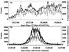 |
Fig. 1 Demodulated RHESSI HXR light curves (dark) in comparison with summed raw data counts (gray). The light curves are acquired at 25 − 100 keV. The demodulated light curves correspond to the count rate y-axis and the summed raw data are related to the count y-axis. The top panel shows an event on 2002 March 17 that exhibits fast-varying spikes. The bottom panel shows an event on 2002 February 20 without significant fast-varying spikes. The scales of the raw and demodulated light curves are indicated in the left and right y-axis, respectively. |
We applied the demodulation algorithm to obtain high temporal resolution light curves with a designated cadence of 125 ms. Figure 1 shows examples of high-candence flare HXR light curves at 25−100 keV that are demodulated from the raw data. A large number of fluctuations are present in the raw data set, most of which, however, were removed in the demodulated light curves. Clearly, not all flares produce sufficiently significant HXR spikes to be picked out by the selection rule. Figure 1a shows an event with evident fast-varying structures, the spike at 19:27:43 UT, while for the event in Fig. 1b no outstanding fast varying spikes can be recognized in the demodulated light curves. One cannot tell whether a flare produces fast-varying spikes from undemodulated raw data.
To identify spikes, we subtracted from demodulated light curves I(t) a slow-varying component Islow(t), which is obtained by box smoothing I(t) over a smoothing window wsmt. wsmt is taken to be between 4 and 8 s, or 32 to 64 bins. We then obtained the residual intensity as Ir(t) = I(t) − Islow(t). We defined a spike when the residual intensity, Ir(t), in the 25−100 keV band was ≥ nsigσ for three consecutive time bins, where σ is the standard deviation of the residual intensity profile, and nsig = 3,4,5. We used two ways to derive σ. First, we derived a fixed value of σ independent of flare evolution, namely, σ ≡ σ0, where σ0 is the standard deviation of Ir(t) for the entire duration of the flare, which is usually 2−3 min in our data (Fig. 2a). Second, to minimize the effect of statistical noises associated with instantaneous photon counts received by the detector during the evolution of the flare, we also used a time-dependent σ(t) derived in a running box wsig (Figs. 2b, c). Derivation of Islow(t), Ir(t) and σ and selection of HXR spikes by these algorithms is illustrated in Fig. 2 using the event on 2002 August 3 as an example. The left panels in the figure show the demodulated light curve at 25 − 100 keV, superposed with the slow component Islow derived with the three methods. The residuals Ir and σ levels (smooth line) are also plotted at the bottom of each panel. The right panels illustrate the times (x-axis) and energy bands (y-axis: see figure caption) whose residuals exceeded 3σ level. Evidently, the different choices of σ by different combinations of wsmt and wsig result in different populations of spike-productive flares, which will be discussed below. We remark that the selection rules likely give a conservative lower limit of the spike population because of the requirement of three consecutive time bins.
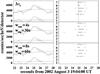 |
Fig. 2 Spike detection algorithm using the three methods (see text) for the event on 2002 August 3. Left panels show the demodulated light curves at 25−100 keV, the slow-varying component (smooth) determined by the three methods, and the residuals (bottom of each panel). The smoothed lines (bottom of each panel) show the sigma levels using the three methods. Right panels show the times (x-axis) and energies (y-axis) of significant residuals recognized by the algorithms. The numbers 1 to 7 along the y-axis indicate energy bands of 10−15, 15−25, 25−40, 40−60, 60−100, 100−300, and 25−100 keV, respectively. The vertical line indicates the most pronounced spikes of the diagrams. |
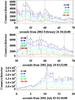 |
Fig. 3 Demodulated RHESSI HXR light curves at varying energies for three flares. The vertical lines indicate the spike times. The y-axis gives the units of the 25 − 100 keV light curves, and light curves at other energies are scaled arbitrarily. |
We applied the selection rules to the 322 samples. Table 1 gives the number of spikes and the number of spike-productive flares using different combinations of wsmt and wsig, including the fixed σ0 criterion, and with nsig = 3. Depending on how σ is defined, the selection rule of 3σ and three consecutive time bins yields 40 to 90 spike-produtive flares, each producing one or two spikes, out of the total of over 5302 flares observed by RHESSI in 2002. This productivity is in general comparable with the result by Kiplinger et al. (1983), who, also by applying the 3σ and consecutive bin criterion, detected 53 spike-productive flares out of 3000 flares observed by SMM. That is to say, fast-varying spikes are detected in 10 − 20% of flares, though observed by different instruments with different methods.
Spike/flare number variations with σ defined by different combinations of wsmt and wsig and with nsig = 3.
Figure 3 shows the demodulated light curves of three flares at varying energies from 25 to 300 keV during the flare eruptions. The designated time bin is 0.125 s. These events all exhibit fast-varying structures on timescale of 1 s or less at most of the energy bins above 25 keV. Signals up to 100 keV are significant and are likely real features. Some of these spikes are also visible in 100−300 keV, though less significant because of reduced counts level.
Using the fixed 3σ0 yields 184 spikes in 94 flares. At 5σ0, there are 54 spikes in 40 flares. At face value, these numbers are significantly greater than the number of spikes that could be produced by statistical noises if the noise distribution followed a simple Poisson (Fig. 4). In reality, the noise distribution is poorly defined, and the noise dependence on instantaneous photon counts is likely much stronger than a Poisson. Therefore, we performed a negative test to identify “negative” spikes by setting nsig = −3, −4, −5 and using the same rule of three consecutive bins. The results of the negative test for a few representative selections are listed in Table 2. Evidently, the negative occurrence is nearly one half of the positive occurrence for the fixed σ0. Even though one cannot ascribe the negative occurrence entirely to the statistical negative because of the way the residual signals are produced, it is conservative to say that about one half of the positive occurrence probably reflects real spike signals.
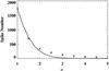 |
Fig. 4 Number of detected spikes varies as σ level increases. The asterisks and the line represent observational and Poisson distributions, respectively. |
When the time-varying σ is employed, understandably, the number of spikes steadily decreases with a smaller wsig or wsmt (Table 1). Table 2 clearly shows that the negative occurrence with the time-varying σ drops to only 10−20% of the positive occurrence. Therefore, most spikes picked out with the time-varying σ approach may be considered as real spikes free from statistical noises. We also note that 2/3 of the spike population via the time-varying σ approach are included in the population from the fixed 3σ0 selection rule.
Spike/flare number variations with different nsig.
The selection with the time-varying σ does not only change the total number of spikes but would, probably, change the distribution of these spikes during the evolution of the flare. For example, the fixed σ0 regardless of the evolution of the flare would misrepresent the noises at different evolution stages. σ0 tends to be smaller than the real standard deviation determined by statistical counts during the flare maximum but larger than the standard deviation during the rise-and-decay phases of the flare when the counts are lower than at the peak. Therefore, the constant σ0 rule might include noisy signals at the peak of the flare, while overlooking real signals during the rise-and-decay phase. On the other hand, by using the time-varying σ, the sample is partly biased against high counts, or the peak phase of the flare.
Because we do not know the true noise distribution, we examined and compared properties of spikes and associated flares selected with the following different rules: fixed σ0, time-varying σ with wsmt = 8 s and wsig = 60 s, and time-varying σ with wsmt = 4 s and wsig = 30 s. The spikes were selected with nsig = 3. Specifically, we illustrated the distribution of the events with respect to the flare magnitude, flare duration, and spike occurrence time, and examine statistical properties of the spikes in terms of their evolution and energetics.
2.2. Event distribution
We compared spike-productive flares with flares that do not produce fast-varying spikes to examine whether they are statistically different populations in terms of flare magnitude and duration. Figure 5 shows the peak count rate distributions of all 322 flares in the sample with a peak count rate exceeding 100, and the spike-associated flares from four different selection rules: 5σ0, 3σ0, 3σ at wsmt = 8 s and wsig = 60 s, and 3σ at wsmt = 4 s and wsig = 30 s. Figure 5 shows that the distribution for the entire sample of 322 flares is steeper than that for the spike-associated flares, suggesting that more intensive flares have in general a greater chance to produce spikes. There is no notable difference in the distributions of the four spike-productive flare populations, suggesting that the majority of selected spikes are not dominated by noise that grows with photon counts.
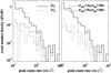 |
Fig. 5 Peak count rate distributions at various criteria denoted in the figure. The upper thick solid line indicates our 322-flare sample. The profile is obviously steeper than all other profiles. |
We also examined whether impulsive flares, compared with gradual events, are more productive in fast-varying spikes. Figure 6 displays the rise time distributions for spike-productive flares in comparison with that of all 322 flares. Here we define the flare rise time as the time difference between the flare peak time and the start time, both referring to emission in 12 − 25 keV provided by the RHESSI flare list. No evident difference is found between these distributions, suggesting that HXR spikes can occur in both impulsive and gradual events.
For the spike-productive flares, we also studied at which time the spikes occur with respect to the evolution stage of the flare bursts. For convenience, we defined a normalized spike occurrence time τspk, which refers to the time difference between the spike peak time and the flare start time normalized to the flare rise time. Therefore, if τspk < 1, the studied spike should occur in the rise phase of the flare; if τspk > 1, the spike occurs during the decay phase. Figure 7 illustrates the occurrence time distributions for the spike populations from varying selection rules. For all populations, nearly all spikes occur before or during the peak of the flare. Clearly, the fixed σ0 selection yields a large percentage, up to 70%, of spikes around the peak times (τspk = 0.8−1.2) of the associated flares. With ever smaller wsig and wsmt, the fraction of spikes during the flare peak is reduced as the σ around the flare peak time increases, while there are more spikes detected during the low-count rise phase. At this stage of research, as the noises of the demodulated flare light curves are not well understood and cannot be independently determined, we did not readily give a preference to a certain selection rule. Therefore, all these spike populations from different selection rules are analyzed in the following study.
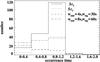 |
Fig. 7 Occurrence time τspk distribution at various criteria as denoted in the figure. See Sect. 2.2 for details. |
Fast-varying spikes were first selected using integrated counts in 25−100 keV. We then demodulated the light curves of these events in photon energy ranges of 25−40, 40−60, 60−100, and 100−300 keV, and searched for the highest energy in which spikes are detected. We denote this energy band by ϵhi. Figure 8 displays the spike distribution with respect to ϵhi. The majority of spikes discovered in 25 − 100 keV can still be seen in 40−60 and 60−100 keV. Indeed, for each population, the peak of the distribution is at 60−100 keV. Nearly 20% of spikes can be detected as high as 100−300 keV. This result suggests that fast-varying spikes are most probably nonthermal in nature.
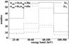 |
Fig. 8 ϵhi distribution at various criteria. See Sect. 2.2 for details. |
All these statistical results indicate that fast-varying spikes are small-scale energetic events produced during the most energetic stage of flares. In particular, they tend to occur during the rise phase of intensive flares. On the other hand, impulsive and gradual flares have an equal chance to produce fast-varying spikes.
In different phases of flare eruption, energy release, and energy transport, the relevant physical processes are quite different. Theoretically, energy release occurs preferentially during the flare rise phase. This seems to support the result of different productivities of spikes in different flare phases.
3. Properties of HXR spikes
HXR spikes at shortest timescales are believed to reflect single energy release events, such as by magnetic reconnection and particle acceleration. We examined the energy-dependent temporal properties of these HXR spikes to gain insight into the nature of the energy release. For the detected spikes, we estimated the spike duration, rise and decay times, the count spectral index, and the energy-dependent time delays and compared them with large flares and previous studies.
To obtain a statistical result of the temporal and spectral properties of HXR spikes, we applied a simplified analysis to all spikes. A more rigorous analysis was also conducted on a dozen prominent spikes out of the selected samples (Paper I), which yields results consistent with the statistical results in the present paper.
3.1. Duration, rise, and decay times
The energy-dependent duration of a spike, τ(ϵ), is estimated to be the time difference between the e-slope start and end times of the spike. We determined the rise and decay times when the spike net intensity, i.e., the intensity with the interpolated underlying component subtracted, drops to e-1 of the peak intensity in both the rise and decay phases. As displayed in Fig. 9, τ(ϵ) ranges from 0.25 to 2.0 s, or 2 to 16 time bins, with an average being 0.98 ± 0.47 s in 25−100 keV for all HXR spikes. The same analysis was applied to light curves in different energy bands, resulting in a mean duration of 1.08 ± 0.39 s, without significant difference in different energies. Therefore, our studies show that the spike duration is nearly independent of photon energies.
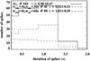 |
Fig. 9 Duration τ(ϵ) distributions at various criteria. The average duration is about 0.9−1.0 s in 25−100 keV. See Sect. 3.1 for details. |
HXR spikes appear to have quite a symmetric sharp rise and decay. The mean e-slope rise time of all spikes is 0.52 ± 0.26 s, and the mean decay time is 0.50 ± 0.25 s. The result indicates no significant difference between the rise and decay times. This is somewhat different from the general scenario of flares, i.e., HXR emission rapidly increases in the impulsive phase, and then decreases relatively gradually in the decay phase.
3.2. Spectral index
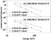 |
Fig. 10 In each panel, the symbols and solid lines show examples of HXR count spectra of integrated spike flux during the spike time in comparison with the count rates spectra of underlying components. Solid lines show the least-squares fit of the spectra to a power-law distribution, and the exponents and their uncertainties from the fit are noted in the figures. The y-axis gives the units of the spike intensities, and the intensities of the underlying component are divided by a number for the clarity of display. S1 is the example we discussed in Fig. 2. |
To study the spike energetics, we fit the spike count spectrum at ≥ 15 keV to a power-law distribution  s ϵ−Γ to obtain the power-law index Γ, as indicated by the straight lines in Fig. 10. Only data in photon energies greater than 15 keV were used to avoid the contamination of thermal bremsstrahlung in lower energies. Among these spikes, reliable least-squares fitting results can be made for only a fraction of spikes. The spectral fitting was applied to the net spike counts integrated over its duration. The net counts of the spike were derived by subtracting the underlying component, which is a mean between the pre-spike and post-spike counts, also integrated over the duration of the spike. As a comparison, we also fit the count spectrum of the underlying component. Figure 10 gives two examples of integrated spike flux with respect to photon energy, i.e., the spike counts spectrum. Also plotted are the directly measured count rate spectra of the underlying components adjacent to the spikes. Figure 10 shows the comparison of spectral indices between the spikes and underlying components. Note that Γ is the index of uncalibrated count spectrum, which is somewhat different from the index of HXR photon spectrum or nonthermal electron spectrum. However, it is still a meaningful parameter when comparing the energetics of the spike relative to the underlying component. Figure 11 shows that nearly all spikes have a lower spectral index than their underlying components by more than a σΓ, the gross error in the fitting. Because we are aware of possible thermal contribution to photons below 25 keV, we also fit the data from 25 keV for comparison. The fitting result is nearly the same as that including the 15−25 keV counts. This statistical result is consistent with the more sophisticated case study in Paper I, indicating that most of the spikes are more energetic, with a harder nonthermal spectrum by about 0.5 in count spectrum index than the underlying components
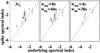 |
Fig. 11 Scatter plot of spectral indices of the spikes versus that of the underlying components using data from 15 keV. |
It is known that flare HXR emission exhibits a harder spectrum at emission peaks than at valleys (e.g., Kiplinger et al. 1983). The spectral analysis for spikes agrees with this general scenario. The different spectral characteristics between fast-varying HXR spikes and underlying components are likely a result of specific physical mechanisms to generate nonthermal emissions in such a way that the spectral properties are closely related to the burst timescales.
3.3. Energy-dependent time delay
We analyzed the time-delay properties of all the spikes detected by different criteria. Four energy bands (25−40, 40−60, 60−100, and 100−300 keV) were used in our analysis. For each spike, we found the peak times τ(ϵ) at different energies relative to the peak time in 25−100 keV. We then performed a least-squares linear-fit between the mean photon energy and τ(ϵ) in logarithmic scale for each spike. If the fitting error was small, we assumed that the spike exhibits a systematic energy-dependent lag in its peak times. Indeed, less than 40% of the spikes evolve with regular time delay patterns, and both low-energy delay and high-energy delay events are detected (note that in Paper I, we only found low-energy delay events). In Fig. 12, we illustrate the distribution of time lags between 60−100 keV and 25−40 keV for these events. In the figure, positive time lags indicate that high-energy emission lags behind low-energy emission, and negative time lags indicate that low-energy emission lags behind high-energy emission. Evidently, the majority of events exhibit time lags shorter than 0.5 s. The mean time lag is about 0.80 s and −0.74 s for high-energy delays and low-energy delays, respectively.
We additionally investigated energy-dependent time lags with respect to the spectral properties for a small fraction of spikes that exhibit a systematic time lag pattern as well as reliable spectral fitting results (Sect. 3.2). For these spikes, we derived spike peak times τ(ϵ) at different energies relative to a reference energy (25−100 keV), and fit τ(ϵ) to an arbitrary function τ(ϵ) ~ ϵα. A positive α indicates that peak emission in higher energies lags behind the peak emission in lower energies, and a negative α indicates lower energy emission lagging behind higher energy emission. The time delay parameter α for different populations of the spikes is shown in Fig. 13. We divided the spikes into two types: low-energy delayed (negative α) and high-energy delayed (positive α). Accordingly, the left part of each panel in Fig. 13 displays the spike spectral index distribution for low-energy delayed events, while the right part shows the distribution for high-energy delayed spikes. In the last panel, the sample number is two, and both of them are low-energy delayed spikes. These figures show that, among these events, about or more than 2/3 are low-energy delayed, and the rest are high-energy delayed. Furthermore, it is found that, on average, high-energy delayed events have a harder count spectrum than low-energy delayed events.
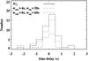 |
Fig. 12 Distributions of spike peak time lags between 60−100 keV and 25−40 keV for spikes selected with various criteria. |
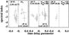 |
Fig. 13 Scatter plot of the spectral index versus the time delay parameter α of spikes selected with various criteria. In each panel, positive α values refer to high-energy delayed events while negative ones refer to low-energy delayed spikes. These two populations are separated by the vertical dashed line, and the number of the spikes, and the mean count spectral index Γ and its standard deviation of each population are also marked in each panel. |
The energy-dependent time lag patterns associated with spike energetics may result from the acceleration and/or transport mechanisms. For example, depending on the initial pitch-angle distribution, when a significant amount of electrons are trapped in the corona, Coulomb collisions in the trap will eject these electrons from the trap to precipitate and lose their energy in the chromosphere. The rate of Coulomb collision is energy-dependent, causing low-energy electrons to precipitate first, thus producing high-energy delayed events. On the other hand, when most electrons are directly precipitated in the chromosphere, the energy-dependent time delays are associated with the electron time of flight, i.e., higher energy electrons with a higher velocity will precipitate ahead of low-energy electrons, accounting for the low-energy delayed events. Our preliminary result showing high-energy delayed events with a harder spectrum indicates that the energetics of HXR spikes are probably coupled with the transport effects, which are, in the first place, governed by acceleration mechanisms determining the electron pitch-angle distribution. A better understanding of the mechanisms that generate these spikes should be obtained from the knowledge of their spatial and magnetic properties.
4. Discussions and conclusions
We have searched all flares observed by RHESSI in 2002 for fast-varying HXR spikes, finding that at least 20% of the flare bursts with count rates exceeding 100 counts s-1 in 25−100 keV produce HXR spikes, mostly during the rise phase of the flares. These spikes have timescales of 0.2−2 s in photon energy range of up to 300 keV. The main results are as follows. (1) Both impulsive and long duration flares can produce HXR spikes with nearly equal production rates. Flares with high peak count rates are more productive in HXR spikes. (2) Almost all spikes occur in the rise phase of the flares, and a large percentage, up to 70%, of spikes are produced at or about the flare peak times. (3) The mean duration of spikes is about 0.9−1.0 s, independent of photon energies. The rise and decay times of spikes are shown to be almost the same. This differs from ordinary flares that usually have a longer decay phase dominated by thermal emission. (4) Most of the spikes can be detected in very high energy bands up to 100−300 keV. The HXR spectra of spikes are harder than those of the underlying slow-varying components. This fact implies the nonthermal origin of spikes. (5) Evident energy-dependent time lags are present in a fraction of spikes, indicative of time-of-flight or Coulomb collision effects. It is also shown that, on average, spikes lagging in high-energy emissions have harder spectra than spikes exhibiting lags in low-energy emissions.
To understand the mechanisms for HXR spikes reported in this study, more observational investigations are needed with substantially improved capabilities or techniques to conduct precise spectral and imaging analyses at the timescales of the spikes.
Acknowledgments
We thank the referee for constructive comments that help improve the presentation. We thank G. J. Hurford for help with the demodulation. Part of this work was conducted during the Research Experience for Undergraduates (REU) program supported by National Science Foundation through grant ATM-0552958 contracted to Montana State University. This work was supported by the Scientific Research Foundation of Graduate School of Nanjing University, FANEDD under grant 200226, NSFC under grants 10878002, 10933003, 11133004 and 11103008, NKBRSF under grant 2011CB811402, the Chinese Academy of Sciences (KZZD-EW-01-3), and US NASA grant NNX08AE44G.
References
- Aschwanden, M. J. 2002, Particle Acceleration and Kinematics in Solar Flares, A Synthesis of Recent Observations and Theoretical Concepts (Dordrecht, Holland: Kluwer Academic Publishers) [Google Scholar]
- Aschwanden, M. J. 2004, Physics of the Solar Corona, An Introduction (Chichester, UK: Praxis Publishing Ltd., Berlin: Springer-Verlag) [Google Scholar]
- Aschwanden, M. J., Schwartz, R. A., & Alt, D. M. 1995, ApJ, 447, 923 [NASA ADS] [CrossRef] [Google Scholar]
- Aschwanden, M. J., Bynum, R. M., Kosugi, T., Hudson, H. S., & Schwartz, R. A. 1997, ApJ, 487, 936 [NASA ADS] [CrossRef] [Google Scholar]
- Bai, T., & Ramaty, R. 1979, ApJ, 227, 1072 [NASA ADS] [CrossRef] [Google Scholar]
- Bespalov, P. A., Zaitsev, V. V., & Stepanov, A. V. 1987, Sol. Phys., 114, 127 [NASA ADS] [Google Scholar]
- Brown, J. C. 1971, Sol. Phys., 18, 489 [NASA ADS] [CrossRef] [Google Scholar]
- Brown, J. C., Conway, A. J., & Aschwanden, M. J. 1998, ApJ, 509, 911 [NASA ADS] [CrossRef] [Google Scholar]
- Carmichael, H. 1964, in Physics of Solar Flares, ed. W. N. Hess (Washington DC: NASA), NASA SP-50, 451 [Google Scholar]
- Correia, E., Costa, J. E. R., Kaufmann, P., Magun, A., & Herrmann, R. 1995, Sol. Phys., 159, 143 [Google Scholar]
- de Jager, C., & de Jonge, G. 1978, Sol. Phys., 58, 127 [NASA ADS] [CrossRef] [Google Scholar]
- Emslie, A. G., & Nagai, F. 1985, ApJ, 288, 779 [NASA ADS] [CrossRef] [Google Scholar]
- Fisher, G. H., Canfield, R. C., & McClymont, A. N. 1985, ApJ, 289, 414 [NASA ADS] [CrossRef] [Google Scholar]
- Furth, H. P., Killeen, J., & Rosenbluth, M. N. 1963, Phys. Fluids, 6, 459 [NASA ADS] [CrossRef] [Google Scholar]
- Hirayama, T. 1974, Sol. Phys., 34, 323 [NASA ADS] [CrossRef] [Google Scholar]
- Hoyng, P., van Beek, H. F., & Brown, J. C. 1976, Sol. Phys., 48, 197 [NASA ADS] [CrossRef] [Google Scholar]
- Kaufmann, P. 1996, Sol. Phys., 169, 377 [NASA ADS] [CrossRef] [Google Scholar]
- Kiplinger, A. L., Dennis, B. R., Frost, K. J., Orwig, L. E., & Emslie, A. G. 1983, ApJ, 265, L99 [NASA ADS] [CrossRef] [Google Scholar]
- Kiplinger, A. L., Dennis, B. R., Frost, K. J., & Orwig, L. E. 1984, ApJ, 287, L105 [NASA ADS] [CrossRef] [Google Scholar]
- Kiplinger, A. L., Dennis, B. R., & Orwig, L. E. 1989, Max ’91 Workshop 2: Developments in Observations and Theory for Solar Cycle 22, eds. R. M. Winglee, & B. R. Dennis (Greenbelt: NASA), 346 [Google Scholar]
- Kliem, B., Karlick, M., & Benz, A. O. 2000, A&A, 360, 715 [NASA ADS] [Google Scholar]
- Kopp, P. A., & Pneuman, G. W. 1976, Sol. Phys., 50, 85 [NASA ADS] [CrossRef] [Google Scholar]
- Lin, R. P., Dennis, B. R., Hurford, G. J., et al. 2002, Sol. Phys., 210, 3 [Google Scholar]
- MacNeice, P., Burgess, A., McWhirter, R. W. P., & Spicer, D. S. 1984, Sol. Phys., 90, 357 [NASA ADS] [CrossRef] [Google Scholar]
- Mariska, J. T., Emslie, A. G., & Li, P. 1989, ApJ, 341, 1067 [NASA ADS] [CrossRef] [Google Scholar]
- Melrose, D. B., & Brown, J. C. 1976, MNRAS, 176, 15 [NASA ADS] [CrossRef] [Google Scholar]
- Priest, E., & Forbes, T. 2000, Magnetic Reconnection (Cambridge, UK: Cambridge University Press) [Google Scholar]
- Qiu, J., Lee, J., & Gary, D. E. 2004, ApJ, 603, 335 [NASA ADS] [CrossRef] [Google Scholar]
- Qiu, J., Cheng, J. X., Hurford, G. J., Xu, Y., & Wang, H. 2012, A&A, 547, A72 (Paper I) [NASA ADS] [CrossRef] [EDP Sciences] [Google Scholar]
- Sturrock, P. A. 1966, Nature, 211, 695 [NASA ADS] [CrossRef] [Google Scholar]
- Sturrock, P. A., & Uchida, Y. 1981, ApJ, 246, 331 [NASA ADS] [CrossRef] [Google Scholar]
- Sturrock, P. A., Kaufman, P., Moore, R. L., & Smith, D. F. 1984, Sol. Phys., 94, 341 [NASA ADS] [CrossRef] [Google Scholar]
- van Beek, H. F., de Feiter, L. D., & de Jager, C. 1974, In Space research XIV, Proc. Sixteenth Plenary Meeting (Berlin, East Germany: Akademie-Verlag GmbH), 447 [Google Scholar]
- van Beek, H. F., de Feiter, L. D., & de Jager, C. 1976, In Space research XVI, Proc. Open Meetings of Working Groups on Physical Sciences (Berlin, East Germany: Akademie-Verlag GmbH), 819 [Google Scholar]
- Vilmer, N., Kane, S. R., & Trottet, G. 1982, A&A, 108, 306 [NASA ADS] [Google Scholar]
All Tables
Spike/flare number variations with σ defined by different combinations of wsmt and wsig and with nsig = 3.
All Figures
|
Fig. 1 Demodulated RHESSI HXR light curves (dark) in comparison with summed raw data counts (gray). The light curves are acquired at 25 − 100 keV. The demodulated light curves correspond to the count rate y-axis and the summed raw data are related to the count y-axis. The top panel shows an event on 2002 March 17 that exhibits fast-varying spikes. The bottom panel shows an event on 2002 February 20 without significant fast-varying spikes. The scales of the raw and demodulated light curves are indicated in the left and right y-axis, respectively. |
| In the text | |
|
Fig. 2 Spike detection algorithm using the three methods (see text) for the event on 2002 August 3. Left panels show the demodulated light curves at 25−100 keV, the slow-varying component (smooth) determined by the three methods, and the residuals (bottom of each panel). The smoothed lines (bottom of each panel) show the sigma levels using the three methods. Right panels show the times (x-axis) and energies (y-axis) of significant residuals recognized by the algorithms. The numbers 1 to 7 along the y-axis indicate energy bands of 10−15, 15−25, 25−40, 40−60, 60−100, 100−300, and 25−100 keV, respectively. The vertical line indicates the most pronounced spikes of the diagrams. |
| In the text | |
|
Fig. 3 Demodulated RHESSI HXR light curves at varying energies for three flares. The vertical lines indicate the spike times. The y-axis gives the units of the 25 − 100 keV light curves, and light curves at other energies are scaled arbitrarily. |
| In the text | |
|
Fig. 4 Number of detected spikes varies as σ level increases. The asterisks and the line represent observational and Poisson distributions, respectively. |
| In the text | |
|
Fig. 5 Peak count rate distributions at various criteria denoted in the figure. The upper thick solid line indicates our 322-flare sample. The profile is obviously steeper than all other profiles. |
| In the text | |
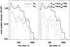 |
Fig. 6 Same as Fig. 3, but for the rise time of flares. |
| In the text | |
|
Fig. 7 Occurrence time τspk distribution at various criteria as denoted in the figure. See Sect. 2.2 for details. |
| In the text | |
|
Fig. 8 ϵhi distribution at various criteria. See Sect. 2.2 for details. |
| In the text | |
|
Fig. 9 Duration τ(ϵ) distributions at various criteria. The average duration is about 0.9−1.0 s in 25−100 keV. See Sect. 3.1 for details. |
| In the text | |
|
Fig. 10 In each panel, the symbols and solid lines show examples of HXR count spectra of integrated spike flux during the spike time in comparison with the count rates spectra of underlying components. Solid lines show the least-squares fit of the spectra to a power-law distribution, and the exponents and their uncertainties from the fit are noted in the figures. The y-axis gives the units of the spike intensities, and the intensities of the underlying component are divided by a number for the clarity of display. S1 is the example we discussed in Fig. 2. |
| In the text | |
|
Fig. 11 Scatter plot of spectral indices of the spikes versus that of the underlying components using data from 15 keV. |
| In the text | |
|
Fig. 12 Distributions of spike peak time lags between 60−100 keV and 25−40 keV for spikes selected with various criteria. |
| In the text | |
|
Fig. 13 Scatter plot of the spectral index versus the time delay parameter α of spikes selected with various criteria. In each panel, positive α values refer to high-energy delayed events while negative ones refer to low-energy delayed spikes. These two populations are separated by the vertical dashed line, and the number of the spikes, and the mean count spectral index Γ and its standard deviation of each population are also marked in each panel. |
| In the text | |
Current usage metrics show cumulative count of Article Views (full-text article views including HTML views, PDF and ePub downloads, according to the available data) and Abstracts Views on Vision4Press platform.
Data correspond to usage on the plateform after 2015. The current usage metrics is available 48-96 hours after online publication and is updated daily on week days.
Initial download of the metrics may take a while.