| Issue |
A&A
Volume 547, November 2012
|
|
|---|---|---|
| Article Number | A91 | |
| Number of page(s) | 16 | |
| Section | Catalogs and data | |
| DOI | https://doi.org/10.1051/0004-6361/201117775 | |
| Published online | 06 November 2012 | |
The Penn State-Toruń Centre for Astronomy Planet Search stars
I. Spectroscopic analysis of 348 red giants⋆,⋆⋆
1
Toruń Centre for Astronomy, Nicolaus Copernicus University,
Gagarina 11,
87-100
Toruń,
Poland
e-mail: This email address is being protected from spambots. You need JavaScript enabled to view it.
; This email address is being protected from spambots. You need JavaScript enabled to view it.
; This email address is being protected from spambots. You need JavaScript enabled to view it.
; This email address is being protected from spambots. You need JavaScript enabled to view it.
2
Department of Astronomy and Astrophysics, Pennsylvania State
University, 525 Davey Laboratory, University Park, PA
16802,
USA
e-mail: This email address is being protected from spambots. You need JavaScript enabled to view it.
3
Center for Exoplanets and Habitable Worlds, Pennsylvania State
University, 525 Davey Laboratory, University Park, PA
16802,
USA
Received: 28 July 2011
Accepted: 21 June 2012
Abstract
Aims. We present basic atmospheric parameters (Teff, log g, vt, and [Fe/H]) as well as luminosities, masses, radii, and absolute radial velocities for 348 stars, presumably giants, from the ~1000 star sample observed within the Penn State-Toruń Centre for Astronomy Planet Search with the High Resolution Spectrograph of the 9.2 m Hobby-Eberly Telescope. The stellar parameters (luminosities, masses, radii) are key to properly interpreting newly discovered low-mass companions, while a systematic study of the complete sample will create a basis for future statistical considerations concerning the appearance of low-mass companions around evolved low- and intermediate-mass stars.
Methods. The atmospheric parameters were derived using a strictly spectroscopic method based on the LTE analysis of equivalent widths of Fe I and Fe II lines. With existing photometric data and the Hipparcos parallaxes, we estimated stellar masses and ages via evolutionary tracks fitting. The stellar radii were calculated from either estimated masses and the spectroscopic log g or from the spectroscopic Teff and estimated luminosities. The absolute radial velocities were obtained by cross-correlating spectra with a numerical template.
Results. We completed the spectroscopic analysis for 332 stars, 327 of which were found to be giants. A simplified analysis was applied to the remaining 16 stars, which had incomplete data. The results show that our sample is composed of stars with effective temperatures ranging from 4055 K to 6239 K, with log g between 1.39 and 4.78 (5 dwarfs were identified). The estimated luminosities are between log L/L⊙ = −1.0 and 3 and lead to masses ranging from 0.6 to 3.4 M⊙. Only 63 stars with masses larger than 2 M⊙ were found. The radii of our stars range from 0.6 to 52 R⊙ with the vast majority between 9−11 R⊙. The stars in our sample are generally less metal-abundant than the Sun with median [Fe/H] = −0.15. The estimated uncertainties in the atmospheric parameters were found to be comparable to those reached in other studies. However, due to lack of precise parallaxes, the stellar luminosities and, in turn, the masses are far less precise, within 0.2 M⊙ in best cases and 0.3 M⊙ on average.
Key words: stars: fundamental parameters / stars: atmospheres / stars: late-type / stars: abundances / planetary systems
Based on observations obtained with the Hobby-Eberly Telescope, which is a joint project of the University of Texas at Austin, Pennsylvania State University, Stanford University, Ludwig-Maximilians-Universität München, and Georg-August-Universität Göttingen.
Tables 1 and 5 are only available at the CDS via anonymous ftp to cdsarc.u-strasbg.fr (130.79.128.5) or via http://cdsarc.u-strasbg.fr/viz-bin/qcat?J/A+A/547/A91
© ESO, 2012
1. Introduction
Since the discovery of the first extrasolar planetary systems by Wolszczan & Frail (1992), Mayor & Queloz (1995), and Marcy & Butler (1996), over 700 planets have been found around other stars. The richness of exoplanets and the architectures of planetary systems emerging today are amazing and raise questions about a general picture of planet formation and evolution. But before such a general picture becomes available, studies of planetary systems in various environments are essential.
The observational techniques applied in searches for exoplanets are all limited to their areas of competence, i.e., the range in stellar or planetary parameters (effective temperatures, masses, planetary periods or orbital separations, etc.) that are available to them. Due to the limitations of current detectors, the direct imaging searches for exoplanets typically deliver massive planets at large orbital distances from low-mass stars (cf. 2M1207 b – Chauvin et al. 2004; or HD 8799 system – Marois et al. 2008). The transit planet searches, conveniently operating in the sini ≈ 1 domain (i being orbital inclination), discover exoplanets with relatively short orbital periods (orbital separations) due to the natural limit of the observable transit length set by the lengths of a night (a condition now being relaxed with the multi-site or space observations, cf. HD 80606 b – Hidas et al. 2010; Hébrard et al. 2010; Kepler 11g – Lissauer et al. 2011). Searches for planets based on the radial velocity (RV) technique are the most versatile. They detect planetary candidates at various orbital separations and in a wide range of planetary minimum masses, as long as sini ≠ 0 (cf. GJ 581 system – Mayor et al. 2009; and 47 UMa d – Gregory & Fischer 2010). Even this method has its limitations, though. Since it requires a large number of narrow spectral lines, it focuses on the slowly rotating cool stars of late-F to M spectral type which sets an upper limit to the main sequence planetary hosts masses (M ≲ 1.5 M⊙). Unfortunately this technique is also seriously affected by the stellar activity (Queloz et al. 2001), which, if not resolved, adds noise (jitter) and limits the precision in RV (Carney et al. 2003; Hekker et al. 2006; Cumming et al. 2008). It is, however, the most suitable in searches for planets around stars more massive than ~1.5 M⊙. In terms of evolution, these stars slow down their rotation and decrease their effective temperatures, becoming red giants available for precise RV measurements.
The Penn State-Toruń Centre for Astronomy Planet Search (PTPS) is aiming to detect and characterize planetary systems around stars at various evolutionary stages (Niedzielski & Wolszczan 2008) with the long-term goal of describing the evolution of planetary systems with aging stars. To this end, over 1000 stars are monitored with the Hobby-Eberly Telescope (HET) for RV variations using the high-precision iodine-cell technique (Butler et al. 1996). The sample is mainly composed of evolved low-mass and intermediate-mass stars: ~575 giants (including 348 stars from the red giant clump (RGC) sample presented here) and ~225 sub-giants, but it also contains ~200 slightly evolved dwarfs. Several stars with planetary-mass companions have already been discovered, mainly around red giants (Niedzielski et al. 2007, 2009a,b; Gettel et al. 2012b,a). These findings supplement the slowly growing population of ~50 planets currently known around evolved stars, discovered in such projects as the McDonald Observatory Planet Search (Cochran & Hatzes 1993; Hatzes & Cochran 1993), the Okayama Planet Search (Sato et al. 2003), the Tautenburg Planet Search (Hatzes et al. 2005), the Lick K-giant Survey (Frink et al. 2002), the ESO FEROS planet search (Setiawan et al. 2003a,b), the Retired A Stars and Their Companions (Johnson et al. 2007), the CORALIE and HARPS search (Lovis & Mayor 2007), and the Boyunsen Planet Search (Lee et al. 2011).
With this paper, we are starting a series devoted to a detailed description of stars incorporated in the complete PTPS sample, their atmospheric parameters, elemental abundances, rotation velocities, kinematical properties, masses, radii, ages, etc. The derived parameters not only describe our sample but also allow for proper interpretation of the planet search results. The stellar masses are essential in extracting minimum masses of the planetary mass companions (mPsini), while the radii and projected rotation velocities are key ingredients in stellar activity considerations etc. Since the complete sample contains ~1000 stars randomly distributed in the skies, it is of interest for general stellar and galactic astrophysics as well. It may be used for studies of galactic structure and evolution, galactic distribution of planetary systems (Haywood 2009), and the galactic habitable zone (Gonzalez et al. 2001; Lineweaver et al. 2004; McCabe & Lucas 2010; Gowanlock et al. 2011).
The paper aims to determine atmospheric parameters, such as effective temperatures (Teff), stellar gravitational accelerations (log g), microturbulence velocities (vt), and metallicities ([Fe/H]) for 348 GK-type stars, presumably red clump giants observed within the PTPS survey. Together with existing photometric data and parallaxes, they will allow us to estimate stellar masses (M/M⊙), radii (R/R⊙), and ages.
The RGC, together with the main sequence (MS) and the red giant branch (RGB), is one of the most characteristic features of the Hertzsprung-Russell diagram (HRD). It was identified by Cannon (1970) and Faulkner & Cannon (1973) as the location of steady-core helium burning. That finding was elaborated in detail by Girardi (1999). Jimenez et al. (1998) used the RGC stars to estimate the age of the Galaxy. Due to very similar intrinsic brightness of all stars at that stage, the RGC was proposed as a standard candle in distance estimates and applied to the Galactic center (Paczynski & Stanek 1998), the Large Magellanic Cloud (Salaris et al. 2003), and other stellar systems.
Their interesting stellar evolution phase and general astrophysical application make the red giants, and especially the RGC stars, the subject of numerous surveys. McWilliam (1990) obtained Teff for 671 stars from broadband photometry, log g via isochrone fitting, and the local thermodynamical equilibrium (LTE) abundances from high-resolution spectra. Zhao et al. (2001) delivered atmospheric parameters, iron abundances, α-element enhancements, and masses for 39 red clump giants selected from the Hipparcos catalogue. Famaey et al. (2005) provided the CORAVEL radial velocities for a sample of about 6600 K-type giants. Detailed spectroscopic studies of various subsamples of the galactic red clump giants were presented in Mishenina et al. (2006), Bizyaev et al. (2006, 2010), Hekker & Meléndez (2007), Liu et al. (2007), Luck & Heiter (2007), Takeda et al. (2008), and Puzeras et al. (2010).
Gontcharov (2008) summarized kinematical properties and galactic distribution of 97 348 RGC stars based on Tycho-2 proper motions and Tycho-2 and 2MASS photometry. Valentini & Munari (2010) studied 277 RGC stars and presented accurate multi-epoch radial velocities, atmospheric parameters, distances, and space velocities (U,V,W). Moreover, Tautvaišienė et al. (2010) in a recent paper presented 12C/13C abundance ratio determinations in a sample of 34 Galactic clump giants as well as abundances of nitrogen, carbon, and oxygen.
Meanwhile, new insight into giants, including clump giants, was gained through CoRoT (Baglin et al. 2006) and Kepler (Gilliland et al. 2010) precise photometry. The solar-like oscillations in red giants were first identified in ground-based RV observations (Hatzes & Cochran 1994; Merline 1999). De Ridder et al. (2009) reported the presence of radial and non-radial oscillations in over 300 giants observed with CoRoT. These oscillations were used in massive masses and radii determinations for giants (Kallinger et al. 2010; Bedding et al. 2010; Hekker et al. 2011).
In Sect. 2 of this paper, we describe the sample and the observational material. The procedure of Fe lines equivalent widths measurements and its precision are presented in Sect. 3. We give the outline of the method applied in our spectroscopic analysis in Sect. 4, while in Sect. 5, we present several tests to evaluate the reliability of the method and estimate uncertainties. Section 6 contains a summary of the atmospheric parameters determined for our stars. These parameters are used in Sect. 7 to estimate stellar integrated parameters: luminosities, masses, radii, and ages. Section 8 presents the method and results of our RV determinations, while a comparison of our results with other published data, is found in Sect. 9. Section 10 discusses atmospheric parameters, and conclusions are presented in Sect. 11.
2. Target selection and observations
The sample of 348 stars presented here constitute the RGC subsample of the PTPS. Originally the SIM-EPIcS1 reference candidates, they were selected as presumable RGC stars due to their photometry and reduced proper motions (Gelino et al. 2005; Law et al. 2006).
They are relatively bright field stars, with V between 4.5 and 11 mag, but in the SIMBAD2 database, spectral types and/or luminosity class estimates are available only for a few (four are classified as dwarfs and 22 as giants). The basic photometric data for the sample stars come from the 2MASS Point Source catalog (Cutri et al. 2003) and the Tycho-2 catalog (Høg & Murdin 2000), compiled by Gelino et al. (2005). For several stars, missing data were gathered from Kharchenko & Roeser (2009). The distributions of visual magnitudes and B − V color indices are presented in Fig. 1. The vast majority, 92% of stars, are fainter than V = 8 mag, with (B − V) between 0.7 and 1.8 mag (1.1 mag on average).
Our sample is composed of much fainter stars than those included in most of the other RGC surveys (Famaey et al. 2005; Mishenina et al. 2006; Hekker & Meléndez 2007; Takeda et al. 2008; Valentini & Munari 2010) and can be compared to the more numerous sample of Bizyaev et al. (2006, 2010). The list of stars, their identification, and basic observational parameters are presented in Table 1.
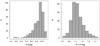 |
Fig. 1 Histograms of the apparent magnitudes in V band (left panel) and (B − V) (right panel) for the 348 red clump giants observed within the PTPS. |
Our high-quality, high-resolution optical spectra have been collected since 2004 with the HET (Ramsey et al. 1998), located in the McDonald Observatory. The telescope was equipped with the High Resolution Spectrograph (HRS) fed with a 2 arcsec fiber, working in the R = 60 000 resolution (Tull 1998). The observations were performed in the queue-scheduled mode (Shetrone et al. 2007). The spectra consisted of 46 echelle orders recorded on the “blue” CCD chip (407−592 nm) and 24 orders on the “red” one (602−784 nm). The signal-to-noise ratio was typically better than 200−250 per resolution element. Basic data reduction (flat fielding, extraction of the spectrum, wavelength calibration, normalization to continuum) was performed using standard IRAF3 tasks and scripts. The wavelength calibration was based on Th-Ar lamp spectrum identification presented in Mader & Shetrone (2002).
3. Equivalent widths of Fe lines
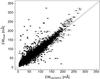 |
Fig. 2 Comparison of the automatic (DAOSPEC) and handmade (IRAF) EWs measurements of 5695 Fe lines for 29 stars. The solid line presents the one-to-one relation, the dashed one is the best linear fit to the data. The individual uncertainties of the DAOSPEC EWs measurements are presented. |
Since equivalent widths (EWs) of hundreds of iron lines for every object were needed, we used the DAOSPEC4 (Stetson & Pancino 2008) to measure the EWs automatically. However, to validate reliability of the results and estimate uncertainties in EWs, we measured the spectra of 29 stars manually with the IRAF (Gaussian fitting) as well. Figure 2 compares the IRAF (manual) with the DAOSPEC (automatic) measurements. We found that the best agreement between the measurements is reached for lines with EWs lower than 200 mÅ. Lines with larger EWs revealed some discrepancy towards higher manual EWs values. In general, the linear fit to all measurements is nearly a one-to-one relation. For 5632 lines with the EW ≤ 200 mÅ, we found EWIRAF = (0.937 ± 0.005)EWDAOSPEC + (8.46 ± 0.35) and the Pearson correlation coefficient of R = 0.939. The mean difference between the IRAF and the DAOSPEC measurements was 5.3 mÅ with a scatter of 12.8 mÅ. The mean uncertainty in the DAOSPEC EWs was 2.13 mÅ. We proceeded with the automatic measurements in the further analysis.
To apply the procedure described in the following section, we measured the EWs of neutral (Fe I) and ionized (Fe II) iron absorption lines for which precise atomic data, i.e., laboratory wavelengths, lower excitation potentials (χ), and oscillator strength (gf) were available from Takeda et al. (2005a,b). All these atomic data were compiled from the line-lists of Grevesse & Sauval (1999), Meylan et al. (1993), and Kurucz et al. (1984). Due to differences in the spectral coverage and CCD chip cosmetics, we were able to identify up to 296 lines (269 Fe I and 27 Fe II lines) from the initial sample of ~330 iron lines from Takeda et al. (2005a) in the HET/HRS spectra. After rejecting blends as well as very weak and saturated lines, we used the EWs of 190 Fe I and 15 Fe II lines per star on average. Only unblended lines with the EWs ranging from 5 mÅ to 200 mÅ were included in the final spectroscopic analysis.
4. An outline of the analysis method
The iron EWs were analyzed with the TGVIT (Takeda et al. 2002a, 2005a), which is a part of the SPTOOL5 package. This numerical algorithm is a modified version of an earlier code and is based on the atmospheric models computed by Kurucz (1993a,b). The TGVIT uses an iterative procedure to achieve more cohesive parameter fits, and the version available to us was more suitable for lower effective temperatures (Teff ≥ 4250 K) than the original version (Takeda et al. 2002a). As a result, we could apply it to the late-type stars in our sample. More details concerning the iteration procedures, data calculations, and formulation of the numerical problems are presented in Takeda et al. (2002a,b, 2005a,b).
This purely spectroscopic method is based on an analysis of Fe I and Fe II lines and fulfills three conditions resulting from the assumption of the local thermodynamical equilibrium (LTE):
-
1.
the abundances derived from Fe I lines maynot show any dependence on the lower excitationpotential χ (excitation equilibrium);
-
2.
the averaged abundances from Fe I and Fe II lines must be equal (ionization equilibrium);
-
3.
the abundances derived from Fe I lines may not show any dependence on the EWs (matching the curve of growth shape).
We used the TGVIT to calculate Teff, log g, vt, and [Fe/H], defined in the standard manner as [Fe/H] = log (NFe/NH) − log (NFe/NH)⊙, with the solar value of 7.50 (Kurucz 1993a; Holweger et al. 1991).
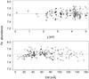 |
Fig. 3 Illustration of the TGVIT analysis of TYC 3018-00996-1: Fe abundance vs. χ (top panel) relation and Fe abundance vs. EW (bottom panel) relation. The open and filled circles stand for 176 Fe I and 12 Fe II lines respectively. The mean Fe abundance is shown on each panel as a dashed line. |
Because of the relatively low Teff of our stars, the number of available Fe II lines was not sufficiently large (less than 10% of Fe I lines). Consequently, we neglected the dispersion of Fe II abundances while estimating the minimization function D2 (TGVIT defines the dispersion D2 as a function of three arguments: Teff, log g, and vt that is minimized to obtain proper Fe abundance). For the coefficients included in D2, we assumed the values of c1 = 0, c2 = 1, c3 = 0 (see Takeda et al. 2002a, for details).
In the vast majority of cases, all three above-mentioned conditions were fulfilled. This was checked for every star by visual evaluation of relations between Fe abundances and χ or EWs like those presented in Fig. 3. The assumptions were justified if no relation between Fe abundance and these two parameters was present. Other conditions evaluated for every star were the equivalence of mean Fe abundances for Fe I and Fe II lines and the scatter around average abundance. After visual inspection, the Fe lines showing apparent deviations from the mean Fe abundances were rejected. In the following step, the parameters were redetermined and the procedure was repeated until coherent solutions for all parameters were reached. The rejected lines were typically unrecognized blends or lines with EWs larger than 150 mÅ and the excitation potential of less than 0.5 eV.
The Fe abundance depends on both Teff and log g. The coupling is so strong that in the iterative approach of Takeda et al. (2002a)Teff and log g are actually simultaneously fitted and treated as “one variable” (vt being the other). This coupling may, in principle, lead to degeneracy of purely spectroscopic parameters because higher effective temperatures may be compensated by gravitational acceleration. However, in our sample, which is composed of stars with effective temperatures similar or lower to the Sun, we do not expect this effect to cause significant uncertainties. We refer the reader to Takeda et al. (2002a) for a detailed discussion of this problem and for an extensive discussion on the behavior of the D2 function, along with its related components, around the converged solutions.
5. Verification of the adopted approach
Atmospheric parameters of the Sun and τ Cet determined by Takeda et al. (2005a) and our results.
Atmospheric parameters determined by Soubiran et al. (1998) and our results for 13 stars observed with ELODIE.
Before running the TGVIT for our program stars, we performed a series of tests using various input data. First of all, we tested our installation of the TGVIT by running it with the data for the Sun and τ Cet (HD 10700) distributed together with the code. These EWs were obtained from high-dispersion spectra obtained at the Okayama Astrophysical Observatory with the 188 cm telescope (Takeda et al. 2005a). Our results are compared with those of Takeda et al. (2005a) in Table 2. The results are practically identical, which proves that our installation works well.
In the next step, we determined atmospheric parameters (i) for several stars, for which similar determinations were available from Katz et al. (1998), using Echelle spectra available from the ELODIE Library (Soubiran et al. 1998) and (ii) for a few well-known stars with planets, for which recent atmospheric parameter determinations are available in Butler et al. (2006), using our own HET/HRS spectra. The purpose of these tests was to estimate reliability of the adopted method and to search for systematic effects.
Another important reason for that analysis was to assess the reliability of uncertainties delivered by the TGVIT as these are determined from the quality of fits for Teff, log g, and microturbulence velocity and should be considered intrinsic. Only the uncertainties in [Fe/H] are based on actual scatter between individual determinations for all lines in use and are expected to be realistic.
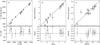 |
Fig. 4 Comparison of the atmospheric parameters for 13 stars observed with the ELODIE. The panels present the relations (top) and differences (bottom) between our results and those obtained by Soubiran et al. (1998) for Teff (a), log g (b), and [Fe/H] (c). The solid lines represent one-to-one relations. |
5.1. Tests with ELODIE data
With the TGVIT, we analyzed the spectra of 13 randomly selected stars, downloaded from the ELODIE Library (Soubiran et al. 1998)6 at the Observatoire de Haute-Provence. Both giants and dwarfs with spectral types of G0-K3 were selected to cover parameter space similar to our sample.
These spectra were obtained with a resolution of R = 42 000 (Katz et al. 1998), which was lower than ours. The spectral wavelength range covered was 390−680 nm in 67 Echelle orders. Typical signal-to-noise ratio was 100−150 per pixel. The spectra were reduced, i.e., straightened, wavelength-calibrated, and cleaned from cosmic ray hits, bad pixels, and telluric lines. Because of the narrower spectral range, we were able to measure 150 Fe I and 15 Fe II lines per star on average for the further analysis.
The results obtained with the TGVIT for these 13 stars are presented and compared with results of Soubiran et al. (1998) in Table 3 and Fig. 4.
Atmospheric parameters taken from Butler et al. (2006) and our results for eight planet-hosting stars.
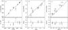 |
Fig. 5 Comparison of the atmospheric parameters for eight known planet-hosting stars. Both relations (top) and differences (bottom) between our results and those of Butler et al. (2006) of Teff (a), log g (b), and [Fe/H] (c) are presented. The one-to-one relations are presented as solid lines. |
The mean intrinsic uncertainties of our determinations are σTeff = 21 K, σlog g = 0.07, and σ[Fe/H] = 0.09. According to Katz et al. (1998), the average uncertainties based on the internal accuracy assumed for stars with a signal-to-noise ratio around 100 are σTeff = 86 K, σlog g = 0.28, and σ[Fe/H] = 0.16. We note that the mean intrinsic uncertainties in Teff and log g as given by the TGVIT are about four times smaller than uncertainties estimated by Katz et al. (1998), while in the case of [Fe/H] they are comparable. An overall agreement of the results is clear from Fig. 4.
We calculated the mean differences and scatter (rms) between our results and those of Soubiran et al. (1998) (excluding HD 175305, for which uncertainties in Soubiran et al. 1998, are much larger than typical) and obtained ΔTeff = 63 K, Δlog g = 0.15, Δ[Fe/H] = 0.02, σDTeff = 54 K, σDlog g = 0.27, and σD[Fe/H] = 0.25.
Since we used exactly the same spectra as Soubiran et al. (1998), the only sources of the differences in the results and estimated uncertainties are the numerical procedures, the selection of lines, and the EW measurements. We note that our intrinsic uncertainties in Teff, log g are 2.6−3.8 times smaller than the resulting scatter in the results. We also note that our results for Teff are systematically 63 K (3σ) larger, while our results for log g are systematically 0.15 dex (2.1σ) estimated larger. However, the [Fe/H] results do not show any systematical effects as compared with Soubiran et al. (1998). The scatter in all results, which is comparable to uncertainties as determined from Katz et al. (1998) and, especially in [Fe/H], is larger than the average uncertainty as estimated by Katz et al. (1998), suggests that our results are more precise than those of Soubiran et al. (1998).
5.2. Tests with Butler et al. (2006) data
We performed another test on the quality and reliability of our results using our own HET/HRS spectra of eight known hosts of planetary systems: HD 10697, HD 38529, HD 72659, HD 74156, HD 75732, HD 88133, HD 118203, and HD 209458, previously analyzed by other authors. The sample contained mainly dwarfs and sub-giants, with spectral types ranging from F8 to K0. Our results were compared to the determinations collected in Butler et al. (2006), who included the nearby stars and exoplanets data from the Lick, the Keck, and the Anglo-Australian Observatory planet searches. The results of our analysis for the eight planet-hosting stars are summarized in Table 4, where the atmospheric parameters from Butler et al. (2006) are also presented (see Fig. 5). The mean intrinsic uncertainties for the atmospheric parameters we obtained and present in Table 4 are σTeff = 15 K, σlog g = 0.04, and σ[Fe/H] = 0.06, while the uncertainties presented by Butler et al. (2006) are σTeff = 55 K, σlog g = 0.06, and σ[Fe/H] = 0.03. The mean intrinsic uncertainties in Teff as given by the TGVIT are 3.6 times smaller than estimated uncertainties given in Butler et al. (2006), while our estimated uncertainties in the log g and the [Fe/H] are comparable.
After rejecting HD 118203, for which the uncertainty in Teff as given in Butler et al. (2006) is three times larger than average, we calculated the mean differences and scatter (rms) between our results and those collected in Butler et al. (2006). We obtained ΔTeff = −31 K, Δlog g = −0.02, Δ[Fe/H] = −0.08, σDTeff = 49 K, σDlog g = 0.12, and σD[Fe/H] = 0.05.
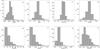 |
Fig. 6 Distributions of atmospheric parameters for the 332 stars with complete spectroscopic analysis: Teff, log g, vt, and [Fe/H] (panels a)−d)) and their intrinsic uncertainties (panels e)−h)). |
Our intrinsic uncertainties in Teff and log g are 3.3 and three times smaller, respectively, than the resulting scatter in the results. The scatter in [Fe/H] is similar to our uncertainty estimate.
We note that our results for Teff and [Fe/H] are systematically smaller by 31 K (2σ) and 0.08 dex (1.3σ), respectively, while the results for log g do not show any measurable systematical effects as compared with Butler et al. (2006). The scatter among all results is comparable to uncertainties determined by Butler et al. (2006) and by us, especially in [Fe/H], where it is smaller than our estimate. This suggests that the results presented in Butler et al. (2006) are of similar quality or more accurate than ours.
In concluding our tests, we note that in general the Teff, log g, and [Fe/H] obtained with the TGVIT and those selected from Soubiran et al. (1998) or Butler et al. (2006) agree with each other. The uncertainties in the metallicities, estimated in the TGVIT from the actual Fe abundance distribution as the standard deviation of the mean, are realistic. Our [Fe/H] determinations agree with those of Soubiran et al. (1998), but are systematically 1.3σ lower than those presented in Butler et al. (2006).
The intrinsic TGVIT uncertainties of Teff are most certainly underestimated. The comparison with results from Soubiran et al. (1998) suggests that we should increase our σTeff estimates by a factor of 2.6. Similar analysis of scatter between our data and those of Butler et al. (2006) suggests that our uncertainties are underestimated by a factor of 3.3. If we apply such corrected σCTeff = 3.3σTeff estimate, our results agree with those of Soubiran et al. (1998) and Butler et al. (2006) within 1σC. Similar analysis of scatter leads to the conclusion that our σlog g estimates should be increased by a factor of three. With such uncertainty estimates our log g determinations also agree with those of both Soubiran et al. (1998) and Butler et al. (2006) well within σClog g = 3.0σlog g. Since the microturbulence velocity uncertainty is estimated in the same manner as for Teff and log g, we expect that these uncertainties are also underestimated by a factor of three.
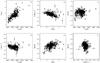 |
Fig. 7 Relations between Teff, log g, vt, and [Fe/H] for the 332 stars with complete spectroscopic analysis. The uncertainties in all cases are presented. |
6. Atmospheric parameters
The results of our determinations of the atmospheric parameters for 348 GK giant stars are presented in Table 5 (Cols. 2−5). In all cases, the values of Teff, log g, vt, and [Fe/H] are presented together with their intrinsic uncertainties. For 332 objects, we obtained consistent solutions for each of the stellar parameters in (typically) ten iterations of the procedure described in Sect. 4.
The spectroscopic analysis revealed that five of our presumable giants are actually dwarfs (TYC 0435-01209-1, TYC 0683-01063-1, TYC 1496-01002-1, TYC 3012-00273-1, and TYC 4444-00200-1) with log g ≥ 4.0. On the other hand, four objects (TYC 2818-00449-1, TYC 2818-00504-1, TYC 2823-01028-1, and TYC 2823-01398-1) recognized in the SIMBAD as dwarfs are actually K-type giants.
The values of Teff, log g, vt, and [Fe/H] for 332 stars were found to stay generally within the range of the TGVIT model grids. However, analysis of 24 stars resulted in effective temperatures below 4250 K with other parameters within the TGVIT range of applicability. As the Kurucz (1993a) models included in the TGVIT reach down to 4000 K, we consider these determinations to be realistic but associated with larger uncertainties, as will be illustrated in Sect. 6.1. For 16 stars, the resulting atmospheric parameters were either incoherent or outside the range of applicability of the TGVIT. A simplified analysis was performed for these stars, as described in Sect. 6.2, and they will be discussed separately.
The obtained Teff ranges between 4055 K and 6239 K with a median value at 4736 K. The distribution of Teff is presented in Fig. 6a. Virtually all our stars have Teff between 4000 K and 5200 K (with the vast majority, ~200, between 4600 K and 5000 K), making them mostly G8-K2 stars. The five dwarfs are among the hottest stars in our sample, with Teff between 4906 K and 6239 K. The intrinsic uncertainty distribution in Teff is presented in Fig. 6e.
The derived log g for our sample stars ranges between 1.39 and 4.78, with the median of 2.66. The distribution of log g is presented in Fig. 6b. The majority of our stars (251) have log g of 2.0−3.0, making them generally giants. Small fractions of 19 bright giants with log g ≤ 2.0 and 3 subgiants with 3.7 ≤ log g ≤ 4.0 are present in our sample as well. The intrinsic uncertainty distribution in log g is presented in Fig. 6f.
The resulting microturbulence velocity reaches values from 0.57 km s-1 to 2.49 km s-1 and has a median value of 1.4 km s-1. Most of our stars have vt between 1.2 km s-1 and 1.6 km s-1 (Fig. 6c). The value of vt for five dwarfs in our sample is scattered over the range 0.57−1.68 km s-1. The intrinsic uncertainty distribution of vt is presented in Fig. 6g.
The metallicity of stars in our sample, [Fe/H], stays within −1.0 to + 0.45 range, with a median value of −0.15. Figure 6d presents the distribution and shows that our stars are generally less metal-abundant than the Sun, with most of them having [Fe/H] in the range of −0.5 to 0.0. The intrinsic uncertainty distribution in [Fe/H] is presented in Fig. 6h.
Figure 7 presents a few relations between purely spectroscopic atmospheric parameters presented in Table 5. They illustrate a general resemblance of our sample to those studied by others (cf. Takeda et al. 2008). In Fig. 7a, one can notice a clear dependance of log g on Teff. The log g tends to be higher for hotter stars. For stars with Teff ≳ 5000 K, the dispersion in surface gravity increases with effective temperature as well. Noticeable relations exist between vt and both log g and Teff (Figs. 7b and d). The vt decreases with both log g and Teff. In general, [Fe/H] values seem to be significantly lower for low log g stars (Fig. 7e) in our sample, while they reveal uniform distributions in Teff (Fig. 7c) and vt (Fig. 7f).
6.1. Uncertainty estimates
The mean intrinsic uncertainties of our determinations were found to be σTeff = 13 K, σlog g = 0.05, σvt = 0.08 km s-1, and σ[Fe/H] = 0.07. As discussed in Sect. 5, all these uncertainties, except [Fe/H], are numerical, resulting from the iterative procedures of the TGVIT. The real uncertainties are factor of three larger (since our intrinsic uncertainty scaling may change in a comparison with a larger reference sample, we present our intrinsic uncertainties instead of the scaled ones). In the case of [Fe/H], the numerical uncertainties are the standard deviation of the mean Fe I and Fe II abundances, hence realistic. The distributions of the intrinsic uncertainties are preseneted in Fig. 6 (panels e−h). There exists no correlation between the intrinsic uncertainties and the parameter values obtained for any of the atmospheric parameters. The scatter of the intrinsic uncertainties is also uniformly distributed over the respective parameters values, but it is worth noting that for the stars with Teff below 4250 K, the intrinsic uncertainties are higher, especially in log g and [Fe/H]. In Fig. 8, the intrinsic uncertainties of Teff, log g, and [Fe/H] as a function of Teff are presented.
Several stars from the sample demonstrate uncertainties of atmospheric parameters at least two times larger than the mean values. In the case of [Fe/H], we noted intrinsic uncertainties larger than 0.12 for six stars (TYC 0870-00241-1, TYC 1425-01506-1, TYC 3012-01520-1, TYC 3304-00408-1, TYC 4006-00980-1, and TYC 4428-01582-1). These result from the highest scatter of Fe abundances with respect to the excitation potential and EWs in the whole sample.
Five objects (TYC 0096-00005-1, TYC 1425-01506-1, TYC 3011-00791-1, TYC 3304-00408-1, and TYC 3930-01790-1) have significantly larger Teff intrinsic uncertainties (≥ 30 K). In the case of log g larger than typical intrinsic uncertainty (>0.1) was obtained for nine stars (TYC 0096-00005-1, TYC 0276-00507-1, TYC 0870-00241-1, TYC 1425-01506-1, TYC 3012-01520-1, TYC 3304-00405-1, TYC 3304-00408-1, TYC 3930-01790-1, and TYC 4006-00980-1). The precision in vt is the worst (i.e., ≥ 0.15 km s-1) for eight objects (TYC 0683-01063-1, TYC 0870-00084-1, TYC 1425-01506-1, TYC 1496-01002-1, TYC 3011-00791-1, TYC 3012-00273-1, TYC 3930-01790-1, and TYC 4444-00200-1).
The reason for such increases in uncertainty is not always clear. For some stars, it may be associated with low effective temperatures close to the TGVIT model grids limit of Teff = 4250 K (TYC 0096-0005-1, TYC 1425-01506-1, TYC 3304-00405-1, TYC 3304-00408-1, TYC 0276-00507-1, TYC 3012-01520-1). In several other cases, the relatively low signal-to-noise ratio of our spectra might be the reason (TYC 3011-00791-1, TYC 4006-00980-1, TYC 0870-00084-1, TYC 1496-01002-1, TYC 3012-00273-1, TYC 4444-00200-1, TYC 4428-01582-1).
It is also possible that the larger-than-expected uncertainties may be due to an unresolved stellar companion. This is the case with TYC 0870-00241-1, a star with excellent quality spectra and all atmospheric parameters well within the TGVIT range: after several epochs of PTPS RV monitoring, it appeared to have a stellar-mass companion (Niedzielski et al., in prep.).
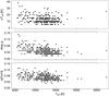 |
Fig. 8 Relations between the intrinsic uncertainties of σTeff (top panel), σlog g (middle panel), and σ[Fe/H] (bottom panel) vs. Teff for 332 PTPS stars. |
6.2. Stars with incomplete data
Sixteen stars of our sample have atmospheric parameters that are difficult to derive using the Takeda et al. (2005a) method. For these stars, the solutions found with the TGVIT were either inconsistent or unrealistic. To include at least some of these stars in our analysis, we adopted Teff, log g, and initial luminosity estimates from Adamów et al. (in prep.) for all of them. Effective temperatures were calculated from the empirical calibration of Ramírez & Meléndez (2005), based on Tycho and 2MASS photometry. Rough estimates of log g were obtained using the results of Bilir et al. (2006) and Gelino et al. (2005). For all these stars, the average value of [Fe/H] obtained for the 332 stars with complete spectroscopic analysis, [Fe/H] = −0.15, was assumed (bottom part of Table 5).
This approach revealed that three stars were indeed too cool for the approach of Takeda et al. (2005a,b). The remaining 13 did not show any different characteristics in comparison with the 332 stars with complete spectroscopic analysis, and the reasons why they were not applicable to the TGVIT remain to be clarified. Due to the much larger uncertainty of adopted atmospheric parameters for these stars, they will be either discussed separately or not considered in the following sections.
7. Luminosities, masses, ages, and radii
For 271 stars from our sample, no Hipparcos parallaxes are available and for another four (TYC 0017-01084-1, TYC 3663-00622-1, TYC 4006-00019-1, and TYC 3304-00090-1), the Hipparcos parallaxes π are unreliable (σπ ≥ π). As a result, only estimates of masses and radii based on spectrophotometric parallaxes derived here are possible in most cases. For such estimates, bolometric luminosities are required in addition to our log g, Teff, and metallicities. We calculated the intrinsic color index (B − V)0 and the bolometric corrections BCV for our stars from the empirical calculation of Alonso et al. (1999). Using photometry and assuming standard interstellar reddening with R = 3.1 (Rieke & Lebofsky 1985), we estimated luminosities for 57 stars with usable parallaxes. For 275 objects with unknown or unreliable Hipparcos parallaxes, we initially assumed MV from the empirical calculation of Straizys & Kuriliene (1981) and estimated luminosities on that basis.
Propagation of uncertainty was applied to estimate luminosity uncertainty. The adopted luminosities, together with their uncertainty estimates, are presented in Table 5 (Col. 11). For the 57 stars with reliable parallaxes, the values obtained here were adopted (the last column in Table 1 identifies the stars with the Hipparcos parallaxes). For the remaining 275 stars, luminosities were constrained better via fitting to evolutionary tracks, as described in the following section.
7.1. Stellar masses and luminosities
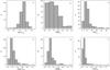 |
Fig. 9 Distributions of luminosities, masses, and radii (panels a)−c)) as well as their uncertainties (panels d)−f)) for 332 stars with complete spectroscopic analysis. |
The stellar masses M/M⊙, the radii R/R⊙, and the estimates of ages were obtained by comparing the positions of stars in the [log L/L⊙, log g, log Teff] space with the theoretical evolutionary tracks of Girardi et al. (2000) and Salasnich et al. (2000) for a given metallicity (Fig. 10). We used all available tracks corresponding to eight metallicity values: [Y = 0.23,Z = 0.0004], [Y = 0.23,Z = 0.001], [Y = 0.24,Z = 0.004], [Y = 0.25,Z = 0.008], [Y = 0.273,Z = 0.019] (the solar composition), [Y = 0.30,Z = 0.03], [Y = 0.32,Z = 0.04], and [Y = 0.39,Z = 0.07]. To derive M/M⊙ for every star, the tracks for the nearest metallicity were applied. Then the maximum-likelihood function defined as 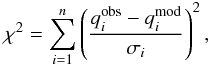 (1)where
  ,
,  , and σi denote observed and modeled parameters and their uncertainties respectively, was minimized over the model parameter space. In our case, the number of parameters n was set to three because log L/L⊙, log g, and log Teff were used. The area over which the parameter space was explored was defined as ± 10σ (intrinsic) in log g and log Teff and as ± 3σ in log L/L⊙. The resulting run of the χ2 over the model parameters was found to be typically relatively flat. Therefore, the final stellar mass was calculated as a mean value over an extended area of
  . Using that procedure, we could determine consistent stellar masses and realistically evaluate the uncertainties.
The resulting masses range from 0.6 M/M⊙ to 3.4 M/M⊙ (see Fig. 9b for a histogram). The majority of stars in our sample have masses below 2 M⊙. We identified, however, a significant number (63 or ~19%) of stars that fall in the intermediate-mass range of 2 M⊙ ≤ M ≤ 7 M⊙. Table 5 (Col. 12) presents the final adopted masses.
The uncertainty of stellar mass obtained by comparison with the theoretical evolutionary tracks selected here (Girardi et al. 2000; Salasnich et al. 2000) depends on how accurately the position of a star in the [log L/L⊙, log g, log Teff] space is determined. The effective temperatures and gravities are relatively well determined, and the largest source of uncertainty is the parallax, i.e., luminosity. In the case of stars for which the parallax π was precise enough, choosing the metallicity model may cause additional uncertainty since we used the existing evolutionary tracks.
For an average red giant with known parallax, we found that the mass may be estimated within 0.2 M⊙ in the best cases, while the mean uncertainty for the whole sample is σM/M⊙ = 0.3. The uncertainties may become even larger, ~1 M⊙, for very confused evolutionary tracks regions at lower effective temperatures (log Teff ≤ 3.65).
No reliable parallaxes were available for most of our stars. As a result, luminosity log L/L⊙ was constrained better than the initial estimate by adopting the luminosity from the fits to the evolutionary tracks, corresponding to the determined log g, log Teff, and the stellar mass. In Table 5 (Col. 11), such luminosity estimates are presented for 275 stars. The log L/L⊙ ranges from −0.68 to 2.86, with a peak at 1.6 (Fig. 9a). The mean uncertainty in log L/L⊙ was found to be 0.19 in the best cases, but the average value for the whole sample is σlog L/L⊙ = 0.23.
The H-R diagram for 332 PTPS stars with the complete spectroscopic analysis is presented in Fig. 10.
7.2. Age estimates
As a large number of the stars presented have roughly solar masses, a small uncertainty in mass leads to significant uncertainties in the resulting age. However, for the intermediate-mass stars, the precision in mass is worse but the estimated ages are more robust. The ages of the majority of our program stars are therefore uncertain. The estimated stellar ages are presented in Table 5 (Col. 14). A wide range is given for many stars, reflecting the complex nature of RGC region and the difficulties in age determination for single field objects. Nevertheless, we found that a typical star from our sample is 3−5 Gyr old (mean uncertainty in age is 1.1−1.5 Gyr).
7.3. Stellar radii
The stellar radii were estimated from either spectroscopic log g and the adopted stellar mass or from spectroscopic Teff and the adopted luminosity. In every case, a parameter obtained from the spectroscopic analysis and one from the model fitting were used according to the equations 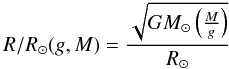 (2)or
(2)or 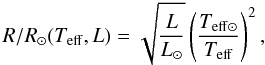 (3)where G is the gravitational constant and M⊙, R⊙, L⊙, and Teff ⊙ are the solar values of mass, radius, luminosity, and effective temperature.
Maximum uncertainty was estimated in both approaches by applying the logarithmic derivative method. In Fig. 11, a comparison of radii derived using both methods is presented. Although the radii differ significantly for several stars, the general agreement between both R/R⊙ estimates is good. The mean absolute difference between radii determined from Eqs. (2) and (3) is ΔR = 0.7 R⊙. The largest deviations exist for the most extended stars (cf. Fig. 11). They most probably result from inaccurate luminosity estimates for those luminous stars without parallax and from a departure from LTE conditions in stars with the most extended outer regions. Due to better consistency with the evolutionary status, the radii obtained from Eq. (3) are given in Table 5 (Col. 13), along with their uncertainties.
The radii of stars in our sample range from 0.6 R⊙ to 52.1 R⊙ (Fig. 9c), with the majority between 9−11 R⊙. The mean uncertainty in the derived stellar radii was found to be 0.8 R/R⊙ (Fig. 9f).
7.4. Stars with incomplete data
For the 16 stars with incomplete atmospheric data discussed in Sect. 6.2 and presented in the bottom part of the Table 5, we applied essentially the same procedure to obtain luminosities, masses, ages, and radii. However, as only rough estimates of log g and assumed [Fe/H] were available, the resulting masses, ages, and radii are very uncertain. Therefore, we excluded these 16 stars from our discussion in Sect. 10.
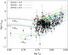 |
Fig. 10 H-R diagram for 332 PTPS stars with the complete spectroscopic analysis. The theoretical evolutionary tracks (Girardi et al. 2000) are presented for stellar masses of 1−3 M⊙ and several metallicities. The dotted, solid, and dashed lines correspond to [Fe/H] = −0.4,0.0,0.3, respectively. |
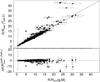 |
Fig. 11 Comparison of radii obtained from two sets of stellar parameters: log g, M/M⊙ and Teff, log L/L⊙ for 332 stars. The solid line corresponds to one-to-one relation. |
8. Radial velocities
A cross-correlation analysis with an artificial template was applied to obtain absolute radial velocities. To construct the cross-correlation functions (CCFs), the normalized stellar spectra were correlated with a numerical mask consisting of 1 and 0 value points (Nowak & Niedzielski 2008). The nonzero points corresponded to the positions of 300 nonblended, isolated stellar absorption lines at zero velocity. In our RV measurements, only the first 17 orders of the “blue” spectra, free from telluric lines, were used. The CCF was computed step by step for each velocity point without merging the orders. For every order, the algorithm selected only lines suitable for a given wavelength range. The CCFs from all orders were finally added to construct the final CCF for the whole spectrum. The final radial velocities were measured by fitting a Gaussian function to the CCF for the whole spectrum. The uncertainties of the RVs were computed as rms of the 17 RVs obtained from fitting a Gaussian to the CCF for each order separately. The mean standard uncertainty obtained this way was σRVCCF = 0.041 km s-1. In Fig. 12, the distribution of resulting RVs and their uncertainties is presented. The absolute precision of presented RV is lower than the σRVCCF. The HRS is neither thermally nor pressure stabilized. As a result, the wavelength scale of our spectra is affected by these factors, and the real uncertainties are likely to be of the order of 1 km s-1.
Table 5 (Cols. 6−8) presents the RVs transformed to the barycenter of the Solar System with the algorithm of Stumpff (1980) for all stars in our sample (except for TYC 3304-00479-1, due to the lack of suitable spectra), together with the epochs of observation (MJD).
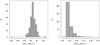 |
Fig. 12 Histograms of the RVs obtained from the cross-correlation function (left panel) and their uncertainties (right panel) for 347 stars. |
9. Comparison with literature data
Because the vast majority of our stars were studied here for the first time, no comparison with literature data is possible. Nevertheless, several individual objects were included in other surveys, so we can compare our results with those of other authors, obtained with various methods.
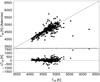 |
Fig. 13 Comparison of Teff of the 332 PTPS stars obtained in this study and taken from Adamów et al. (in prep.). Both relation (top) and differences (bottom) are presented. The uncertainties of both determinations are shown. The solid line corresponds to one-to-one relation. |
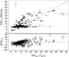 |
Fig. 14 Comparison of the R/R⊙ for the 332 PTPS stars derived here and calculated from the empirical calibration of Alonso et al. (2000). Both relation (top) and differences (bottom) are presented. The uncertainties in our determinations are shown for every target, whereas for Alonso et al. (2000) radii a typical uncertainty for 10 R⊙ star is denoted in the upper left corner. The solid line presents the one-to-one relation. |
The spectroscopic determinations of Teff were compared with effective temperatures derived by Adamów et al. (in prep.) from the empirical calibration of Ramírez & Meléndez (2005) and the Tycho and the 2MASS photometry, where all our stars were included. The comparison of results for 332 stars is shown in Fig. 13. No significant systematic shift is present in the data, but the scatter of 224 K on average increases towards higher effective temperatures. The mean difference between our temperature and those of Adamów et al. (in prep.) is ΔTeff = 48 K; only for four objects is the difference significantly larger (>740 K). These stars are TYC 0683-01063-1, TYC 3319-00170-1, TYC 3930-00665-1, and TYC 3993-01850-1. They are all significantly reddened by the interstellar extinction, which probably affected the photometric Teff.
Our adopted values of stellar radii for 332 stars were compared with estimates obtained from the empirical calibration of Alonso et al. (2000), based on the angular diameters attained from the infrared flux method and distances computed from the Hipparcos parallaxes. In most cases, the results of R/R⊙ were fairly close to each other and comparable within the estimated uncertainties. It is worth mentioning that uncertainties in radii as estimated from the calibration of Alonso et al. (2000) are large, and only a typical uncertainty for a 10 R⊙ star is presented in Fig. 14. The mean difference between our radii and calibrated radii is Δ(R/R⊙) = −2.2 with a scatter of 5.8 R⊙. It is interesting to note that our estimates give systematically lower values for the stars with smaller radii, and systematically larger ones for the stars with larger radii. This is most probably caused by the departure from the LTE.
In Fig. 15, we present a collective comparison of our parameters for several stars with the data available in the literature. The results obtained by other authors agree, in general, with our determinations of Teff, log g, [Fe/H], and R/R⊙. In spite of a very low number of stars in common, i.e., five for Teff, four for log g, eight for [Fe/H], and five for R/R⊙, the agreement is obvious, especially in the case of metallicity. It appears from Fig. 15, however, that the scatter between the determinations of various authors is large, which makes the comparison more difficult.
In Fig. 16, the RVs obtained using the CCF technique are compared with literature data for all stars, for which such determinations were available. In all but three cases, our radial velocities agree with those of other authors. Large discrepancies exist in TYC 3012-02518-1, TYC 3930-01790-1, and TYC 3304-00090-1. The first two stars are members of binary systems (Abt 1981; Meisel 1968), where the latter is in addition chromospherically active (e.g., Strassmeier 1994). The reason for absolute RV discrepancy for TYC 3304-00090-1 is discussed in more detail in Adamów et al. (2012).
The mean differences between the respective parameters are summarized in Table 6. We found that on average our determinations agree with all presented literature results within ΔTeff = −6 K, Δlog g = 0.07, Δ[Fe/H] = −0.07, ΔR/R⊙ = −0.6, and ΔRV = −0.029 km s-1 (with the exception of the three discrepant stars). The mean scatter of these comparisons represented by the standard deviation is equal to 179 K, 0.76 dex, 0.10 dex, 3.8 R⊙, and 0.841 km s-1 for Teff, log g, [Fe/H], R, and RV, respectively. No systematic effects were found. Our results agree with those of other authors within the estimated uncertainties.
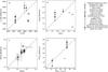 |
Fig. 15 Comparison of various parameters for stars with the literature data. The uncertainties are presented if available. The solid lines denote the one-to-one relations. |
Mean differences and standard deviations between stellar parameters presented in this work and derived by other authors.
10. Discussion
Several relations between the integral and the atmospheric parameters are depicted in Fig. 17. From the mass−luminosity relation (Fig. 17a), we infer that relatively high-mass stars tend to be brighter. In the case of solar-mass objects, however, we see a large dispersion in log L/L⊙. A clear correlation exists between log L/L⊙ and log R/R⊙ (Fig. 17b), reflecting the well-known relation  . In Fig. 17c, a strong log R/R⊙ dependance on log g, resulting from Eq. (2), is visible. One can also see that the hotter stars in our sample tend to be of higher mass (Fig. 17d), except for the dwarfs, which reveal similar masses for a wide range of effective temperatures (~1300 K). These effects are largely a result of our sample definition, which is well illustrated in the log L/L⊙ vs. log Teff relation (Fig. 10). In turn, masses of our sample stars show quite uniform distribution versus log g and [Fe/H] (Figs. 17e and f).
In Fig. 17g, we see that our stars are quite uniformly distributed over the metallicity vs. radius plane. Figure 17h is similar to the mass−luminosity relation (Fig. 17a), probably because the stellar radii presented in Fig. 17b result from the derived luminosities.
The age−metallicity relation for 332 PTPS stars is shown in Fig. 18 (top panel). As we stated in Sect. 7.2, the stellar ages are uncertain and in many cases were ambiguously determined. The lower limit of log Age is presented if the age range is given in Table 5 (Col. 14). However, the well-known tendency resulting from the Galactic evolution is maintained. In Fig. 18 (bottom panel), the relation between stellar age and mass is presented (the Pearson correlation coefficient is R = −0.937). A quadratic fit can be determined for stars with masses larger than the solar mass: M/M⊙ = (1.07 ± 0.07)(log Age)2−(21.42 ± 1.30)(log Age) + (107.93 ± 6.04). Based Fig. 18, we find that the giants in our sample present a wide range of evolutionary stages. Relatively older stars (≥ 3.2 Gyr) have simultaneously lower masses (~1 M⊙) and reveal a higher spread in metallicity (0.26). The more massive giants (>1.5 M⊙), with lower spread in metallicity (0.16), are younger (<3.2 Gyr).
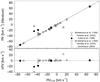 |
Fig. 16 Radial velocities derived from our cross-correlation analysis compared with those available in the literature. Relation (top) and differences (bottom) between the RV results are shown. The uncertainties of the RVs are presented if available. The solid line presents the one-to-one relation. |
From Fig. 10, one can see that our sample is composed mainly of regular giants evolving along the RGB and giants from the RGC. Only very few stars appeared to be dwarfs. We applied the definitions of RGC as proposed in Jimenez et al. (1998) and Tautvaisiene & Puzeras (2009), i.e., 4700 K ≤ Teff ≤ 5100 K and 1.5 ≤ log L/L⊙ ≤ 1.8 to our data. Due to the large uncertainty in our luminosities, we extended the log L/L⊙ range by 0.2 to [1.3−2.0]. As a result, we found 126 stars to fulfill the criteria for the clump giants. These stars constitute only about 38% of our sample. The mean absolute magnitudes of these stars in four bands (MV = (0.985 ± 0.499) mag, MJ = (− 0.700 ± 0.502) mag, MH = (− 1.178 ± 0.502) mag, and MK = (− 1.282 ± 0.508) mag) confirm that they are the clump giants. In Fig. 19, we can see our RGC stars together with the rest of the sample in MK vs. Teff and MK vs. [Fe/H] plots. The scatter (defined as the standard deviation) in the absolute magnitudes is large due to the lack of parallaxes, and it is not possible to search for relations with either metallicity or temperature. Given the observational uncertainties in luminosity and our sample definition, we cannot state that the observed relative frequency of RGC stars reflects the true one.
The stellar masses obtained here by fitting observed stellar parameters to selected evolutionary tracks are model dependent. Since the mass-loss was ignored, they also should be considered as upper limits.
11. Conclusions
We presented the atmospheric parameters (Teff, log g, vt, and [Fe/H]), luminosities, masses, radii, ages, and absolute radial velocities for 348 stars from the RGC sample of the PTPS. For the vast majority of them, these are the first determinations.
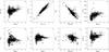 |
Fig. 17 Relations between log L/L⊙, M/M⊙, log R/R⊙ and the atmospheric parameters for the 332 stars with complete spectroscopic analysis. The uncertainties in all cases are presented. |
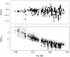 |
Fig. 18 Relations between [Fe/H] and log Age (top panel) as well as M/M⊙ and log Age (bottom panel) for the 332 stars with complete spectroscopic analysis. Only the uncertainties in [Fe/H] and M/M⊙ are presented. The lower limit of log Age is presented if the age range is given in Table 5 (Col. 14). |
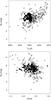 |
Fig. 19 Relations between MK and Teff (top panel) as well as MK and [Fe/H] (bottom panel) for 327 giants. The RGC stars are presented as solid circles, while the rest of stars are shown as open circles. |
For 332 stars, the complete spectroscopic analysis resulted in precise Teff, log g, vt, and metallicities. The intrinsic uncertainties in the parameters derived are σTeff = 13 K, σlog g = 0.05, σvt = 0.08 km s-1, and σ[Fe/H] = 0.07 (the uncertainties in effective temperatures, gravities and microturbulence velocities as discussed in Sect. 5 are underestimated by a factor of three). In the case of 16 stars, for which either data was incomplete or our spectroscopic approach failed, effective temperatures and log g were estimated from the photometric data.
In our analysis, five stars from the present sample appeared to be dwarfs and 343 giants, 126 of which are located in the red clump. Our RGC sample was found to be composed of stars with Teff between 4055 K and 6239 K and a median value at 4736 K (with majority, ~200 of them, between 4600 K and 5000 K), generally G8-K2 stars. The log g determined ranges between 1.39 and 4.78 with a median of 2.66 (the majority of our stars, 251, have log g of 2.0−3.0) making them generally giants. A small fraction of 19 bright giants with log g ≤ 2.0 and three subgiants with 3.7 ≤ log g ≤ 4.0 is present as well. The microturbulence velocity, vt, for stars from this sample ranges from 0.57 km s-1 to 2.49 km s-1 and has a median at 1.4 km s-1. The metallicity, [Fe/H], of stars in our RGC sample stays within −1.0 to + 0.45 range. With a median of −0.15, our stars are generally less metal abundant than the Sun, and most of them have [Fe/H] in the range of −0.5−0.0.
For all 348 stars, luminosities, masses, radii and ages were estimated using the atmospheric parameters presented, archive photometric data and the Hipparcos parallaxes, when available. The log L/L⊙ ranges from −0.68 to 2.86 with the maximum peak at 1.6. The resulting masses range from 0.6 M/M⊙ to 3.4 M/M⊙, with the majority of stars having masses below 2 M⊙. We identified, however, 63 (or ~19%) stars that fall in the intermediate-mass range 2 M⊙ ≤ M ≤ 7 M⊙. The radii determined range from 0.6 R⊙ to 52.1 R⊙. Most of our stars have radii of about 9−11 R⊙. We found that stars from our sample are typically 3−5 Gyr old and have mean uncertainties in age of around 1.1−1.5 Gyr. Average uncertainties in derived parameters are σlog L/L⊙ = 0.23, σM = 0.3 M⊙, σR = 0.8 R⊙.
We find the precision in stellar parameters derived acceptable for the main purpose of our project, i.e., a massive planet search. The precision of atmospheric parameters allows for more sophisticated analysis of individual stars in future. However, since the lack of the Hipparcos parallaxes was identified as the main source of the uncertainty in luminosities, masses, radii, and ages for most of our stars, we expect that the Gaia7 satellite (Lindegren et al. 1994; Perryman et al. 1997; Bailer-Jones 2002) will enable to constrain the intrinsic parameters better.
Space Interferometry Mission (SIM) key project: Extra-solar Planet Interferometric Survey (EPIcS) http://planetquest.jpl.nasa.gov/SIM
The SIMBAD astronomical database is operated at CDS, Strasbourg, France.
IRAF is distributed by the National Optical Astronomy Observatories, which are operated by the Association of Universities for Research in Astronomy, Inc., under cooperative agreement with the National Science Foundation.
Library of the ELODIE spectra of F5 to K7 stars is only available in electronic form via http://vizier.cfa.harvard.edu/viz-bin/VizieR?-source=J/A+AS/133/221
Global Astrometric Interferometer for Astrophysics (Gaia) is a European Space Agency (ESA) space mission to be launched in 2013.
Acknowledgments
We thank Dr. Yoichi Takeda as well as Dr. Peter Stetson and Dr. Elena Pancino for making their codes available to us. We thank the HET resident astronomers and telescope operators for their continuous support. We also thank anonymous referees for comments and suggestions that helped us to improve the manuscript. P.Z., A.N., M.A., and G.N. were supported in part by the Polish Ministry of Science and Higher Education grants N N203 510938, and N N203 386237. A.W. was supported by the NASA grant NNX09AB36G. The Hobby-Eberly Telescope (HET) is a joint project of the University of Texas at Austin, Pennsylvania State University, Stanford University, Ludwig-Maximilians-Universität München, and Georg-August-Universität Göttingen. The HET is named in honor of its principal benefactors, William P. Hobby and Robert E. Eberly. The Center for Exoplanets and Habitable Worlds is supported by Pennsylvania State University, the Eberly College of Science, and the Pennsylvania Space Grant Consortium. This research has made extensive use of the SIMBAD database, operated at CDS (Strasbourg, France), and NASA’s Astrophysics Data System Bibliographic Services.
References
- Abt, H. A. 1981, ApJS, 45, 437 [NASA ADS] [CrossRef] [Google Scholar]
- Adamów, M., Niedzielski, A., Villaver, E., Nowak, G., & Wolszczan, A. 2012, ApJ, 754, L15 [NASA ADS] [CrossRef] [Google Scholar]
- Alonso, A., Arribas, S., & Martínez-Roger, C. 1999, A&AS, 140, 261 [NASA ADS] [CrossRef] [EDP Sciences] [Google Scholar]
- Alonso, A., Salaris, M., Arribas, S., Martínez-Roger, C., & Asensio Ramos, A. 2000, A&A, 355, 1060 [NASA ADS] [Google Scholar]
- Baglin, A., Auvergne, M., Barge, P., et al. 2006, in The CoRoT Mission Pre-Launch Status – Stellar Seismology and Planet Finding, eds. M. Fridlund, A. Baglin, J. Lochard, & L. Conroy (European Space Agency), ESA SP, 1306, 33 [Google Scholar]
- Bailer-Jones, C. A. L. 2002, Ap&SS, 280, 21 [NASA ADS] [CrossRef] [Google Scholar]
- Baines, E. K., McAlister, H. A., ten Brummelaar, T. A., et al. 2009, ApJ, 701, 154 [NASA ADS] [CrossRef] [Google Scholar]
- Baines, E. K., Döllinger, M. P., Cusano, F., et al. 2010, ApJ, 710, 1365 [NASA ADS] [CrossRef] [Google Scholar]
- Balachandran, S., Lambert, D. L., & Stauffer, J. R. 1988, ApJ, 333, 267 [NASA ADS] [CrossRef] [Google Scholar]
- Bartkevičius, A., & Sperauskas, J. 1999, Baltic Astron., 8, 325 [NASA ADS] [Google Scholar]
- Bedding, T. R., Huber, D., Stello, D., et al. 2010, ApJ, 713, L176 [NASA ADS] [CrossRef] [Google Scholar]
- Bilir, S., Karaali, S., Güver, T., Karataş, Y., & Ak, S. G. 2006, Astron. Nachr., 327, 72 [NASA ADS] [CrossRef] [Google Scholar]
- Bizyaev, D., Smith, V. V., Arenas, J., et al. 2006, AJ, 131, 1784 [NASA ADS] [CrossRef] [Google Scholar]
- Bizyaev, D., Smith, V. V., & Cunha, K. 2010, AJ, 140, 1911 [NASA ADS] [CrossRef] [Google Scholar]
- Blackwell, D. E., & Lynas-Gray, A. E. 1998, A&AS, 129, 505 [NASA ADS] [CrossRef] [EDP Sciences] [Google Scholar]
- Bordé, P., Coudé du Foresto, V., Chagnon, G., & Perrin, G. 2002, A&A, 393, 183 [NASA ADS] [CrossRef] [EDP Sciences] [Google Scholar]
- Brown, J. A., Sneden, C., Lambert, D. L., & Dutchover, Jr., E. 1989, ApJS, 71, 293 [CrossRef] [Google Scholar]
- Butler, R. P., Marcy, G. W., Williams, E., et al. 1996, PASP, 108, 500 [NASA ADS] [CrossRef] [Google Scholar]
- Butler, R. P., Wright, J. T., Marcy, G. W., et al. 2006, ApJ, 646, 505 [NASA ADS] [CrossRef] [Google Scholar]
- Cannon, R. D. 1970, MNRAS, 150, 111 [NASA ADS] [CrossRef] [Google Scholar]
- Carney, B. W., Latham, D. W., Stefanik, R. P., Laird, J. B., & Morse, J. A. 2003, AJ, 125, 293 [NASA ADS] [CrossRef] [Google Scholar]
- Chauvin, G., Lagrange, A.-M., Dumas, C., et al. 2004, A&A, 425, L29 [NASA ADS] [CrossRef] [EDP Sciences] [MathSciNet] [Google Scholar]
- Cochran, W. D., & Hatzes, A. P. 1993, in Planets Around Pulsars, eds. J. A. Phillips, S. E. Thorsett, & S. R. Kulkarni (San Francisco: ASP), ASP Conf. Ser., 36, 267 [Google Scholar]
- Cumming, A., Butler, R. P., Marcy, G. W., et al. 2008, PASP, 120, 531 [CrossRef] [Google Scholar]
- Cutri, R. M., Skrutskie, M. F., van Dyk, S., et al. 2003, VizieR Online Data Catalog, II/246 [Google Scholar]
- de Medeiros, J. R., & Mayor, M. 1999, A&AS, 139, 433 [NASA ADS] [CrossRef] [EDP Sciences] [Google Scholar]
- De Ridder, J., Barban, C., Baudin, F., et al. 2009, Nature, 459, 398 [Google Scholar]
- Duflot, M., Figon, P., & Meyssonnier, N. 1995, A&AS, 114, 269 [NASA ADS] [Google Scholar]
- Famaey, B., Jorissen, A., Luri, X., et al. 2005, A&A, 430, 165 [NASA ADS] [CrossRef] [EDP Sciences] [Google Scholar]
- Faulkner, D. J., & Cannon, R. D. 1973, ApJ, 180, 435 [NASA ADS] [CrossRef] [Google Scholar]
- Frink, S., Mitchell, D. S., Quirrenbach, A., et al. 2002, ApJ, 576, 478 [NASA ADS] [CrossRef] [MathSciNet] [Google Scholar]
- Gelino, C. R., Shao, M., Tanner, A. M., & Niedzielski, A. 2005, in Protostars and Planets V, eds. B. Reipurth, D. Jewitt, & K. Keil (Houston: Lunar and Planetary Institute), LPI Contribution, 1286, 8602 [Google Scholar]
- Gettel, S., Wolszczan, A., Niedzielski, A., et al. 2012a, ApJ, 756, 53 [Google Scholar]
- Gettel, S., Wolszczan, A., Niedzielski, A., et al. 2012b, ApJ, 745, 28 [NASA ADS] [CrossRef] [Google Scholar]
- Gilliland, R. L., Brown, T. M., Christensen-Dalsgaard, J., et al. 2010, PASP, 122, 131 [NASA ADS] [CrossRef] [Google Scholar]
- Girardi, L. 1999, MNRAS, 308, 818 [NASA ADS] [CrossRef] [MathSciNet] [Google Scholar]
- Girardi, L., Bressan, A., Bertelli, G., & Chiosi, C. 2000, A&AS, 141, 371 [NASA ADS] [CrossRef] [EDP Sciences] [Google Scholar]
- Gontcharov, G. A. 2006, Astron. Lett., 32, 759 [NASA ADS] [CrossRef] [Google Scholar]
- Gontcharov, G. A. 2008, Astron. Lett., 34, 785 [NASA ADS] [CrossRef] [Google Scholar]
- Gonzalez, G., Brownlee, D., & Ward, P. 2001, Icarus, 152, 185 [NASA ADS] [CrossRef] [Google Scholar]
- Gowanlock, M. G., Patton, D. R., & McConnell, S. M. 2011, Astrobiology, 11, 855 [NASA ADS] [CrossRef] [Google Scholar]
- Gregory, P. C., & Fischer, D. A. 2010, MNRAS, 403, 731 [NASA ADS] [CrossRef] [Google Scholar]
- Grevesse, N., & Sauval, A. J. 1999, A&A, 347, 348 [NASA ADS] [Google Scholar]
- Hatzes, A. P., & Cochran, W. D. 1993, ApJ, 413, 339 [NASA ADS] [CrossRef] [Google Scholar]
- Hatzes, A. P., & Cochran, W. D. 1994, ApJ, 432, 763 [NASA ADS] [CrossRef] [Google Scholar]
- Hatzes, A. P., Guenther, E. W., Endl, M., et al. 2005, A&A, 437, 743 [NASA ADS] [CrossRef] [EDP Sciences] [Google Scholar]
- Haywood, M. 2009, ApJ, 698, L1 [NASA ADS] [CrossRef] [Google Scholar]
- Hébrard, G., Désert, J.-M., Díaz, R. F., et al. 2010, A&A, 516, A95 [NASA ADS] [CrossRef] [EDP Sciences] [Google Scholar]
- Hekker, S., & Meléndez, J. 2007, A&A, 475, 1003 [NASA ADS] [CrossRef] [EDP Sciences] [Google Scholar]
- Hekker, S., Reffert, S., Quirrenbach, A., et al. 2006, A&A, 454, 943 [NASA ADS] [CrossRef] [EDP Sciences] [Google Scholar]
- Hekker, S., Gilliland, R. L., Elsworth, Y., et al. 2011, MNRAS, 414, 2594 [Google Scholar]
- Hidas, M. G., Tsapras, Y., Mislis, D., et al. 2010, MNRAS, 406, 1146 [NASA ADS] [Google Scholar]
- Høg, E., & Murdin, P. 2000, Tycho Star Catalogs: The 2.5 Million Brightest Stars (Bristol: IOP) [Google Scholar]
- Holweger, H., Bard, A., Kock, M., & Kock, A. 1991, A&A, 249, 545 [NASA ADS] [Google Scholar]
- Jimenez, R., Flynn, C., & Kotoneva, E. 1998, MNRAS, 299, 515 [NASA ADS] [CrossRef] [Google Scholar]
- Johnson, J. A., Fischer, D. A., Marcy, G. W., et al. 2007, ApJ, 665, 785 [NASA ADS] [CrossRef] [Google Scholar]
- Kallinger, T., Mosser, B., Hekker, S., et al. 2010, A&A, 522, A1 [NASA ADS] [CrossRef] [EDP Sciences] [Google Scholar]
- Katz, D., Soubiran, C., Cayrel, R., Adda, M., & Cautain, R. 1998, A&A, 338, 151 [NASA ADS] [Google Scholar]
- Kharchenko, N. V., & Roeser, S. 2009, VizieR Online Data Catalog, I/280 [Google Scholar]
- Kurucz, R. 1993a, ATLAS9 Stellar Atmosphere Programs and 2 km s-1 grid, Kurucz CD-ROM No. 13 (Cambridge, Mass.: Smithsonian Astrophysical Observatory) [Google Scholar]
- Kurucz, R. 1993b, SYNTHE Spectrum Synthesis Programs and Line Data, Kurucz CD-ROM No. 18 (Cambridge, Mass.: Smithsonian Astrophysical Observatory) [Google Scholar]
- Kurucz, R. L., Furenlid, I., Brault, J., & Testerman, L. 1984, Solar flux atlas from 296 to 1300 nm (New Mexico: National Solar Observatory) [Google Scholar]
- Law, N. M., Tanner, A., Kulkarni, S., Shao, M., & Gelino, C. 2006, BAAS, 38, 1227 [NASA ADS] [Google Scholar]
- Lee, B.-C., Mkrtichian, D. E., Han, I., Kim, K.-M., & Park, M.-G. 2011, A&A, 529, A134 [NASA ADS] [CrossRef] [EDP Sciences] [Google Scholar]
- Lindegren, L., Perryman, M. A., Bastian, U., et al. 1994, in Proc. SPIE, 2200, 599 [Google Scholar]
- Lineweaver, C. H., Fenner, Y., & Gibson, B. K. 2004, Science, 303, 59 [NASA ADS] [CrossRef] [Google Scholar]
- Lissauer, J. J., Fabrycky, D. C., Ford, E. B., et al. 2011, Nature, 470, 53 [NASA ADS] [CrossRef] [PubMed] [Google Scholar]
- Liu, Y. J., Zhao, G., Shi, J. R., Pietrzyński, G., & Gieren, W. 2007, MNRAS, 382, 553 [NASA ADS] [CrossRef] [Google Scholar]
- Lovis, C., & Mayor, M. 2007, A&A, 472, 657 [NASA ADS] [CrossRef] [EDP Sciences] [Google Scholar]
- Luck, R. E. 1991, ApJS, 75, 579 [NASA ADS] [CrossRef] [Google Scholar]
- Luck, R. E., & Heiter, U. 2007, AJ, 133, 2464 [NASA ADS] [CrossRef] [Google Scholar]
- Mader, J., & Shetrone, M. D. 2002, in HET Technical Document No. 300 (University of Texas, McDonald Observatory) [Google Scholar]
- Marcy, G. W., & Butler, R. P. 1996, ApJ, 464, L147 [NASA ADS] [CrossRef] [Google Scholar]
- Marois, C., Macintosh, B., Barman, T., et al. 2008, Science, 322, 1348 [NASA ADS] [CrossRef] [PubMed] [Google Scholar]
- Mayor, M., & Queloz, D. 1995, Nature, 378, 355 [NASA ADS] [CrossRef] [Google Scholar]
- Mayor, M., Bonfils, X., Forveille, T., et al. 2009, A&A, 507, 487 [NASA ADS] [CrossRef] [EDP Sciences] [Google Scholar]
- McCabe, M., & Lucas, H. 2010, Int. J. Astrobiol., 9, 217 [CrossRef] [Google Scholar]
- McWilliam, A. 1990, ApJS, 74, 1075 [NASA ADS] [CrossRef] [Google Scholar]
- Meisel, D. D. 1968, AJ, 73, 350 [NASA ADS] [CrossRef] [Google Scholar]
- Merline, W. J. 1999, in Precise Stellar Radial Velocities, eds. J. B. Hearnshaw, & C. D. Scarfe (San Francisco: ASP), ASP Conf. Ser., 185, 187 [Google Scholar]
- Meylan, T., Furenlid, I., Wiggs, M. S., & Kurucz, R. L. 1993, ApJS, 85, 163 [NASA ADS] [CrossRef] [Google Scholar]
- Mishenina, T. V., Bienaymé, O., Gorbaneva, T. I., et al. 2006, A&A, 456, 1109 [NASA ADS] [CrossRef] [EDP Sciences] [Google Scholar]
- Nidever, D. L., Marcy, G. W., Butler, R. P., Fischer, D. A., & Vogt, S. S. 2002, ApJS, 141, 503 [NASA ADS] [CrossRef] [Google Scholar]
- Niedzielski, A., & Wolszczan, A. 2008, in Exoplanets: Detection, Formation and Dynamics, eds. Y.-S. Sun, S. Ferraz-Mello, & J.-L. Zhou (Cambridge: CUP), IAU Symp., 249, 43 [Google Scholar]
- Niedzielski, A., Konacki, M., Wolszczan, A., et al. 2007, ApJ, 669, 1354 [NASA ADS] [CrossRef] [Google Scholar]
- Niedzielski, A., Goździewski, K., Wolszczan, A., et al. 2009a, ApJ, 693, 276 [NASA ADS] [CrossRef] [Google Scholar]
- Niedzielski, A., Nowak, G., Adamów, M., & Wolszczan, A. 2009b, ApJ, 707, 768 [NASA ADS] [CrossRef] [Google Scholar]
- Nordgren, T. E., Germain, M. E., Benson, J. A., et al. 1999, AJ, 118, 3032 [NASA ADS] [CrossRef] [Google Scholar]
- Nowak, G., & Niedzielski, A. 2008, in Extreme Solar Systems, eds. D. Fischer, F. A. Rasio, S. E. Thorsett, & A. Wolszczan (San Francisco: ASP), ASP Conf. Ser., 398, 173 [Google Scholar]
- Paczynski, B., & Stanek, K. Z. 1998, ApJ, 494, L219 [NASA ADS] [CrossRef] [Google Scholar]
- Pasinetti Fracassini, L. E., Pastori, L., Covino, S., & Pozzi, A. 2001, A&A, 367, 521 [NASA ADS] [CrossRef] [EDP Sciences] [Google Scholar]
- Perryman, M. A. C., Lindegren, L., & Turon, C. 1997, in Hipparcos – Venice ’97, eds. R. M. Bonnet, E. Høg, P. L. Bernacca, et al. (European Space Agency), ESA SP, 402, 743 [Google Scholar]
- Puzeras, E., Tautvaišienė, G., Cohen, J. G., et al. 2010, MNRAS, 408, 1225 [NASA ADS] [CrossRef] [Google Scholar]
- Queloz, D., Henry, G. W., Sivan, J. P., et al. 2001, A&A, 379, 279 [NASA ADS] [CrossRef] [EDP Sciences] [Google Scholar]
- Ramírez, I., & Meléndez, J. 2005, ApJ, 626, 446 [NASA ADS] [CrossRef] [MathSciNet] [Google Scholar]
- Ramsey, L. W., Adams, M. T., Barnes, T. G., et al. 1998, in Proc. SPIE, 3352, 34 [Google Scholar]
- Rieke, G. H., & Lebofsky, M. J. 1985, ApJ, 288, 618 [NASA ADS] [CrossRef] [Google Scholar]
- Salaris, M., Percival, S., & Girardi, L. 2003, MNRAS, 345, 1030 [NASA ADS] [CrossRef] [Google Scholar]
- Salasnich, B., Girardi, L., Weiss, A., & Chiosi, C. 2000, A&A, 361, 1023 [NASA ADS] [Google Scholar]
- Sato, B., Ando, H., Kambe, E., et al. 2003, ApJ, 597, L157 [NASA ADS] [CrossRef] [Google Scholar]
- Setiawan, J., Hatzes, A. P., von der Lühe, O., et al. 2003a, A&A, 398, L19 [NASA ADS] [CrossRef] [EDP Sciences] [Google Scholar]
- Setiawan, J., Pasquini, L., da Silva, L., von der Lühe, O., & Hatzes, A. 2003b, A&A, 397, 1151 [NASA ADS] [CrossRef] [EDP Sciences] [Google Scholar]
- Shetrone, M., Cornell, M. E., Fowler, J. R., et al. 2007, PASP, 119, 556 [NASA ADS] [CrossRef] [Google Scholar]
- Soubiran, C., Katz, D., & Cayrel, R. 1998, A&AS, 133, 221 [NASA ADS] [CrossRef] [EDP Sciences] [Google Scholar]
- Soubiran, C., Bienaymé, O., Mishenina, T. V., & Kovtyukh, V. V. 2008, A&A, 480, 91 [NASA ADS] [CrossRef] [EDP Sciences] [Google Scholar]
- Stetson, P. B., & Pancino, E. 2008, PASP, 120, 1332 [Google Scholar]
- Straizys, V., & Kuriliene, G. 1981, Ap&SS, 80, 353 [NASA ADS] [CrossRef] [Google Scholar]
- Strassmeier, K. G. 1994, A&AS, 103, 413 [NASA ADS] [Google Scholar]
- Stumpff, P. 1980, A&AS, 41, 1 [NASA ADS] [Google Scholar]
- Takeda, Y., Ohkubo, M., & Sadakane, K. 2002a, PASJ, 54, 451 [NASA ADS] [CrossRef] [Google Scholar]
- Takeda, Y., Sato, B., Kambe, E., Sadakane, K., & Ohkubo, M. 2002b, PASJ, 54, 1041 [NASA ADS] [Google Scholar]
- Takeda, Y., Ohkubo, M., Sato, B., Kambe, E., & Sadakane, K. 2005a, PASJ, 57, 27 [NASA ADS] [CrossRef] [Google Scholar]
- Takeda, Y., Sato, B., Kambe, E., et al. 2005b, PASJ, 57, 109 [Google Scholar]
- Takeda, Y., Sato, B., & Murata, D. 2008, PASJ, 60, 781 [NASA ADS] [CrossRef] [Google Scholar]
- Tautvaisiene, G., & Puzeras, E. 2009, in The Galaxy Disk in Cosmological Context, eds. J. Andersen, J. Bland-Hawthorn, & B. Nordström (Cambridge: CUP), IAU Symp., 254, 75 [Google Scholar]
- Tautvaišienė, G., Edvardsson, B., Puzeras, E., Barisevičius, G., & Ilyin, I. 2010, MNRAS, 409, 1213 [NASA ADS] [CrossRef] [Google Scholar]
- Taylor, B. J. 1999, A&AS, 134, 523 [NASA ADS] [CrossRef] [EDP Sciences] [Google Scholar]
- Tull, R. G. 1998, in Proc. SPIE, 3355, 387 [Google Scholar]
- Valentini, M., & Munari, U. 2010, A&A, 522, A79 [NASA ADS] [CrossRef] [EDP Sciences] [Google Scholar]
- van Belle, G. T., & von Braun, K. 2009, ApJ, 694, 1085 [NASA ADS] [CrossRef] [Google Scholar]
- Wolszczan, A., & Frail, D. A. 1992, Nature, 355, 145 [NASA ADS] [CrossRef] [Google Scholar]
- Zhao, G., Qiu, H. M., & Mao, S. 2001, ApJ, 551, L85 [NASA ADS] [CrossRef] [Google Scholar]
All Tables
Atmospheric parameters of the Sun and τ Cet determined by Takeda et al. (2005a) and our results.
Atmospheric parameters determined by Soubiran et al. (1998) and our results for 13 stars observed with ELODIE.
Atmospheric parameters taken from Butler et al. (2006) and our results for eight planet-hosting stars.
Mean differences and standard deviations between stellar parameters presented in this work and derived by other authors.
All Figures
|
Fig. 1 Histograms of the apparent magnitudes in V band (left panel) and (B − V) (right panel) for the 348 red clump giants observed within the PTPS. |
| In the text | |
|
Fig. 2 Comparison of the automatic (DAOSPEC) and handmade (IRAF) EWs measurements of 5695 Fe lines for 29 stars. The solid line presents the one-to-one relation, the dashed one is the best linear fit to the data. The individual uncertainties of the DAOSPEC EWs measurements are presented. |
| In the text | |
|
Fig. 3 Illustration of the TGVIT analysis of TYC 3018-00996-1: Fe abundance vs. χ (top panel) relation and Fe abundance vs. EW (bottom panel) relation. The open and filled circles stand for 176 Fe I and 12 Fe II lines respectively. The mean Fe abundance is shown on each panel as a dashed line. |
| In the text | |
|
Fig. 4 Comparison of the atmospheric parameters for 13 stars observed with the ELODIE. The panels present the relations (top) and differences (bottom) between our results and those obtained by Soubiran et al. (1998) for Teff (a), log g (b), and [Fe/H] (c). The solid lines represent one-to-one relations. |
| In the text | |
|
Fig. 5 Comparison of the atmospheric parameters for eight known planet-hosting stars. Both relations (top) and differences (bottom) between our results and those of Butler et al. (2006) of Teff (a), log g (b), and [Fe/H] (c) are presented. The one-to-one relations are presented as solid lines. |
| In the text | |
|
Fig. 6 Distributions of atmospheric parameters for the 332 stars with complete spectroscopic analysis: Teff, log g, vt, and [Fe/H] (panels a)−d)) and their intrinsic uncertainties (panels e)−h)). |
| In the text | |
|
Fig. 7 Relations between Teff, log g, vt, and [Fe/H] for the 332 stars with complete spectroscopic analysis. The uncertainties in all cases are presented. |
| In the text | |
|
Fig. 8 Relations between the intrinsic uncertainties of σTeff (top panel), σlog g (middle panel), and σ[Fe/H] (bottom panel) vs. Teff for 332 PTPS stars. |
| In the text | |
|
Fig. 9 Distributions of luminosities, masses, and radii (panels a)−c)) as well as their uncertainties (panels d)−f)) for 332 stars with complete spectroscopic analysis. |
| In the text | |
|
Fig. 10 H-R diagram for 332 PTPS stars with the complete spectroscopic analysis. The theoretical evolutionary tracks (Girardi et al. 2000) are presented for stellar masses of 1−3 M⊙ and several metallicities. The dotted, solid, and dashed lines correspond to [Fe/H] = −0.4,0.0,0.3, respectively. |
| In the text | |
|
Fig. 11 Comparison of radii obtained from two sets of stellar parameters: log g, M/M⊙ and Teff, log L/L⊙ for 332 stars. The solid line corresponds to one-to-one relation. |
| In the text | |
|
Fig. 12 Histograms of the RVs obtained from the cross-correlation function (left panel) and their uncertainties (right panel) for 347 stars. |
| In the text | |
|
Fig. 13 Comparison of Teff of the 332 PTPS stars obtained in this study and taken from Adamów et al. (in prep.). Both relation (top) and differences (bottom) are presented. The uncertainties of both determinations are shown. The solid line corresponds to one-to-one relation. |
| In the text | |
|
Fig. 14 Comparison of the R/R⊙ for the 332 PTPS stars derived here and calculated from the empirical calibration of Alonso et al. (2000). Both relation (top) and differences (bottom) are presented. The uncertainties in our determinations are shown for every target, whereas for Alonso et al. (2000) radii a typical uncertainty for 10 R⊙ star is denoted in the upper left corner. The solid line presents the one-to-one relation. |
| In the text | |
|
Fig. 15 Comparison of various parameters for stars with the literature data. The uncertainties are presented if available. The solid lines denote the one-to-one relations. |
| In the text | |
|
Fig. 16 Radial velocities derived from our cross-correlation analysis compared with those available in the literature. Relation (top) and differences (bottom) between the RV results are shown. The uncertainties of the RVs are presented if available. The solid line presents the one-to-one relation. |
| In the text | |
|
Fig. 17 Relations between log L/L⊙, M/M⊙, log R/R⊙ and the atmospheric parameters for the 332 stars with complete spectroscopic analysis. The uncertainties in all cases are presented. |
| In the text | |
|
Fig. 18 Relations between [Fe/H] and log Age (top panel) as well as M/M⊙ and log Age (bottom panel) for the 332 stars with complete spectroscopic analysis. Only the uncertainties in [Fe/H] and M/M⊙ are presented. The lower limit of log Age is presented if the age range is given in Table 5 (Col. 14). |
| In the text | |
|
Fig. 19 Relations between MK and Teff (top panel) as well as MK and [Fe/H] (bottom panel) for 327 giants. The RGC stars are presented as solid circles, while the rest of stars are shown as open circles. |
| In the text | |
Current usage metrics show cumulative count of Article Views (full-text article views including HTML views, PDF and ePub downloads, according to the available data) and Abstracts Views on Vision4Press platform.
Data correspond to usage on the plateform after 2015. The current usage metrics is available 48-96 hours after online publication and is updated daily on week days.
Initial download of the metrics may take a while.