| Issue |
A&A
Volume 546, October 2012
|
|
|---|---|---|
| Article Number | L5 | |
| Number of page(s) | 4 | |
| Section | Letters | |
| DOI | https://doi.org/10.1051/0004-6361/201220244 | |
| Published online | 05 October 2012 | |
Superbubble dynamics in globular cluster infancy
I. How do globular clusters first lose their cold gas?
1
Excellence Cluster Universe, Technische Universität München,
Boltzmannstrasse 2,
85748
Garching,
Germany
e-mail: This email address is being protected from spambots. You need JavaScript enabled to view it.
2
Max-Planck-Institut für extraterrestrische Physik,
Postfach 1312,
Giessenbachstr., 85741
Garching,
Germany
3
Geneva Observatory, University of Geneva,
51 chemin des
Maillettes, 1290
Versoix,
Switzerland
4
IRAP, UMR 5277 CNRS and Université de Toulouse,
14 Av. E. Belin,
31400
Toulouse,
France
5
Institut d’Astrophysique de Paris, UMR 7095 CNRS,
Univ. P. & M. Curie,
98bis Bd. Arago, 75104
Paris,
France
Received: 17 August 2012
Accepted: 14 September 2012
Abstract
The picture of the early evolution of globular clusters has been significantly revised in recent years. Current scenarios require at least two generations of stars of which the first generation (1G), and therefore also the protocluster cloud, has been much more massive than the currently predominating second generation (2G). Fast gas expulsion is thought to unbind the majority of the 1G stars. Gas expulsion is also mandatory to remove metal-enriched supernova ejecta, which are not found in the 2G stars. It has long been thought that the supernovae themselves are the agent of the gas expulsion, based on crude energetics arguments. Here, we assume that gas expulsion happens via the formation of a superbubble, and describe the kinematics by a thin-shell model. We find that supernova-driven shells are destroyed by the Rayleigh-Taylor instability before they reach escape speed for all but perhaps the least massive and most extended clusters. More power is required to expel the gas, which might plausibly be provided by a coherent onset of accretion onto the stellar remnants. The resulting kpc-sized bubbles might be observable in Faraday rotation maps with the planned Square Kilometre Array radio telescope against polarised background radio lobes if a globular cluster would happen to form in front of such a radio lobe.
Key words: globular clusters: general / ISM: bubbles / ISM: jets and outflows
© ESO, 2012
1. Introduction
Galactic globular clusters (GCs) today typically consist of old low-mass stars and little or no gas. However, there must have been a time when they formed as gas-rich objects with numerous formation of also massive young stars. Many details of this early epoch have only recently been discovered (Gratton et al. 2012; Charbonnel 2010, for recent reviews). Progress has in particular been made via spectroscopy and chemical and dynamical evolution modelling. This has led to a picture of star formation in multiple episodes: In summary (e.g. Prantzos & Charbonnel 2006, and references therein), the stars in individual GCs are mono-metallic regarding the iron group elements (Fe, Ni, Cu), and have little scatter and similar trends as field stars for the neutron capture (Ba, La, Eu) and the alpha-elements (Si, Ca). However, light elements present strong variations from star to star with anti-correlations, between O and Na, and Mg and Al, respectively. The interpretation is that GCs form from uniformly pre-enriched gas, which explains the similarities for the iron group, neutron capture, and alpha-elements. To explain the anti-correlations, one requires processed material that has been subject to hydrogen burning at about 75 MK (Prantzos et al. 2007). These conditions are found in the most massive fast rotating massive stars (FRMS) and in massive asymptotic giant branch (AGB) stars. Thus, one requires a first generation (1G) of stars including massive stars, the ejecta of which form a second generation (2G) containing low-mass stars (typically the majority of the stars we observe today). The stellar ejecta have to be mixed to a varying degree of about 30–50% with pristine gas to produce the abundance patterns (anti-correlation) of the now observed 2G stars, but the inclusion of processed gas ejected in supernovae (SNe) has to be avoided (Prantzos et al. 2007; Decressin et al. 2007b; D’Ercole et al. 2011). Gas expulsion by these SNe seemed to be an obvious way to remove their ejecta from the GC together with the bulk of the gas. Both the AGB and the FRMS scenario agree that the first generation of stars, and thus the initial total stellar population, was much more massive than the second generation. If the initial mass function (IMF) would have been normal, many of the 1G stars would then have had to be lost (Decressin et al. 2007a; Vesperini et al. 2010; Schaerer & Charbonnel 2011). Assuming mass segregation and formation of the 2G stars in the vicinity of the more tightly bound massive 1G stars, a quick change of the gravitational potential may unbind the major part of the 1G low mass stars in the outskirts of a GC.
Winds and SNe produce interstellar bubbles, as commonly observed in the interstellar medium (e.g. Churchwell et al. 2006). Given the small separations in GCs, they should soon unite and thus form a superbubble (e.g. Bagetakos et al. 2011; Jaskot et al. 2011). GCs are extremely tightly bound systems with half-mass radii of typically a few, sometimes only one pc (Harris 1996). They are unlikely to have been less concentrated in the past (Wilkinson et al. 2003). Gravity poses a profound obstacle to escaping superbubbles. Superbubbles first need to build up a high pressure to lift up the gas. Once the half-mass radius is reached, gravity declines quickly, and the pressure force strongly dominates, which leads to acceleration of the shell, and thus triggers the Rayleigh-Taylor (RT) instability. When RT modes of about the bubble size are able to grow, the shell fragments and releases its internal pressure. This will favour its fall back into the central part of the cluster. Here we show that this process prevents gas expulsion by SN feedback in all but the least massive GCs. The power released by accretion onto dark remnants could be sufficient to expel the gas.
2. Superbubble formation and gas expulsion
Once an amount of energy comparable to the binding energy is liberated, we expect a superbubble to form. The evolution of GC superbubbles has been modelled by Brown et al. (1991, 1995)1. They showed that the thin shell approximation (compare below) models the superbubble expansion faithfully.
2.1. The thin-shell model
We model the superbubble with the spherically symmetric thin-shell approximation, where the change of the shell’s momentum is simply given by the applied forces,  (1)Here,
  is the mass in the shell, with the gas density ρg and the shell radius r; v is the shell velocity, p the bubble pressure, assumed to dominate over the ambient pressure, A = 4πr2 the surface area of the shell and g the gravitational acceleration. The bubble pressure is p = (γ − 1)(ηE(t) − ℳv2/2)/V, with the bubble volume V = 4πr3/3, the energy injection law E(t), an efficiency parameter η, and the ratio of specific heats, γ = 5/3.
As input to the model, we need to specify the mass profile and the energy input. Following other recent work (e.g. Baumgardt et al. 2008; Decressin et al. 2010), we use a Plummer model for the spatial distribution of gas and stars. The gas mass inside a radius r is then given by  (2)where rc = (22/3 − 1)1/2 r1/2 ≈ r1/2/1.3 is the core radius and ϵsf the star formation efficiency. For the gravitational acceleration, we take into account the stars and half of the gas mass in the shell. This results in
  (3)Our standard case is a protocluster of Mtot = 9 × 10⁶ M⊙, a half-mass radius of r1/2 = 3 pc, a star formation efficiency of 1/3, and a Salpeter IMF, which should be applicable for more massive GCs such as NGC 6752 (Decressin et al. 2010).
We have tested three scenarios for the energy injection law E(t): in our standard scenario, we assume that all stars with initial masses between 9 and 120 M⊙ explode as SNe. Following Decressin et al. (2010), we assume the SNe to contribute 1051 erg, each, with an efficiency of η = 0.2. We take into account stellar winds and assume that stars above 25 M⊙ form 3 M⊙ black holes after explosion, which have each a suitable local supply of gas such that accretion adds energy to the gas at a rate of 20% of the Eddington luminosity. The stars between 10 and 25 M⊙ are assumed to form 1.5 M⊙ neutron stars, which also contribute 20% of their Eddington luminosity. In a second scenario (no BH, late SN), we assume that stars with initial masses >25 M⊙ do not explode, but directly form black holes (compare Decressin et al. 2010, and references therein). The only energy sources are now SNe originating from stars with M < 25 M⊙. The third scenario (dark remnant accretion) assumes sudden accretion onto all black holes, which have formed as a result of the stellar evolution of the stars with M > 25 M⊙, accompanied by an energy transfer of 20% of the Eddington luminosity to the gas, and no other energy source. Thus this scenario is applicable to the epoch when all core-collapse SNe have already taken place. As a subcase, we add accretion onto all neutron stars with the same efficiency. For these assumptions we integrate Eq. (1) using a fourth-order Runge-Kutta method with a sufficient time resolution to reach numerical convergence.
2.2. Shell kinematics
When neglecting gravity, the general analytic solution of the spherically symmetric thin-shell model is known for arbitrary mass profiles and energy input laws (Krause 2003). With power laws for density (ρ ∝ rκ) and energy injection (E(t) ∝ td), the bubble expansion law is obtained as  (4)The gravitational pull peaks at
  , and approaches zero for large radii. Since the density in the Plummer model drops like r-5, the exponent of t in Eq. (4) approaches infinity in the limit of large r for any reasonable (Fig. 1) energy exponent d > −2. Hence, we generally expect that the superbubbles are fairly slow around r1/2, where the gravitational pull is strongest, and quickly accelerate once they have overcome the gravitational potential well. This triggers the RT instability. Whenever a − g > 0, the instability grows on length scales (Chandrasekhar 1961; Bernstein & Book 1978) λ = (a − g)τ2, where τ is the time the instability is given to grow. Since g < 0, only a deceleration stronger than the gravitational acceleration may stabilise an expanding shell. This is the case for many standard situations of interstellar bubbles (e.g. Weaver et al. 1977). Yet, acceleration is unavoidable in the case we consider here. In the following, we make the simple assumption that the bubble has burst and the pressurised hot gas escapes from the cluster, when λ reaches the bubble radius. The shell material would then collapse back into the cluster, unless it has already reached escape speed. We take the time during which the bubble shows significant acceleration to define τ.
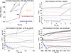 |
Fig. 1 Produced energyfor the standard scenario (top left) and superbubble kinematics for different assumptions about the energy contributors; top right (standard): winds and SNe for all massive stars and energy output from all black holes and neutron stars; bottom left (no BH acc, late SN): only SNe of starsless massive than 25 M⊙ that explode after8.79 Myr; bottom right (dark remnant acc): only sudden accretion onto the dark remnants(thick lines: black holes, only; thin lines: also neutron stars). The timescale for the global evolution of the GC is chosen at the birth of a coeval first generation of stars. The abscissae indicate the respective starting times of the three considered ejection scenarios, which corresponds to the moment when the considered energy sources become available. In scenario 3 this could happen any time once all the dark remnants have formed, i.e., after the last SN at 35 Myr after the birth of the 1G stars. Within each kinematics plot, the upper diagram shows the bubble radius (solid line) and the Rayleigh-Taylor scale (dash-dotted line), with the red dashed line indicating the half-mass radius. The middle diagram displays the shell velocity (solid line) and the escape velocity at the current bubble radius (red dashed line). The acceleration (positive: solid black line, negative: solid blue line) is shown in the lower diagram, with the gravitational acceleration at the current radius shown as a red dashed line. |
We show the energy injection together with the resulting bubble kinematics for the three respective assumptions about the energy injection law in Fig. 1. In the standard case (all energy sources active), the shell expands very slowly to about 4 Myr and in an oscillatory manner, as seen from the alternating sign of the acceleration. Once it reaches r1/2, the acceleration increases strongly and stays at a high level throughout, as expected from the above analysis. The shell reaches the local escape speed (red dashed line in the middle panels) at about 4.3 Myr, which is too late to avoid pressure loss due to the RT instability. The cluster’s gas, which is now in the shell fragments, should therefore remain bound to the cluster. For the second scenario (no BH, late SN), the shell starts to fast accelerate after about 0.5 Myr after the SN activity is assumed to start. However, the escape speed is reached only after 1.2 Myr. The shell is RT unstable long before, and therefore this scenario does not lead to gas expulsion, either. The situation is different for the third scenario, dark remnant accretion: Here, the shell reaches escape speed immediately, due to the sudden power increase. The velocity drops slightly because of the hydrodynamic evolution of the bubble. The escape speed is reached again after only 0.06 Myr and even 0.03 Myr if one includes the neutron stars. The RT instability is not able to affect the entire shell, and consequently, the gas is expelled from the cluster. We have also investigated cases with initial masses Mtot = 106 M⊙ and Mtot = 2 × 10⁷ M⊙ with very similar results. The only difference is that for the high-mass cluster, gas expulsion by dark remnant accretion only works with the help of the neutron stars. The crossing time for the model clusters  , is 0.22, 0.05, and 0.034 Myr, for the 1, 9, and 20 × 106 M⊙ clusters, respectively, using the definition of Decressin et al. (2010). For all our dark remnant accretion cases with the exception of the black-hole-only case for the high-mass cluster, the shells reach the half-mass radius much faster, and we may expect that the outer 1G stars will also be lost (compare Decressin et al. 2010). We have investigated the parameter space in ϵsf and r1/2. For both parameters, we find critical values, above which gas expulsion by SNe only, or by the power sources in our standard scenario would be possible. They are excessive, apart from perhaps the lowest mass case, where a GC may lose its gas at ϵsf > 47%. Yet, this value is too high to expell a significant number of 1G stars (Decressin et al. 2010). Similarly at ϵsf = 0.33, the SNe succeed only for r1/2 > 4 pc, which is on the high end of the observed values.
Minimum star formation efficiency and half-mass radius for SN feedback to be able to expel the gas.
3. Gas expulsion powered by dark-remnant accretion and possible observational tests
Up to now, the gas expulsion scenario via SNe has been central to the two main scenarios for self-enrichment in GCs(e.g. Baumgardt et al. 2008; D’Ercole et al. 2008; Decressin et al. 2010). Here we show that this does not generally work for simple and standard assumptions about gas expulsion via a superbubble. While the energy injected by SNe in total is sufficient, it is not delivered fast enough to overcome the RT instability. The result should not be restricted to the Plummer model: Any GC formation scenario should involve a strongly concentrated gas cloud. The gravitational pull will always be strongest on scales comparable to the half-mass radius. Sudden acceleration, when the gravitational well is overcome, and RT instability, are the natural consequences. The asymptotic acceleration is particularly strong for the Plummer model. It is likely to occur, however, albeit at a weaker level for all reasonable profiles (compare Eq. (4) and Fig. 1).
The only way to overcome the shell destruction by the RT instability is to inject the energy sufficiently fast, such that the gravitational well becomes less important for the dynamics. We show that a sudden activation of all dark remnants– a hypothesis, details of which need to be worked out in the future –is plausibly sufficient for this purpose. Here, we have adopted a general efficiency factor of 20%, mainly for consistency with previous work (Decressin et al. 2010). How may we motivate such an efficiency factor for dark remnant accretion?The Bondi accretion rate,  , M3 being the remnant mass in units of 3 M⊙, n6 the ISM number density in 106 cm-3 and v1 the higher of relative velocity and ISM sound speed in km s-1, may exceed the Eddington accretion rate by a large factor whenever the star is close to its outer turning point. Assembling mass to its vicinity in this phase, a remnant may plausibly be activated for a large part of the orbit. Accretion onto compact stellar sized objects usually leads to emission in the X-ray part of the spectrum (e.g. Chiang et al. 2010). For our standard model cluster, the hydrogen column density is about NH ≈ 1025 cm-2, i.e. it is Compton-thick and a large part of the radiated energy might be absorbed.The shells should have densities of about 106−7 cm-2 and accordingly cool down (Sutherland & Dopita 1993), collapse, remain neutral, and therefore also absorb X-rays efficiently. Additionally, there might be jets, which in the case of supermassive black holes are also known to come sometimes close to the Eddington luminosity (e.g. Krause 2005b; Celotti & Ghisellini 2008). Since the compact objects in this scenario would not accrete from a binary companion, but from the general ISM, one may speculate that the jet powers might also be comparable to the supermassive black hole case. Jets communicate their energy efficiently to their surroundings via radio lobes (e.g. Gaibler et al. 2009).For our dark-remnant accretion scenario, we find a limiting initial cloud mass of about 107 M⊙ above which the cold gas may not be ejected and therefore might form additional stars. This might contribute to explanations of the observed differences at the high-mass end of GCs (e.g. greater Fe spreads, Carretta et al. 2010).
It would be challenging to detect the dark remnants during their active phases, as the emission peaks in the X-ray part of the spectrum and the clusters should be Compton-thick at that time. The total X-ray luminosity of the cluster should be low, about 1041 erg/s, the active time from our calculations is only about 104−105 years, and the prime objects of interest are high-redshift galaxies. If the radio luminosity were similar, one would expect fluxes of about μJy, well in the reach of the upcoming Square Kilometre Array radio telescope (SKA) (e.g. Krause et al. 2009, and references therein). One could at least constrain well-defined models of cluster formation. If GC-formation was triggered by galactic scale shock waves (Harris & Harris 2011), e.g. associated with galactic winds and jets (Krause 2002, 2005a), where the GCs are supposed to form in a galactic wind shell, one might expect some active GCs during the time when the jet is active too, thus marking the relevant evolutionary epoch of the GCs. The dark-remnant driven bubbles could easily reach sizes of kpc or even 10 kpc on timescales of about 107 years. They might then leave a signature in the Faraday rotation signal if seen against a polarised background source. The SKA should also be able to detect high-redshift radio lobes in polarisation (Krause et al. 2009). The plasma closest to the radio sources is usually responsible for a big part of the rotation measure. Changing the structure of this material can leave observable features in Faraday rotation maps (Huarte-Espinosa et al. 2011).
While the 2G formation scenario in the supershell proposed in these papers did not stand up to observational scrutiny (e.g. because SN ejecta are now thought not to be mixed with the gas that forms the 2G stars), the hydrodynamics is still valid.
Acknowledgments
We thank the referee, R. McCray, for comments that helped to improve this paper. This research was supported by the cluster of excellence “Origin and Structure of the Universe” (www.universe-cluster.de) and the ESF EUROCORES Programme “Origin of the Elements and Nuclear History of the Universe” (grants 189 and 190). C.C. and T.D. also acknowledge financial support from the Swiss National Science Foundation (FNS) and the French Programme National de Physique Stellaire (PNPS) of CNRS/INSU.
References
- Bagetakos, I., Brinks, E., Walter, F., et al. 2011, AJ, 141, 23 [NASA ADS] [CrossRef] [Google Scholar]
- Baumgardt, H., Kroupa, P., & Parmentier, G. 2008, MNRAS, 384, 1231 [NASA ADS] [CrossRef] [Google Scholar]
- Bernstein, I. B., & Book, D. L. 1978, ApJ, 225, 633 [NASA ADS] [CrossRef] [Google Scholar]
- Brown, J. H., Burkert, A., & Truran, J. W. 1991, ApJ, 376, 115 [NASA ADS] [CrossRef] [Google Scholar]
- Brown, J. H., Burkert, A., & Truran, J. W. 1995, ApJ, 440, 666 [NASA ADS] [CrossRef] [Google Scholar]
- Carretta, E., Bragaglia, A., Gratton, R. G., et al. 2010, ApJ, 714, L7 [NASA ADS] [CrossRef] [Google Scholar]
- Celotti, A., & Ghisellini, G. 2008, MNRAS, 385, 283 [NASA ADS] [CrossRef] [Google Scholar]
- Chandrasekhar, S. 1961, Hydrodynamic and hydromagnetic stability (Oxford University Press) [Google Scholar]
- Charbonnel, C. 2010, in IAU Symp., 266, eds. R. de Grijs, & J. R. D. Lépine, 131 [Google Scholar]
- Chiang, C. Y., Done, C., Still, M., & Godet, O. 2010, MNRAS, 403, 1102 [NASA ADS] [CrossRef] [Google Scholar]
- Churchwell, E., Povich, M. S., Allen, D., et al. 2006, ApJ, 649, 759 [NASA ADS] [CrossRef] [Google Scholar]
- Decressin, T., Charbonnel, C., & Meynet, G. 2007a, A&A, 475, 859 [NASA ADS] [CrossRef] [EDP Sciences] [Google Scholar]
- Decressin, T., Meynet, G., Charbonnel, C., Prantzos, N., & Ekström, S. 2007b, A&A, 464, 1029 [NASA ADS] [CrossRef] [EDP Sciences] [Google Scholar]
- Decressin, T., Baumgardt, H., Charbonnel, C., & Kroupa, P. 2010, A&A, 516, A73 [NASA ADS] [CrossRef] [EDP Sciences] [Google Scholar]
- D’Ercole, A., Vesperini, E., D’Antona, F., McMillan, S. L. W., & Recchi, S. 2008, MNRAS, 391, 825 [NASA ADS] [CrossRef] [Google Scholar]
- D’Ercole, A., D’Antona, F., & Vesperini, E. 2011, MNRAS, 415, 1304 [NASA ADS] [CrossRef] [MathSciNet] [Google Scholar]
- Gaibler, V., Krause, M., & Camenzind, M. 2009, MNRAS, 400, 1785 [NASA ADS] [CrossRef] [Google Scholar]
- Gratton, R. G., Carretta, E., & Bragaglia, A. 2012, A&ARv, 20, 50 [CrossRef] [Google Scholar]
- Harris, W. E. 1996, AJ, 112, 1487 [NASA ADS] [CrossRef] [Google Scholar]
- Harris, G. L. H., & Harris, W. E. 2011, MNRAS, 410, 2347 [Google Scholar]
- Huarte-Espinosa, M., Krause, M., & Alexander, P. 2011, MNRAS, 418, 1621 [NASA ADS] [CrossRef] [Google Scholar]
- Jaskot, A. E., Strickland, D. K., Oey, M. S., Chu, Y.-H., & García-Segura, G. 2011, ApJ, 729, 28 [NASA ADS] [CrossRef] [Google Scholar]
- Krause, M. 2002, A&A, 386, L1 [NASA ADS] [CrossRef] [EDP Sciences] [Google Scholar]
- Krause, M. 2003, A&A, 398, 113 [NASA ADS] [CrossRef] [EDP Sciences] [Google Scholar]
- Krause, M. 2005a, A&A, 436, 845 [NASA ADS] [CrossRef] [EDP Sciences] [Google Scholar]
- Krause, M. 2005b, A&A, 431, 45 [NASA ADS] [CrossRef] [EDP Sciences] [Google Scholar]
- Krause, M., Alexander, P., Bolton, R., et al. 2009, MNRAS, 400, 646 [NASA ADS] [CrossRef] [Google Scholar]
- Prantzos, N., & Charbonnel, C. 2006, A&A, 458, 135 [NASA ADS] [CrossRef] [EDP Sciences] [Google Scholar]
- Prantzos, N., Charbonnel, C., & Iliadis, C. 2007, A&A, 470, 179 [NASA ADS] [CrossRef] [EDP Sciences] [Google Scholar]
- Schaerer, D., & Charbonnel, C. 2011, MNRAS, 413, 2297 [NASA ADS] [CrossRef] [MathSciNet] [Google Scholar]
- Sutherland, R. S., & Dopita, M. A. 1993, ApJS, 88, 253 [NASA ADS] [CrossRef] [Google Scholar]
- Vesperini, E., McMillan, S. L. W., D’Antona, F., & D’Ercole, A. 2010, ApJ, 718, L112 [NASA ADS] [CrossRef] [Google Scholar]
- Weaver, R., McCray, R., Castor, J., Shapiro, P., & Moore, R. 1977, ApJ, 218, 377 [NASA ADS] [CrossRef] [Google Scholar]
- Wilkinson, M. I., Hurley, J. R., Mackey, A. D., Gilmore, G. F., & Tout, C. A. 2003, MNRAS, 343, 1025 [NASA ADS] [CrossRef] [Google Scholar]
All Tables
Minimum star formation efficiency and half-mass radius for SN feedback to be able to expel the gas.
All Figures
|
Fig. 1 Produced energyfor the standard scenario (top left) and superbubble kinematics for different assumptions about the energy contributors; top right (standard): winds and SNe for all massive stars and energy output from all black holes and neutron stars; bottom left (no BH acc, late SN): only SNe of starsless massive than 25 M⊙ that explode after8.79 Myr; bottom right (dark remnant acc): only sudden accretion onto the dark remnants(thick lines: black holes, only; thin lines: also neutron stars). The timescale for the global evolution of the GC is chosen at the birth of a coeval first generation of stars. The abscissae indicate the respective starting times of the three considered ejection scenarios, which corresponds to the moment when the considered energy sources become available. In scenario 3 this could happen any time once all the dark remnants have formed, i.e., after the last SN at 35 Myr after the birth of the 1G stars. Within each kinematics plot, the upper diagram shows the bubble radius (solid line) and the Rayleigh-Taylor scale (dash-dotted line), with the red dashed line indicating the half-mass radius. The middle diagram displays the shell velocity (solid line) and the escape velocity at the current bubble radius (red dashed line). The acceleration (positive: solid black line, negative: solid blue line) is shown in the lower diagram, with the gravitational acceleration at the current radius shown as a red dashed line. |
| In the text | |
Current usage metrics show cumulative count of Article Views (full-text article views including HTML views, PDF and ePub downloads, according to the available data) and Abstracts Views on Vision4Press platform.
Data correspond to usage on the plateform after 2015. The current usage metrics is available 48-96 hours after online publication and is updated daily on week days.
Initial download of the metrics may take a while.