| Issue |
A&A
Volume 546, October 2012
|
|
|---|---|---|
| Article Number | A126 | |
| Number of page(s) | 9 | |
| Section | Galactic structure, stellar clusters and populations | |
| DOI | https://doi.org/10.1051/0004-6361/201219926 | |
| Published online | 18 October 2012 | |
Gravitational microlensing as a test of a finite-width disk model of the Galaxy
1
Institute of Physics, Jagellonian University,
Reymonta 4,
30059
Kraków,
Poland
2
Institute of Nuclear Physics, Polish Academy of Sciences,
Radzikowskego 152,
31342
Kraków,
Poland
e-mail: This email address is being protected from spambots. You need JavaScript enabled to view it.
Received:
29
June
2012
Accepted:
21
August
2012
Abstract
The aim of this work is to show, in the framework of a simple finite-width disk model, that the amount of mass seen through gravitational microlensing measurements in the region 0 < R < R° is consistent with the dynamical mass ascertained from Galaxy rotation after subtracting gas contribution. Since microlensing only detects compact objects, this result suggests that a non-baryonic mass component may be negligible in this region.
Key words: gravitational lensing: micro / Galaxy: bulge / Galaxy: disk / Galaxy: structure / dark matter
© ESO, 2012
1. Introduction
Spiral galaxies are customarily regarded as disk-like objects imbedded in a spheroidal halo of non-baryonic dark matter (NDM). In this picture the rotation of galaxies is governed mainly by the gravitational field of NDM halo, at least at larger radii.
But this scenario might not be typical, because rotation of some of spiral galaxies can be explained with a negligible (if any) amount of NDM. For these galaxies, a thin disk model approximation has proven to be quite satisfactory (Jałocha et al. 2008, 2010b). There was also a successful attempt at explaining high transverse gradients in the Galaxy rotation in the same disk model framework (Jałocha et al. 2010c), whereas including a significant spheroidal mass component proved to reduce the predicted gradient to values that are inconsistent with measurements. There is also a recent result (Moni Bidin et al. 2012) showing that the kinematics of the thick disk stars in the solar neighborhood is consistent with the visible mass alone, and there is no place for a spheroidal distribution of NDM, although the assumptions of this result are the subject of debate (Bovy & Tremaine 2012).
The above results suggest that the overall mass distribution in Galaxy might be flattened rather than spheroidal, at least in the Galaxy interior. In this case, the disk model description would be more appropriate to describing the true mass distribution in this region than mass models with a dominating spheroidal mass component. Further independent arguments that would help for deciding about the properties of mass distribution in Galaxy are necessary. To this end we apply the gravitational microlensing method as a means to determining the mass residing in compact objects, and compare the results for radii R < R° with predictions of a finite-width disk model.
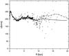 |
Fig. 1 Rotation of Galaxy. Unified rotation velocity measurements (points) (see the text for references) and two model rotation curves A (thick line) (Sofue et al. 2009) and B (dot-dashed line) (Sofue et al. 1999) used to obtain surface mass density. |
It is important that in the same region where microlensing results are known, the Galactic rotation curve is relatively well determined. Figure 1 shows rotation data for the Galaxy from various independent measurements (Burton & Gordon 1978; Clemens 1985; Fich et al. 1989; Demers & Battinelli 2007; Blitz et al. 1982; Honma & Sofue 1997), together with two model rotation curve fits obtained in Sofue et al. (2009) and Sofue et al. (1999), which we use in our calculations and refer to as A and B, respectively. They are used, because they agree well with the data points in the region of interest. Rotation curve A was obtained assuming the reference velocity Θ° = 200 km s-1. Rotation curve B assumes Θ° = 220 km s-1. Our results are based on these two curves, although in Sect. 2.3, in order to estimate the influence of the uncertainty in the determination of the parameter Θ° on our results concerning the optical depth, we also use a rotation curve from McMillan (2011) that is based on the terminal rotation curve data and a high value Θ° = 239 km s-1 preferred by the author.
The surface mass density in thin disk model can be obtained with the help of the following
integral mapping v(R) – the tangential component of Galaxy
rotation in the disk plane – to the surface mass
density σ(R) in the disk plane (representing a column
mass density): 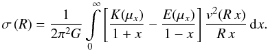 (1)Here, R is
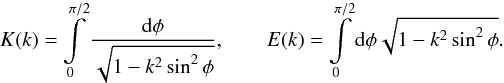
the radial variable in the disk plane, K and E are
complete elliptic integrals of the first and second kind1,
(1)Here, R is
the radial variable in the disk plane, K and E are
complete elliptic integrals of the first and second kind1,  and x is a dimensionless integration variable. Mathematical details are
given in Appendix A. In studying galaxies with the
use of the expression (1), it is assumed that
a galaxy is a flattened disk-like object rather than spheroidal and that the motion of
matter is predominantly circular. The central bulge can also be described in this model by
the appropriate substitute column mass density. One should recall that the relation between
the mass distribution and the rotation law is qualitatively different from that valid under
spherical symmetry. It is nonlocal in the sense that the total rotation field is needed to
determine the surface mass density at a given radius. Cutting off integration introduces
some error, however it is usually not significant for radii smaller than 0.6 of the cutoff
radius (Bratek et al. 2008). This condition is
satisfied in the region of our interest. The resulting surface mass densities corresponding
to rotation curves A and B are shown in Fig. 2.
and x is a dimensionless integration variable. Mathematical details are
given in Appendix A. In studying galaxies with the
use of the expression (1), it is assumed that
a galaxy is a flattened disk-like object rather than spheroidal and that the motion of
matter is predominantly circular. The central bulge can also be described in this model by
the appropriate substitute column mass density. One should recall that the relation between
the mass distribution and the rotation law is qualitatively different from that valid under
spherical symmetry. It is nonlocal in the sense that the total rotation field is needed to
determine the surface mass density at a given radius. Cutting off integration introduces
some error, however it is usually not significant for radii smaller than 0.6 of the cutoff
radius (Bratek et al. 2008). This condition is
satisfied in the region of our interest. The resulting surface mass densities corresponding
to rotation curves A and B are shown in Fig. 2.
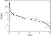 |
Fig. 2 Surface mass densities in the thin disk model corresponding to rotation curves A (solid line) and B (dot-dashed line). |
2. The microlensing method
In contrast to methods based on analyzing the Galactic rotation or the motions of halo objects, the microlensing method gives us the opportunity of measuring Galaxy mass independently of Galaxy dynamics. The method was developed and described in detail by several authors (Paczynski 1986, 1996; Schneider et al. 2006). To estimate the integrated mass distribution along various lines of sight, the method employs the phenomenon of gravitational light deflection of distant sources of light in the field of point-like masses distributed in space. A directly measured quantity in this method is the optical depth. Before going to the main analysis, let us discuss this important notion in more detail.
2.1. Optical depth along a line of sight
Suppose a point-like lens of mass M is located exactly on a line of
sight between the source of light and the observer. This line plays the role of the
optical axis. Then, the image of the source forms the Einstein ring of some angular
radius θE as perceived by the observer and concentric with
the optical axis. Let DL and DS be
the distances along the optical axis between the observer and the lens and between the
observer and the source, respectively. Expressed in terms
of θE and the gravitational deflection
angle αE, the lens equation in the weak field approximation
reduces in this particular configuration to
θE DS = αE(DS − DL).
Taking into account that  with
RE = θEDL,
we obtain
with
RE = θEDL,
we obtain  .
.
The optical depth is by definition the probability of finding a compact object (a lens)
within its Einstein radius on some plane perpendicular to the line of sight. In a given
volume element dS dDL, large enough to
contain many lenses of various masses, the corresponding probability is a sum
 over all lenses
of mass Mi,
where νi is the number density of lenses
of mass Mi. The
ratio
over all lenses
of mass Mi,
where νi is the number density of lenses
of mass Mi. The
ratio  is independent
of Mi,
and ∑ iνiMi
is simply the volume mass density of compact objects
(lenses) ρco. Integration
over DL along a given optical axis therefore gives us
is independent
of Mi,
and ∑ iνiMi
is simply the volume mass density of compact objects
(lenses) ρco. Integration
over DL along a given optical axis therefore gives us
 This
is the (integrated) optical depth along the line of sight.
This
is the (integrated) optical depth along the line of sight.
For practical reasons, the passage of a lens in front of a source of light is assumed to have occurred when the magnification of the source exceeds some threshold value. The optical depth is measured by means of counting the number of such events for millions of stars located near the Galactic center. A comprehensive description of such a measurement can be found in Moniez (2010).
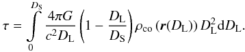
2.2. Application in the framework of a finite-width disk model
A thin disk model predicts some column density σ from Galaxy rotation
data with the help of the formula discussed earlier. To compare the disk model predictions
with the optical depth measurements, an appropriate volume mass density entering the
integral defining τ is needed. In the disk approximation,
σ can be regarded as a column mass density assigned to a volume mass
density ρ. This identification is also frequently made in modeling
galactic disks. The column mass density is defined by means of the integral
 , where R,Z are
Galacto-centric cylindrical coordinates and the axial symmetry has been assumed.
, where R,Z are
Galacto-centric cylindrical coordinates and the axial symmetry has been assumed.
The integration in τ is carried out along a line of sight joining the observer located at X⊙ = [R°,0,0] and a source located at X⊗, where X⊗ = X⊙ + (1 + χ)R°[− cosbcosl, − cosbsinl,sinb]. Here, b is the Galactic latitude, l the Galactic longitude, and (1 + χ)R° is the distance of the source of light from the Sun (χ is a dimensionless position parameter). A convenient parametric description of the line of sight is X(s) = X⊙ + s(X⊗ − X⊙) (then DL(s) = s(1 + χ)R° and DS = (1 + χ)R°). On assuming the standard exponential profile ρ(R,Z) = ρ(R,0) e − |Z|/h with a fixed scale height h, the line integral τ becomes a function of b, l and χ:
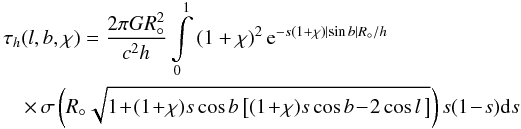 (2)where
σ is a known function.
(2)where
σ is a known function.
The observed sources of light are located in the vicinity of the Galactic center. The
measurements we use are presented as pairs (τ,b) for
various b with some errors Δτ. They are taken from
(Moniez 2010) as averages over a domain
of l around Galactic center. All of the fields used are placed within
the area presented in Fig. 14 in Hamadache et al.
(2006), although the most important region
is l ∈ (−5°,5°). The precise
value of χ is not known and its uncertainty must somehow be taken into
account in the model of τ. Either way, in a first approximation one can
assume l = 0 and χ = 0, in which case (2) reduces to
τh(0,b,0) ≈ τh(b), where
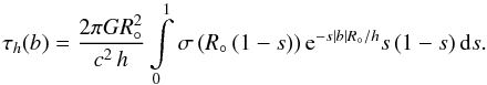 (3)In
τh(b) we used the
approximations cosb ≈ 1 and sinb ≈ b,
since |b| < 0.1 radians for the observed sources
of light.
(3)In
τh(b) we used the
approximations cosb ≈ 1 and sinb ≈ b,
since |b| < 0.1 radians for the observed sources
of light.
Before using the above integrals, a remark should be made concerning the appropriate choice for σ. We recall that the disk model gives the surface density describing the gravitating masses, regardless of their nature, whereas the microlensing events only concern compact objects. Accordingly, in making comparisons, the contribution from continuous media such as gas should be subtracted from the density.
For estimating the gas contribution we used the neutral and molecular hydrogen density profiles obtained by Misiriotis et al. (2006) from COBE/DIRBE and COBE/FIRAS observations. The column mass density of gas is then found to be approximately four third of that for hydrogen. It includes the contribution from helium. The result of this procedure is shown in Fig. 3.
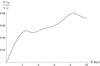 |
Fig. 3 Ratio of the hydrogen surface mass density σH relative to the total surface density accounting for the Galaxy rotation in the thin disk model. A factor 4/3 has been included to account for the helium abundance. |
The relation τh(b) is plotted in Fig. 4 for several values of b. As is seen, the predicted optical depth has a correct order of magnitude. Its dependence on the scale height is significantly weaker at higher latitudes.
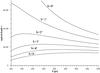 |
Fig. 4 Optical depth τh(b) in disk model as a function of the disk scale height h shown for various lines of sight, labeled by the corresponding latitudes b (in degrees). |
To find a better model of the optical depth, the uncertainty in χ in the integral (2) and an averaging procedure of the observational data over l must be simulated. To this end a Monte Carlo method can be used.
2.2.1. A Monte Carlo method
For a given value of b, a collection of lines of sight (called ensemble) is chosen randomly with some probability distribution for various pairs (l,χ), so that X⊗ is always in some region in the vicinity of the Galactic center. Then τ(l,b,χ) is calculated for every element of the ensemble, and next, the average value over the ensemble and the respective dispersion is determined. In our simulation we assumed a uniform distribution for χ and l: |χ| < 0.125 (that is, ±1 kpc), |l| < 0.017 (that is, ±1°)2. We also used an auxiliary uniform random variable Σ ∈ (0,σ(0)). At a fixed b we choose those from among the random triples (χ,l,Σ) for which Σ < σ(R). As a result, the distribution of X⊗ is weighted by σ.
2.3. The results
The frequently used value for the scale height is h = 325 pc. This standard choice is consistent with the scale height parameter for M-dwarfs of 320 ± 50 pc obtained by Gould et al. (1997).
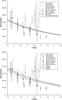 |
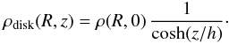
Fig. 5 Optical depths in disk model with the disk scale height h = 325 pc. Points represent the observational data averaged over longitude within the range out to l = ± 5°. Top panel: the result for the rotation curve A (thick line) and after subtracting the gas contribution (thin line). Bottom panel: comparison of optical depths for different model rotation curves: A (solid line) and B (dashed line) and, in addition, the rotation curve based on the McMillan data (dotted line) (without gas subtraction and with R° = 8.29 kpc preferred by McMillan). |
The optical depth calculated in accord with Eq. (3) is plotted in Fig. 5 for h = 325 pc and compared with the optical depths measured by several collaborations: MACHO (Popowski et al. 2005), OGLE (Sumi et al. 2006), EROS (Hamadache et al. 2006), and MOA (Sumi et al. 2003). These data were collected and discussed in a review (Moniez 2010). There is a subclass in the data consisting of bright stars. Separation of bright sources allows reducing the blending effect, which is a serious source of uncertainty in the optical depth (Alard 1997; Smith et al. 2007). It is seen that the optical depth predicted in the framework of our model fits the data quite well when the bright stars are considered. In Fig. 6 the result of the Monte Carlo procedure described earlier was shown and compared with the result shown in Fig. 5. The simulation reproduces the optical depths consistently with measurements. The Monte Carlo standard deviation also takes some information about the expected uncertainty into account in the distribution of sources around the Galactic center (as a function of longitude and distance to the source DS). It is worth noting that this uncertainty is comparable with the observational error bars. Moreover, comparing results in Fig. 5, shows that determining the optical depth hardly depends on the assumed rotation curve, suggesting indirectly that the result is not very sensitive to changes in parameter Θ° in the range from 200 km s-1 to 239 km s-1. For comparison, in addition to the rotation curves A and B, we consider the third rotation curve, which is based on the terminal rotation curve data from McMillan (2011) with the assumption of a higher value Θ° = 239 km s-1.
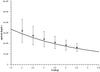 |
Fig. 6 Monte Carlo simulation of the optical depth (and standard deviation) at various latitudes b (solid circles+bars), compared with another model (discussed earlier) assuming the sources of light to be located on the symmetry axis (solid line). |
2.4. The influence of the solar Galactocentric distance R◦
In our calculations we adopted the frequently used value of the solar Galactocentric distance R° = 8.0 kpc, the same as in Avedisova (2005), where a review of other estimations can be found. In modeling microlensing in the Galaxy, other values are sometimes preferred. In the Galactic model presented by the EROS collaboration (Derue et al. 1999), the value recommended by the IAU R° = 8.5 kpc is used. Because the integrand in the formula defining the optical depth (3) is small near the Sun’s position, the choice of R° cannot alter the results significantly, however. When R° is increased from R° = 8.0 kpc to R° = 8.5 kpc in the integral (3), there is a corresponding change in the optical depth of Δτ = +0.1 × 10⁻⁶ at b = 1° and only Δτ = −0.04 × 10⁻⁶ at b = 5°. One can also find a lower value for R° of 7.62 kpc (Eisenhauer et al. 2005). Replacing R° = 8.0 kpc with R° = 7.62 kpc in the integral (3) gives rise to a change in the optical depth of Δτ = −0.1 × 10⁻⁶ at b = 1° and only Δτ = +0.02 × 10⁻⁶ at b = 5°. This shows that the optical depth is not sensitive to the changes in the estimate of R° within the limits most frequently met in the literature.
2.5. The influence of the bulge structure
The disk model predicts a substitute surface density σ(R) in the disk plane that accounts for the rotation curve. It can be regarded as the column mass density. If the true mass distribution is flattened then the description in terms of the column mass density should be sufficient for a dynamical model, but an appropriate volume mass reconstruction is needed when studying the microlensing. In the previous section we assumed that the vertical profile of the total volume mass density ρ(R,z) changed exponentially: ρ(R,z) = ρ(R,0) e−|z|/h = σ(R) e−|z|/h/2h. In particular, the central bulge can be described in terms of its own column mass density, which contributes to the total mass density. But the observations of the bulge (for example, Binney et al. 1997; Bissantz & Gerhard 2002) indicate that a spherically symmetric distribution of matter or even a three-axial ellipsoid would better approximate the central part of the Galaxy, and close to the center there can be some correction to the density profile we use. The stars residing in the central bulge contribute significantly to the optical depth, thus the particular geometry of mass distribution may have some effect on the accuracy of our result. Therefore, some estimation of the uncertainty is indispensable in our predictions concerning the optical depth.
To this end, we replace the central part extending out to 1 kpc by a spherically symmetric bulge and check how this change in the mass distribution alters the optical depth. Since the dynamical mass inside 1 kpc is comparable in both models (the disk model gives M1 kpc = 1.061 × 10¹⁰ M⊙, whereas for the spherical bulge M1 kpc = 1.137 × 10¹⁰ M⊙), we do not expect large discrepancies in their predictions. A possible change by a factor of order of unity may result from a change in the iso-density surfaces and from a small change in mass distribution outside 1 kpc compensating for any excess from the rotation that including a spherically symmetric part may have caused in the gravitational potential.
With the bulge included, the integral for the optical depth splits as follows
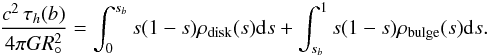 The
first term is the contribution from the thick disk, and the second term is the
contribution from the central bulge, where ρbulge
and ρdisk are understood as functions
of R(s) and z(s)
along the lines of sight. The integration limits are determined by the bulge size
Rb = (1 − sb)R° = 1 kpc.
The density ρbulge at the spherical radius
The
first term is the contribution from the thick disk, and the second term is the
contribution from the central bulge, where ρbulge
and ρdisk are understood as functions
of R(s) and z(s)
along the lines of sight. The integration limits are determined by the bulge size
Rb = (1 − sb)R° = 1 kpc.
The density ρbulge at the spherical radius
 can be found from the mass function M(r) of the bulge
 and
this M(r) in turn contributes to the rotation curve. We
assume that the bulge accounts for the measured rotation curve for radii
R < Rb.
In this case we have
M(r) = r v2(r)/G,
while for
R > Rb
we assume the contribution from the bulge to be
Keplerian:
and
this M(r) in turn contributes to the rotation curve. We
assume that the bulge accounts for the measured rotation curve for radii
R < Rb.
In this case we have
M(r) = r v2(r)/G,
while for
R > Rb
we assume the contribution from the bulge to be
Keplerian:  .
As previously, for small b’s the disk volume density is
ρdisk = σ1(R°(1 − s)) e−s|b|R°/h/2h,
where σ1 accounts for the remaining part of
rotation
.
As previously, for small b’s the disk volume density is
ρdisk = σ1(R°(1 − s)) e−s|b|R°/h/2h,
where σ1 accounts for the remaining part of
rotation  not explained by the bulge (a
similar decomposition of rotation was applied to another galaxy in Jałocha et al. 2010a). The decomposition of the rotation curve is
plotted in Fig. 7. The required surface
density σ1(R) corresponding
to v1(R) can be found by applying the
iteration method described in Jałocha et al.
(2008). The resulting optical depth is plotted in Fig. 8. As expected, the correction from the presence of the bulge is so
small (of the order of Δτ = 0.2 × 10⁻⁶) that it cannot
change the main conclusion of the previous paragraph.
not explained by the bulge (a
similar decomposition of rotation was applied to another galaxy in Jałocha et al. 2010a). The decomposition of the rotation curve is
plotted in Fig. 7. The required surface
density σ1(R) corresponding
to v1(R) can be found by applying the
iteration method described in Jałocha et al.
(2008). The resulting optical depth is plotted in Fig. 8. As expected, the correction from the presence of the bulge is so
small (of the order of Δτ = 0.2 × 10⁻⁶) that it cannot
change the main conclusion of the previous paragraph.
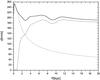 |
Fig. 7 Decomposition of the measured rotation curve into a bulge and a disk contribution. |
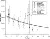 |
Fig. 8 Optical depth in a model with a spherically symmetric bulge (thin dashed line) and the disk model prediction (solid line). |
2.6. Influence of the vertical structure
The disk model predicts only the column mass
density σ(R), and its reprojection to a volume mass
density ρ(R,z) depends on the additional assumption
about the adopted density fall-off in the vertical direction. It is therefore
indispensable to estimate the influence of this assumption on the predicted optical depth.
As the starting point, we adopt a single exponential vertical fall-off
ρ(R,z) = ρ(R,0) e−|z|/h
with the scale height parameter h = 325 pc. The dependence on the scale
height parameter has been already checked and presented in Fig. 4. It shows that when the effective change of the scale height is not
large, the results cannot be changed significantly, especially for the higher latitudes.
In this section, we compare our result with the ones for two other vertical distributions
of matter. First, we consider a double exponential vertical profile:
 The
parameters h1 = 320 pc for the thinner disk,
h2 = 643 pc for the thicker disk, and the fraction
β = 0.216 are taken from Gould et al.
(1997). Likewise, we also consider the hyperbolic cosine profile
used in van Altena et al. (2004):
The
parameters h1 = 320 pc for the thinner disk,
h2 = 643 pc for the thicker disk, and the fraction
β = 0.216 are taken from Gould et al.
(1997). Likewise, we also consider the hyperbolic cosine profile
used in van Altena et al. (2004):
 As
we show in Sect. 2.9, this profile approximates the
observations better in the solar neighborhood and improves the mass-to-light ratio. The
comparison of the model curves τ(b) for the disk
vertical density distribution profiles mentioned above is presented in Fig. 9. The calculations are made after subtracting the gas
contribution and by considering the spherical bulge component. As we expected, the choice
of the particular vertical density fall-off could only slightly change the results.
Replacement of a single exponential profile by a double exponential profile reduces the
optical depth approximately by Δτ = 0.2 × 10⁻⁶.
As
we show in Sect. 2.9, this profile approximates the
observations better in the solar neighborhood and improves the mass-to-light ratio. The
comparison of the model curves τ(b) for the disk
vertical density distribution profiles mentioned above is presented in Fig. 9. The calculations are made after subtracting the gas
contribution and by considering the spherical bulge component. As we expected, the choice
of the particular vertical density fall-off could only slightly change the results.
Replacement of a single exponential profile by a double exponential profile reduces the
optical depth approximately by Δτ = 0.2 × 10⁻⁶.
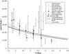 |
Fig. 9 Optical depth calculated after subtracting the gas contribution, with the inclusion of the spherical bulge, shown for all of the vertical density distributions considered in the text. The thin dotted line represents the reference model – a disk with the exponential vertical profile with the scale height h = 325 pc. The thick dotted line corresponds to the disk with a double exponential vertical profile, and the solid line represents the hyperbolic cosine vertical profile. |
Finally, we discuss a more complicated situation. The case of a three-axial ellipsoid is beyond the scope of the simple axi-symmetric dynamical model of the Galaxy, nevertheless, a correction to the optical depth connected with the presence of the bar should be within an order of magnitude as in the case of the spherically symmetric bulge considered earlier. We have seen above that our result is very stable against small changes in the mass distribution. Similarly, considering a bar-like structure would only introduce higher multipoles to the mass distribution that should not affect qualitatively our main conclusion. In the next section we study this issue in a more detail.
2.7. Model uncertainties and the bar issue
It is plausible that very particular assumptions about the dynamical model of the Galaxy could affect the resulting optical depth. If the model is based on the rotation curve, in preparation of which the axial symmetry is assumed, it is natural to assume axisymmetry for the distribution of the sources of light. This symmetry is consistent with the disk symmetry and with the spherical symmetry, whereas it is not consistent with the three-axial symmetry of a bar-like structure. Because of this, an axisymmetric model is not adequate for estimating the optical depth in a single, particular direction. That is why we are using a τ(b) observable, which has the meaning of the optical depth over slices of fixed longitude with latitudes around a particular b. Taking the statistical character of τ(b) into account, we performed a Monte Carlo simulation that mimics the observational situation of detecting microlensing events from many sources with various longitudes and various distances to the observer. Although the longitude of each field is well determined, the distance to the particular source of light (described by the χ parameter) is practically unknown. We have chosen a sample of pairs (l,χ) for which we used a probability distribution weighted by the surface mass density σ. The result for the τ(b) calculated for this sample is depicted in Fig. 6. It shows that on average the approximation for which the sources are located on the symmetry axis works quite well.
One of the advantages of the Monte Carlo approach is that it enables one to estimate a
possible change or uncertainty in the determination of τ that could be
introduced by deformations of the central part, in particular those due to the presence of
the bar. As previously, we do not expect changes in the main conclusion. This remark is
suggested by the fact that the dependence of the optical depth on the
longitude τ(l) (within latitudinal slices of
longitudes from around a particular l) is much weaker than the dependence
on the latitude τ(b). According to Hamadache et al. (2006), the optical depth changes by about
Δτ = 1.3 × 10⁻⁶ in the range
l ∈ (−5°,5°) while the optical
depth change in the considered range of latitudes is about
Δτ = 2.7 × 10⁻⁶. Our disk model predicts the change in the
optical depth in the range
l ∈ (−5°,5°) of about
Δτ = 1.8 × 10⁻⁶. Then, the correction connected with the
inclusion of the bar should be less than Δτ = 0.5 × 10⁻⁶.
To estimate the influence of the bar on our results, we employ the three-axial G2 model
developed in Dwek et al. (1995). It gives a volume
emissivity of the sources of light in the Galactic center: ![Mathematical equation: \begin{equation} \eta(x',y',z')=\eta_0\,{\rm exp}\left[-\frac{1}{2}\sqrt{\left[\left(\frac{x'}{x_{0}}\right)^2+\left(\frac{y'}{y_{0}}\right)^2 \right]^2+\frac{z'^4}{z_{0}{}^4}}\right]\cdot \label{emissivity} \end{equation}](/articles/aa/full_html/2012/10/aa19926-12/aa19926-12-eq138.png) (4)In Sect. 2.2 we used the following notation for the cartesian
coordinates of the source
X⊗ = [x,y,z] = R° [1 − (1 + χ)cosbcosl, − (1 + χ)cosbsinl , (1 + χ)sinb] ,
which differs from the naming convention used in Dwek
et al. (1995). If we denote by x′,
y′, z′ as the cartesian
coordinates of their coordinate system, then the appropriate transformation reads
as x′ → y,
y′ → − x,
and z′ → z.
(4)In Sect. 2.2 we used the following notation for the cartesian
coordinates of the source
X⊗ = [x,y,z] = R° [1 − (1 + χ)cosbcosl, − (1 + χ)cosbsinl , (1 + χ)sinb] ,
which differs from the naming convention used in Dwek
et al. (1995). If we denote by x′,
y′, z′ as the cartesian
coordinates of their coordinate system, then the appropriate transformation reads
as x′ → y,
y′ → − x,
and z′ → z.
We applied the formula (4) to perform our Monte Carlo simulation in which the sources of light are chosen randomly with the probability distribution proportional to the volume emissivity. This imitates the situation in which the sources are distributed within the three-axial bar. We take the parameters x0 = 2.01 kpc, y0 = 0.62 kpc, and z0 = 0.44 kpc fitted in the 3,5 μm band, although the values obtained in other bands give roughly the same result. In Fig. 10 below, we present the comparison of the Monte Carlo simulations assuming the axial symmetry and one that considers the G2 three-axial model. For this three-axial model, an extended range for longitudes is assumed |l| < 0.085 (that is, ±5°), which covers all the fields used in the preparation of data (see Fig. 14 in Hamadache et al. 2006). In the central part of the bulge (say, ±1° in the longitude), there is practically no difference between the predictions of the three-axial model and the spherically symmetric bulge models. One can see that the results for the sources distributed within the three-axial bulge are also consistent with the main disk model prediction. The correction due to the bar, combined with the dependence on the choice of the field range, gives no more than Δτ = 0.4 × 10⁻⁶. We neglect that the non-axisymmetric component affects the dynamics of the inner part of the Galaxy a bit. However, this correction also cannot be large, because the photometrically determined bulge mass in the G2 model MG2 = 1.3 × 10¹⁰ M⊙ (Dwek et al. 1995) is comparable to our estimation M1 kpc = 1.137 × 10¹⁰ M⊙.
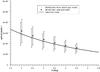 |
Fig. 10 Monte Carlo simulation of the optical depth (and the standard deviation) in the axisymmetric case (solid circles and bars) and in the presence of a three-axial bar (open circles and bars). The solid line represents the model curve based on the integral (2), in which case the sources of light lie on the symmetry axis. |
2.8. The hidden mass estimation
To estimate the amount of the hidden mass we must take the
τ(b) prediction in the thin disk model framework into
account after subtraction of the gas contribution, using rotation curve B (which gives a
more massive disk than rotation curve A), considering the spherical bulge component and
the disk double-exponential vertical fall-off. The result can be parameterized as
follows: τ(b) = c1exp(−c2|b|) × 10-6
with coefficients c1 = 4.23 ± 0.65 and
c2 = 0.228 ± 0.056. Not only the neutral and molecular
hydrogen and helium, but also other components of the total dynamical mass inside the
solar orbit of
Mtot = 6.17 × 10¹⁰ M⊙
contribute to this result. A fraction of Mtot could consist of
matter that is neither in the form of compact objects nor in the form of hydrogen and
helium clouds, which have already been subtracted. Because it would not contribute to the
measured optical depth, we call it the hidden mass. It overestimates the model optical
depth τ(b) by a
factor τhidden(b), which can be obtained by
inserting the volume mass density of the hidden
mass ρhidden(R,z) into the integral (2). Unfortunately, the
ρhidden(R,z) profile is not known. Since
this profile appears in the integrand of the relevant formula, there are various possible
profiles of ρhidden(R,z) that could lead to
the optical depth correction τhidden(b)
giving τ(b) − τhidden(b)
as the best fit to the observational optical-depth data points. For the simplicity of the
estimation, we may assume that the hidden mass density is a constant fraction of the
dynamical mass density (without gas)
ρhidden(R,z) = f ρ(R,z).
Then, the correction factor is
τhidden(b) = f τ(b),
and the observed optical depth is expected to
be (1 − f)τ(b). We find the
fraction f by fitting the formula
(1 − f) c1exp(−c2|b|) × 10-6
to the bright stars τ observations, by means of the least squares method
weighted by the observational uncertainties. The results of the fitting procedure are
depicted in Fig. 11. Taking the OGLE, MACHO, and
EROS data into account, we obtain f = −0.139 ± 0.059. Because this
fraction is negative, that would mean that an additional dynamical mass of about
|f Mtot| = (0.86 ± 0.36) ×
1010 M⊙ is needed. The data points collected
by the OGLE collaboration lie above the points collected by other groups and have a bit
larger uncertainties. If we restricted the analysis to the MACHO and EROS data, we would
get f = 0.018 ± 0.067, which translates to
|f Mtot| = (0.11 ± 0.41) ×
1010 M⊙ of the hidden mass. One should regard
all this as rough estimates. The two fits that we present are only used to find the
expectation value of the optical
depth E [τ(b)] by means of the
least squares method. On the other hand, we know what the expected variance of the optical
depth predicted by the thin disk model is, because we have performed the Monte Carlo
simulation, which gives us the
uncertainties ΔτMonte Carlo(b). They
could differ from the fit residuals. The variance assigned to our model should be
var [τ(b)] = (ΔτMonte Carlo(b))2.
Instead of checking the goodness of the fit, one can compare the model
distribution { E [τ(b)] ,var [τ(b)] }
with the observational one  .
The average
.
The average  can be taken within some narrow band in the latitude b ± 0.2 deg, and
the σ(b) is the observational uncertainty within the
band. To check the statistical hypothesis that these two distributions have the same
expectation values
can be taken within some narrow band in the latitude b ± 0.2 deg, and
the σ(b) is the observational uncertainty within the
band. To check the statistical hypothesis that these two distributions have the same
expectation values ![Mathematical equation: \hbox{$E[\tau(b)]=\bar{\tau}(b)$}](/articles/aa/full_html/2012/10/aa19926-12/aa19926-12-eq186.png) ,
one should compute the quantity:
,
one should compute the quantity: ![Mathematical equation: \begin{eqnarray*} z_b=\frac{E[\tau(b)]-\bar{\tau}(b)}{\sqrt{\frac{{\rm var}[\tau(b)]}{n}+ \frac{\sigma^2(b)}{n_b}}}\cdot \end{eqnarray*}](/articles/aa/full_html/2012/10/aa19926-12/aa19926-12-eq187.png) Here
n = 10 000 denotes the number of points generated in the Monte Carlo
simulation for the fixed latitude b,
and nb is the number of the observational
points within the band b ± 0.2 deg. The
variable zb has the normal
distribution N(0,1). Below, in Tables 1 and 2,
the appropriate values are listed in the case without the OGLE data and in the case in
which all the data are considered.
Here
n = 10 000 denotes the number of points generated in the Monte Carlo
simulation for the fixed latitude b,
and nb is the number of the observational
points within the band b ± 0.2 deg. The
variable zb has the normal
distribution N(0,1). Below, in Tables 1 and 2,
the appropriate values are listed in the case without the OGLE data and in the case in
which all the data are considered.
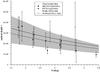 |
Fig. 11 (1 − f) c1exp(−c2|b|) × 10-6 fit to the OGLE, MACHO, and EROS bright stars optical depth data (solid line) and a similar fit to the narrowed data of MACHO and EROS bright stars data (dashed line). The filled area corresponds to the standard deviation range of the Monte Carlo simulation (including bar) described in the previous section. The c1exp(−c2|b|) × 10-6 curve is not plotted for clarity. |
Expectation value, variance, and test statistics zb in the case without OGLE data points.
Expectation value, variance, and test statistics zb in the case where all data are considered.
In both cases the test statistics zb have
values relatively close to zero. On a reasonable confidence level of
p = 0.01 one cannot reject the null hypothesis that the model
distribution { E [τ(b)] ,var [τ(b)] }
and the observational distribution
have the same expectation values. By taking the highest value
zb = 1.3, one could reject this
hypothesis on the confidence level p = 0.19; however, this would lead to
a very high probability p = 0.19 of the statistical error of the first
kind (of the rejection of the true null hypothesis). With a smaller
number n, the agreement is even better (because for
n = 10 000 the
term var [τ(b)] /n
can be neglected).
In other words, almost all observational data lie close to the expectation value E [τ(b)] , within the ±ΔMonte Carlo(b) range, which is depicted in Fig. 11. Since the fits we have obtained are close to the value f = 0, and the observational data are consistent with the Monte Carlo simulation, we are led to the conclusion that all of the dynamical mass corresponding to the rotation curve in the disk model (and after subtraction of gas) is consistent with the optical depth. The amount of the hidden mass or an additional dynamical mass that could be needed to account for the optical depth observation, is negligible in the 0 < R < R° region.
2.9. The mass-to-light ratio in the solar neighborhood in the disk model
As a cross-check for the dynamical model of the Galaxy one can ask about its prediction of the light-to-mass ratio in the solar neighborhood. To determine the profile of the local mass-to-light ratio one needs a brightness profile. It is difficult to determine the brightness profile for Galaxy in the form of a single curve. There were only attempts to determine the overall brightness in the solar vicinity by direct counting of nearby stars. Such brightness estimate in our neighborhood is quite accurate (but questionable as globally representative for the Galaxy at the same radial distance). In Flynn et al. (2006) the local I-band brightness is 29.54 L⊙/pc2. It is determined based on star counts out to 200 pc above the Galactic midplane. In the same volume there is 13.2 M⊙/pc2 of hydrogen (HI + HII + H2). Given these data, we obtain 110 M⊙/pc2 or 140 M⊙/pc2 in the disk model for the column mass density corresponding to rotation curves A or B, respectively. Subtracting four thirds of hydrogen (thus including He from the bariogenesis), because the gas is nonluminous in this band, we obtain M/LI = 3.13 or M/LI = 4.14, respectively, in the solar vicinity. Although overestimated, these values are low (and could be still reduced by including more distant objects, above z = 200 pc, which have not been included in the counting).
For a better estimate of the mass-to-light ratio in the solar neighborhood we can test other models of distribution of stars above the midplane. In van Altena et al. (2004), the profile ansatz 1/cosh(z/h) was assumed as approximating the observations better than the usual exponential falloff. Assuming our total (column) surface density of 110 M⊙/pc2 and h = 330 pc we obtain ρ = 0.11 M⊙/pc3 in the solar vicinity, so that the integrated density out to h = 200 pc gives 42 M⊙/pc2 and the corresponding M/LI = 0.83 or M/LI = 1.1 for rotation curves A or B, respectively. With exponential vertical falloff e−|z|/h (with h = 350 pc), we would have M/LI = 0.95 or M/LI = 1.47 for rotation curves A or B, respectively. These are quite reasonable and low local mass-to-light ratios, which seem to be compatible with the recent findings from the star kinematics in the solar neighborhood (Moni Bidin et al. 2012).
3. Summary and conclusions
The microlensing method determines the optical depth observable. The observable can be modeled provided the volume mass density of compact objects is known. We assumed that the total volume mass density has an exponential vertical falloff and that the associated column mass density accounts for the tangential component of rotation in the thin disk model approximation. The structure of the central bulge and the presence of the bulge do not alter the results significantly, so our results are also insensitive to slight changes in the rotation curves such as the choice of the parameter Θ. Having subtracted the gas contribution from the volume mass density obtained in this way, we modeled the optical depth and then compared the model with the optical depth measurements. It follows from the analysis that the amount of mass seen through gravitational microlensing in the region 0 < R < R° is consistent with our mass model. So that our model of the optical depth conform more to realistic measurements, we carried out a Monte Carlo simulation. It proved to mimic the measurements quite satisfactorily, since on the reasonable confidence level one could not reject the hypothesis that its expectation value equaled the expectation value of the observational data. We estimated the limits for the amount of nonbaryonic dark matter in our model inside radius R° to be (0.11 ± 0.4) × 1010 M⊙. Since microlensing only detects compact objects, the result suggests that the nonbaryonic mass component may be negligible in this region because the mass of gas and that of compact objects seen through microlensing suffice to account for Galaxy rotation in this region.
Since there are two conventions for the argument of elliptic integrals met in the literature, we give the definitions which we use (Gradshtein et al. 2007):
In the simulation that also takes the bar into account, the full range l = ±5° is considered (see Sect. 2.7).
The gravitational potential due to axisymmetric thin disk with surface mass density σ in cylindrical coordinates is
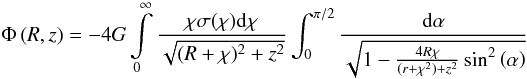
and the definition of elliptic function K can be used. Differentiation with respect to R and taking the limit z → 0 (the velocity on circular orbits in the disk plane is v2(R) = R ∂RΦ(R,0)) gives the desired result.
References
- Alard, C. 1997, A&A, 321, 424 [NASA ADS] [Google Scholar]
- Avedisova, V. S. 2005, Astron. Rep., 49, 435 [NASA ADS] [CrossRef] [Google Scholar]
- Binney, J., Gerhard, O., & Spergel, D. 1997, MNRAS, 288, 365 [NASA ADS] [CrossRef] [Google Scholar]
- Bissantz, N., & Gerhard, O. 2002, MNRAS, 330, 591 [NASA ADS] [CrossRef] [Google Scholar]
- Blitz, L., Fich, M., & Stark, A. A. 1982, ApJS, 49, 183 [NASA ADS] [CrossRef] [Google Scholar]
- Bovy, J., & Tremaine, S. 2012, ApJ, 756, 89 [Google Scholar]
- Bratek, Ł., Jałocha, J., & Kutschera, M. 2008, MNRAS, 391, 1373 [NASA ADS] [CrossRef] [Google Scholar]
- Burton, W. B., & Gordon, M. A. 1978, A&A, 63, 7 [NASA ADS] [Google Scholar]
- Clemens, D. P. 1985, ApJ, 295, 422 [NASA ADS] [CrossRef] [Google Scholar]
- Demers, S., & Battinelli, P. 2007, A&A, 473, 143 [NASA ADS] [CrossRef] [EDP Sciences] [Google Scholar]
- Derue, F., Afonso, C., Alard, C., et al. 1999, A&A, 351, 87 [NASA ADS] [Google Scholar]
- Dwek, E., Arendt, R. G., Hauser, M. G., et al. 1995, ApJ, 445, 716 [CrossRef] [Google Scholar]
- Eisenhauer, F., Genzel, R., Alexander, T., et al. 2005, ApJ, 628, 246 [NASA ADS] [CrossRef] [Google Scholar]
- Fich, M., Blitz, L., & Stark, A. A. 1989, ApJ, 342, 272 [NASA ADS] [CrossRef] [Google Scholar]
- Flynn, C., Holmberg, J., Portinari, L., Fuchs, B., & Jahreiß, H. 2006, MNRAS, 372, 1149 [NASA ADS] [CrossRef] [MathSciNet] [Google Scholar]
- Gould, A., Bahcall, J. N., & Flynn, C. 1997, ApJ, 482, 913 [NASA ADS] [CrossRef] [Google Scholar]
- Gradshtein, I., Ryzhik, I., Jeffrey, A., & Zwillinger, D. 2007, Table of integrals, series and products (Academic Press) [Google Scholar]
- Hamadache, C., Le Guillou, L., Tisserand, P., et al. 2006, A&A, 454, 185 [NASA ADS] [CrossRef] [EDP Sciences] [Google Scholar]
- Honma, M., & Sofue, Y. 1997, PASJ, 49, 453 [NASA ADS] [CrossRef] [Google Scholar]
- Jałocha, J., Bratek, Ł., & Kutschera, M. 2008, ApJ, 679, 373 [NASA ADS] [CrossRef] [Google Scholar]
- Jałocha, J., Bratek, Ł., & Kutschera, M. 2010a, Acta Phys. Pol. B, 41, 1383 [Google Scholar]
- Jałocha, J., Bratek, Ł., Kutschera, M., & Skindzier, P. 2010b, MNRAS, 406, 2805 [NASA ADS] [CrossRef] [Google Scholar]
- Jałocha, J., Bratek, Ł., Kutschera, M., & Skindzier, P. 2010c, MNRAS, 407, 1689 [NASA ADS] [CrossRef] [Google Scholar]
- McMillan, P. J. 2011, MNRAS, 414, 2446 [NASA ADS] [CrossRef] [Google Scholar]
- Misiriotis, A., Xilouris, E. M., Papamastorakis, J., Boumis, P., & Goudis, C. D. 2006, A&A, 459, 113 [NASA ADS] [CrossRef] [EDP Sciences] [Google Scholar]
- Moni Bidin, C., Carraro, G., Mendez, R. A., & Smith, R. 2012, ApJ, 751, 30 [NASA ADS] [CrossRef] [Google Scholar]
- Moniez, M. 2010, Gen. Relat. Gravit., 42, 2047 [CrossRef] [Google Scholar]
- Paczynski, B. 1986, ApJ, 304, 1 [NASA ADS] [CrossRef] [Google Scholar]
- Paczynski, B. 1996, ARA&A, 34, 419 [NASA ADS] [CrossRef] [Google Scholar]
- Popowski, P., Griest, K., Thomas, C. L., et al. (MACHO Collaboration) 2005, ApJ, 631, 879 [NASA ADS] [CrossRef] [Google Scholar]
- Schneider, P., Kochanek, C., & Wambsganss, J. 2006, Gravitational lensing: strong, weak and micro, Saas-Fee Advanced Course: Swiss Society for Astrophysics and Astronomy (Springer) [Google Scholar]
- Smith, M. C., Woźniak, P., Mao, S., & Sumi, T. 2007, MNRAS, 380, 805 [NASA ADS] [CrossRef] [Google Scholar]
- Sofue, Y., Tutui, Y., Honma, M., et al. 1999, ApJ, 523, 136 [NASA ADS] [CrossRef] [Google Scholar]
- Sofue, Y., Honma, M., & Omodaka, T. 2009, PASJ, 61, 227 [NASA ADS] [Google Scholar]
- Sumi, T., Abe, F., Bond, I. A., et al. 2003, ApJ, 591, 204 [NASA ADS] [CrossRef] [Google Scholar]
- Sumi, T., Woźniak, P. R., Udalski, A., et al. 2006, ApJ, 636, 240 [CrossRef] [Google Scholar]
- van Altena, W. F., Korchagin, V. I., Girard, T. M., Dinescu, D. I., & Borkova, T. V. 2004, in Dark Matter in Galaxies, eds. S. Ryder, D. Pisano, M. Walker, & K. Freeman, IAU Symp., 220, 201 [Google Scholar]
Appendix A: The integral transforms appearing in the disk model
The relation (1) used in the text can be
obtained from an equivalent integral expression derived in (Bratek et al. 2008) ![Mathematical equation: \appendix \setcounter{section}{1} \begin{eqnarray*} \sigma(R)= \frac{1}{\pi^2G} \left[\int\limits_0^R v^2(\chi)\biggl(\frac{K\br{{\chi}/{R}}}{ R\ \chi}-\frac{R}{\chi} \frac{E\br{{\chi}/{R}}}{R^2-\chi^2}\biggr)\ud{\chi} \cdots\right. \\ \left. \cdots+\int\limits_R^{\infty}v^2(\chi) \frac{E\br{{R}/{\chi}} }{\chi^2-R^2}\,\ud{\chi}\right]. \end{eqnarray*}](/articles/aa/full_html/2012/10/aa19926-12/aa19926-12-eq278.png) To
this end one can use the identities
To
this end one can use the identities  and
and
 with
with  ,
applied separately for χ < R
(with k = χ/R) and
for R < χ
(with k = R/χ).
The inverse relation mapping the surface density to the rotation law can be found directly
from the definition of the gravitational potential, without the usual intermediate step
through Henkel transforms (note the sign difference in (1))
,
applied separately for χ < R
(with k = χ/R) and
for R < χ
(with k = R/χ).
The inverse relation mapping the surface density to the rotation law can be found directly
from the definition of the gravitational potential, without the usual intermediate step
through Henkel transforms (note the sign difference in (1))  (A.1)The two
integrals (1) and (A.1) are quite symmetric, the inversion
transform x → 1/x
leaving μx invariant links the integral
kernels of the two integrals. We see that two physical quantities, the disk surface
density σ(R) and the centrifugal acceleration on a
circular orbit
(A.1)The two
integrals (1) and (A.1) are quite symmetric, the inversion
transform x → 1/x
leaving μx invariant links the integral
kernels of the two integrals. We see that two physical quantities, the disk surface
density σ(R) and the centrifugal acceleration on a
circular orbit  in the
disk plane, are integral transforms of each other. It would be interesting to investigate
this striking property of the disk model in more detail in the context of the theory of
integral transforms.
in the
disk plane, are integral transforms of each other. It would be interesting to investigate
this striking property of the disk model in more detail in the context of the theory of
integral transforms.
All Tables
Expectation value, variance, and test statistics zb in the case without OGLE data points.
Expectation value, variance, and test statistics zb in the case where all data are considered.
All Figures
|
Fig. 1 Rotation of Galaxy. Unified rotation velocity measurements (points) (see the text for references) and two model rotation curves A (thick line) (Sofue et al. 2009) and B (dot-dashed line) (Sofue et al. 1999) used to obtain surface mass density. |
| In the text | |
|
Fig. 2 Surface mass densities in the thin disk model corresponding to rotation curves A (solid line) and B (dot-dashed line). |
| In the text | |
|
Fig. 3 Ratio of the hydrogen surface mass density σH relative to the total surface density accounting for the Galaxy rotation in the thin disk model. A factor 4/3 has been included to account for the helium abundance. |
| In the text | |
|
Fig. 4 Optical depth τh(b) in disk model as a function of the disk scale height h shown for various lines of sight, labeled by the corresponding latitudes b (in degrees). |
| In the text | |
|
Fig. 5 Optical depths in disk model with the disk scale height h = 325 pc. Points represent the observational data averaged over longitude within the range out to l = ± 5°. Top panel: the result for the rotation curve A (thick line) and after subtracting the gas contribution (thin line). Bottom panel: comparison of optical depths for different model rotation curves: A (solid line) and B (dashed line) and, in addition, the rotation curve based on the McMillan data (dotted line) (without gas subtraction and with R° = 8.29 kpc preferred by McMillan). |
| In the text | |
|
Fig. 6 Monte Carlo simulation of the optical depth (and standard deviation) at various latitudes b (solid circles+bars), compared with another model (discussed earlier) assuming the sources of light to be located on the symmetry axis (solid line). |
| In the text | |
|
Fig. 7 Decomposition of the measured rotation curve into a bulge and a disk contribution. |
| In the text | |
|
Fig. 8 Optical depth in a model with a spherically symmetric bulge (thin dashed line) and the disk model prediction (solid line). |
| In the text | |
|
Fig. 9 Optical depth calculated after subtracting the gas contribution, with the inclusion of the spherical bulge, shown for all of the vertical density distributions considered in the text. The thin dotted line represents the reference model – a disk with the exponential vertical profile with the scale height h = 325 pc. The thick dotted line corresponds to the disk with a double exponential vertical profile, and the solid line represents the hyperbolic cosine vertical profile. |
| In the text | |
|
Fig. 10 Monte Carlo simulation of the optical depth (and the standard deviation) in the axisymmetric case (solid circles and bars) and in the presence of a three-axial bar (open circles and bars). The solid line represents the model curve based on the integral (2), in which case the sources of light lie on the symmetry axis. |
| In the text | |
|
Fig. 11 (1 − f) c1exp(−c2|b|) × 10-6 fit to the OGLE, MACHO, and EROS bright stars optical depth data (solid line) and a similar fit to the narrowed data of MACHO and EROS bright stars data (dashed line). The filled area corresponds to the standard deviation range of the Monte Carlo simulation (including bar) described in the previous section. The c1exp(−c2|b|) × 10-6 curve is not plotted for clarity. |
| In the text | |
Current usage metrics show cumulative count of Article Views (full-text article views including HTML views, PDF and ePub downloads, according to the available data) and Abstracts Views on Vision4Press platform.
Data correspond to usage on the plateform after 2015. The current usage metrics is available 48-96 hours after online publication and is updated daily on week days.
Initial download of the metrics may take a while.