| Issue |
A&A
Volume 546, October 2012
|
|
|---|---|---|
| Article Number | A14 | |
| Number of page(s) | 7 | |
| Section | Stellar atmospheres | |
| DOI | https://doi.org/10.1051/0004-6361/201219849 | |
| Published online | 28 September 2012 | |
New limb-darkening coefficients for PHOENIX/1D model atmospheres
I. Calculations for 1500 K ≤ Teff ≤ 4800 K Kepler, CoRot, Spitzer, uvby, UBVRIJHK, Sloan, and 2MASS photometric systems⋆
1
Instituto de Astrofísica de Andalucía,
CSIC, Apartado 3004,
18080
Granada,
Spain
e-mail: This email address is being protected from spambots. You need JavaScript enabled to view it.
2
Hamburger Sternwarte, Gojenbergsweg 112,
21029
Hamburg,
Germany
Received: 20 June 2012
Accepted: 9 August 2012
Abstract
Aims. The knowledge of how the specific intensity is distributed over the stellar disk is crucial for interpreting the light curves of extrasolar transiting planets, double-lined eclipsing binaries, and other astrophysical phenomena. To provide theoretical inputs for light curve modelling codes, we present new calculations of limb-darkening coefficients for the spherically symmetric phoenix models.
Methods. The limb-darkening coefficients were computed by covering the transmission curves of Kepler, CoRoT, and Spitzer space missions, as well as the passbands of the Strömgren, Johnson-Cousins, Sloan, and 2MASS. These computations adopted the least-square method. In addition, we also calculated the linear and bi-parametric approximations by adopting the flux conservation method as an additional tool for estimating the theoretical error bars in the limb-darkening coefficients.
Results. Six laws were used to describe the specific intensity distribution: linear, quadratic, square root, logarithmic, exponential, and a more general one with 4 terms. The computations are presented for the solar chemical composition, with log g varying between 2.5 and 5.5 and effective temperatures between 1500−4800 K. The adopted microturbulent velocity and the mixing-length parameters are 2.0 km s-1 and 2.0, respectively.
Key words: stars: atmospheres / binaries: eclipsing / brown dwarfs / planetary systems / stars: late-type
Tables 2–25 are only available at the CDS via anonymous ftp to cdsarc.u-strasbg.fr (130.79.128.5) or via http://cdsarc.u-strasbg.fr/viz-bin/qcat?J/A+A/546/A14
© ESO, 2012
1. Introduction
Limb-darkening coefficients (LDC) are an important tool for interpreting the light curves of double-lined eclipsing binary systems, as well as in the studies of the stellar diameters and of the line profiles in rotating stars. An additional application is to investigate of the gravitational micro-lensing, or optical interferometry. These coefficients are also needed to investigate the extrasolar planets properties. Although the empirical data for limb-darkening is still too scarce to perform a robust comparison with the theoretical predictions, the situation is clearly improving thanks to the increase in high-quality light curves from double-lined eclipsing binaries obtained with automatic telescopes (Claret 2008), light curves of planetary transits (including observations obtained with space telescopes (Claret 2009; Sing 2010; Howarth 2011), or microlensing events (Zub et al. 2011).
Almost all models of stellar atmosphere used to derive the LDC were computed assuming plane-parallel geometry, and the investigations of the effects of sphericity on the intensity distribution were still scarce, such as those by Orosz & Hauschildt (2000) and Claret & Hauschildt (2003). However, in the past few years, Wittkowski et al. (2004, 2006a,b), Neilson & Lester (2008), and Haubois et al. (2009) used interferometric observations to investigate the influence of the sphericity, increasing the amount of information on the subject. Microlensing events are also being used to study the effects of sphericity (Fields et al. 2003; Rattenbury et al. 2005). More recently, Neilson & Lester (2011) have used a modified version of atlas to investigate the properties of limb-darkening in spherically-symmetric stellar atmospheres. The present series of papers aims to study the influence of the sphericity of the models in the distribution of intensities and to provide new LDC to be used in these fields. Here we investigate the specific intensities of spherical models generated with the PHOENIX code for 1500 K ≤ Teff ≤ 4800 K, with log g varying between 2.5 and 5.5, appropriate for late-type stars. In Sect. 2 we briefly describe the properties of the spherical models. Next, we introduce the numerical methods used to compute the LDC and reintroduce the concept of a quasi-spherical model (Claret & Hauschildt 2003). Finally, we analyse the resulting LDC and compare them with previous calculations. A short summary is given at the end of the paper.
2. Brief description of the PHOENIX models
The utilised models correspond to the spherical geometry 1D mode of version 16 of the phoenix code. The most important of the recent improvements over preceding 1D phoenix models is the new EOS, which permits a much more accurate chemical equilibrium determination and expands the possible temperature-pressure range significantly thanks to extended consistent chemical data. Furthermore, the line lists have been expanded and updated, notably for molecular species. As in previous publications (e.g., Claret & Hauschildt 2003), the model grid is based on the parameters Teff, log g, and [M/H], where g is defined as the gravity at the altitude corresponding to optical depth τ1.2 μm = 1.0, while the stellar radius R is defined by g = GM/R2, with the gravitational constant G. Convection is treated via mixing-length theory, involving a mixing-length parameter of 2.0 that has been calibrated on M type stars with Teff = 2800 K. Microturbulence is considered via a velocity dispersion of 2.0 km s-1.
The atmospheres for Teff > 3000 K are sampled at 64 layers of the photosphere, i.e., 64 different optical depths, while the lower temperature models contain 256 layers in order to stabilise cloud calculations. Current models do not consider chromospheric layers, hence, corresponding emission and absorption are ignored. However, we do not expect that disregarding the chromosphere will have a substantial influence on the colours that are calculated for this paper. At each atmospheric layer, the specific intensities were calculated for 78 different μ values. The calculations involve about half a million wavelength points between 10 and 107 Å with a stepwidth of 0.1 Å between the optical and mid-infrared range, and increasing for higher wavelengths. All this information requires around 1.1 GB per model radiation field spectrum.
The lower temperature range (Teff = 1500−3000 K) has been covered by the drift-phoenix models (Witte et al. 2009). These models feature an additional and detailed computation of high-temperature condensate clouds, which become vastly important in the respective atmospheres. Cloud calculations are carried out via the dust moment method derived by Helling et al. (2008). The rate equations involve processes such as nucleation, collision-driven grain growth reactions, gas phase saturation-regulated grain evaporation, dust precipitation, corresponding gas phase depletion/enrichment, and turbulent element replenishment. The resulting altitude-dependent gas phase abundances determine the gas phase composition and, therefore, the local gas phase opacities. Furthermore, the composite grains with their altitude-dependent size distribution and composition yield dust opacities far superior to simple approaches such as dusty-phoenix (Witte et al. 2011), which improves the spectra both directly and indirectly in the form of a more appropriate self-regulation of the cloud through backwarming.
The dusty/cond-phoenix models rely on the phase equilibrium assumption. The result of forced phase-equilibrium is an overestimated depletion of heavy element throughout most of the cloud (Woitke & Helling 2004), i.e., the gas phase opacities will be underestimated within corresponding atmospheric layers. Furthermore, the dust opacity is oversimplified in cond and dusty models since the former ignores it outright, assuming that all condensible material has rained out, while the latter fails to consider dynamic rain-out and gas-phase replenishment, requires an artificial grain size distribution, and disregards the influence of composite materials by simply adding up the opacities for pure species grains. Of course, this causes huge differences in wavelength-dependent and altitude-dependent opacities and, therefore, the angle-dependent optical depths responsible for the limb darkening are very different between the different model approaches.
3. The limb-darkening coefficients for PHOENIX models
The most usual laws of limb-darkening are the linear law  (1)
(1)
the quadratic law  (2)the square root law
  (3)the logarithmic law
  (4)the exponential law
 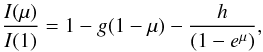 (5)and a more general law with four terms (Claret 2000)
 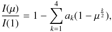 (6)where I(1) is the specific intensity at the centre of the disk, and u,a,b,c,d,e,f,g,h, and ak are the corresponding LDCs. The parameter μ is given by μ = cos(γ), where γ is the angle between the line of sight and the emergent intensity. The model atmosphere intensities were convolved with a response function that considers the filter transmission curves for Kepler, CoRoT, Spitzer(IRAC), uvby (Strömgren), UBVRIJHK (Johnson-Cousins), Sloan, and 2MASS, double reflection from an aluminium-coated mirror and detector sensitivity (see for example Eq. (7) in Claret & Hauschildt 2003). All calculations were performed by adopting the least-square method (LSM). In addition, to help users of a tool for evaluating the theoretical errors in the LDC, we also computed the coefficients by using the flux conservation method (FCM) for bi-parametric and linear approximations. Such a method conserves – by definition – the flux, but the corresponding fits give larger numerical scattering than the LSM.
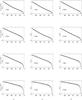 |
Fig. 1 The specific intensity distribution for a [4800, 4.5] spherical symmetric model. Continuous line represents the actual intensities while crosses denote the fit by adopting Eq. (6). Calculations for Strömgren and Johnson-Cousins photometric systems. |
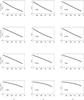 |
Fig. 2 The same as in Fig. 1 but for the case quasi-spherical. Crosses indicate the fit using Eq. (6). Calculations for Strömgren and Johnson-Cousins photometric systems. |
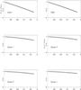 |
Fig. 3 The same as in Fig. 1 but for the case quasi-spherical. Crosses indicate the fit using Eq. (2). Calculations for Kepler, CoRot, and Spitzer (IRAC) photometric systems. |
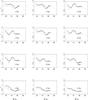 |
Fig. 4 Linear LDC for quasi-spherical calculations using drift-phoenix models (continuous lines, crosses), cond-phoenix (dashed lines), and atlas plane-parallel models (points). Log g = 4.0, solar composition, microturburlent velocity =2.0 km s-1, uvbyUBVRIJHK passbands. |
The non-linearity of the specific intensity distribution has been known for a long time (Kinglesmith & Sobieski 1970; Manduca et al. 1977; Díaz-Cordobés & Giménez 1992; Van Hamme 1993). Such a non-linear characteristic is even more pronounced in the case of spherical models due to the drop-offs that are caused by the decreased matter-radiation interaction near the extreme limb of the star. At first glance, the transfer equation for a spherically symmetric medium is significantly more complex than the corresponding plane-parallel geometry since it is a partial differential equation in r and μ. However, the use of the characteristic paths reduces the spacial operator to a single derivative with respect to the pathlength, and the spherical symmetric equation is not structurally different from the plane-parallel one (Mihalas 1978). Therefore, it is not surprising that both geometries provide similar results for some ranges of μ’s.
A spherical 1D model can be considered as having a core and an envelope. The core behaves very roughly like a plane-parallel structure and the envelope delivers the fully spherical part. Therefore, using only the core part is very similar to using a plane-parallel model. If we consider only the μ points previous to the drop-offs, the resulting shape of the intensity distribution is similar to those with the same Teff, log g, log [M/H] and mixing-length parameter but computed with plane-parallel geometry (see for example, Figs. 5 and 6 by Claret & Hauschildt 2003). Thus, a quasi-spherical model is defined as the one computed with spherical symmetry but without considering the drop-off region. The quasi-spherical models can be used, for example, in those situations for which the small intensities near the limb predicted by spherical models cannot be observationally detected or when the effects of sphericity are not important. The set of μ values in phoenix code depends on the characteristics of each model. After an inspection of the intensities profiles for each passband used here, we select as cut-off μ ≥ 0.1.
Another important point that must be considered and also justifies the use of quasi-spherical models is related to the observational difficulty of detecting the low intensities predicted by spherical models near the limb. Often, observations of extrasolar planet transits or double-lined eclipsing binaries, for example, are not yet able to detect these low intensities. In very favourable cases, only bi-parametric semi-empirical LDC are derived, at best. Nevertheless, the profiles of the intensities of the spherical models are complicated and cannot be described well by bi-parametric laws, thus hampering such a comparison. The use of the quasi-spherical models may also be useful in these situations given that bi-parametric laws such as Eqs. (2)−(5) can be applied with good results to these models. Of course, the spherical models are more physically relevant than quasi-spherical ones. As mentioned before, this concept is very useful when the low intensities near the limb cannot be detected and compared with the theoretical predictions.
Figure 1 shows the results for the uvbyUBVRIJHK photometric systems where the integrated intensity distribution is compared with the fits provided by Eq. (6) for a model with Teff = 4800 K and log g = 4.5. We denote a given model as [Teff, log g]. The drop-offs are much more pronounced for longer effective wavelengths, say, for the passbands RIJHK. Despite the complicated shape of the curves, it is clear that Eq. (6) represents the integrated intensity distributions very well. However, the agreement is not very good for longer effective wavelengths due to the corresponding steep behaviour of the drop-offs, although they are still acceptable.
When we consider quasi-spherical models, the agreement between the integrated intensities and the fits provided by Eq. (6) is still better than for pure spherical models due to the smoothness of profiles (Fig. 2). The bi-parametric approximations and even the linear one give fits similar to those obtained with plane-parallel models, as for example, those illustrated in Fig. 3 for the six passbands of Kepler, CoRot, and Spitzer (quadratic law). Comparisons between the quasi-spherical models generated by the phoenix code and those generated by the plane-parallel atlas (Kurucz, priv. comm.) confirm the utility of the mentioned concept (see below). On the other hand, the exponential equation fits the actual integrated intensities for all photometric systems well for spherical models. Therefore, Eq. (5) is useful for those users who wish to incorporate the effects of sphericity but using a law with only two terms, instead of with four terms as in Eq. (6). However, such a law should be used with caution as representative of pure spherical models because the corresponding fits are much more worse than those obtained with Eq. (6).
If we compare the present LDC with those previously computed using phoenix spherical models (Claret & Hauschildt 2003), we find good interagreement, except for the passbands u and U. However, this comparison was only possible for models with Teff ≈ 5000 K, given the ranges of effective temperatures of the two studies.
The linear fit, as mentioned, is not a good approximation for the intensity distributions. However, its simplicity makes it appropriate to comparing the present results for quasi-spherical models (cond-phoenix and drift-phoenix) with those generated with the atlas code. This is shown in Fig. 4 for the Strömgren and Johnson-Cousins systems. In general, the differences are smaller for higher Teff, except for the passbands v and U. More remarkable is the abrupt variation in the linear coefficients for effective temperatures around 2000 K for cond-phoenix models. This decrease is more pronounced for 5500 Å < λ < 8000 Å, i.e., for the filters y,V,R, and I. For wavelengths outside the mentioned interval, such variations are attenuated and practically disappear. These variations also depend on the local gravity, being less steep for lower log g. For the models drift-phoenix such variations disappear but we detected discontinuities around Teff ≈ 3000 K, which is inversely proportional to the wavelength. The aforementioned discontinuities probably are connected with the switch between cond-drift models. In general, the LDC computed using drift-phoenix models are greater than those derived by adopting cond-phoenix ones.
An interesting and important question concerning the comparison between theoretical and observational LDC is whether the cond and drift models are distinguishable with our actual level of observational accuracy. Figure 4 can be useful to help us shed some light on this point. The mean average error bars for semi-empirical linear LDC is approximately of 0.1, while for the quadratic approach they are around 0.2 for a and b (see for example, Southworth 2008; Claret 2009). In the linear case, the discrimination between cond and drift models seems to be possible, depending on the effective temperature and the adopted passband. It would be desirable that observers could perform such tests with the objective of providing some clues to the stellar atmosphere modellers in order to improve the theoretical models. Mutatis mutandis, the same applies to the bi-parametric approach.
As we have seen, no law describes the distribution of intensities perfectly. We have calculated the merit function for each fit that will help users decide which law to use. This function is given for all passbands (multiplied by the number of points μ used in each fit which is around 78). For interested users, we can also provide the actual intensity distribution (in normal μ points).
Limb-darkening coefficients for the Kepler, CoRoT, Spitzer, UBVRIJHK, uvby, Sloan, and 2MASS photometric systems.
4. Summary and final comments
We present the LDC for the spherical symmetric phoenix models atmosphere spanning a log g range between 2.5 and 5.5, solar metallicity, and effective temperatures 1500 K ≤ Teff ≤ 4800 K. Our coefficients cover the transmission curves of the Kepler, CoRoT, and Spitzer space missions and the usual Johnson-Cousins, Strömgren, Sloan, and 2MASS passbands.
We have adopted six equations to describe the specific intensities (linear, quadratic, root-square, logarithmic, exponential, and the one containing four terms). In case of pure spherical models, only the exponential equation and that containing four terms were used, while the bi-parametric and linear laws were used to describe the quasi-spherical. In the last cases, we also computed the LDC by adopting FCM to help estimate the theoretical error bars.
Table 1 summarises the results for the LDC calculations (Tables 2−25). These tables can be retrieved electronically at CDS. Finally, we are also able to provide LDC for additional photometric systems on request (for Walraven and Geneva photometric systems, we refer to Claret 2003).
Acknowledgments
We thank an anonymous referee for his/her comments and suggestions. The Spanish MEC (AYA2006-06375, AYA2009-14000-C03-01) is gratefully acknowledged for its support during the development of this work. This research made use of the SIMBAD database,operated at the CDS, Strasbourg, France, and of NASA’s Astrophysics Data System Abstract Service.
References
- Claret, A. 2000, A&A, 363, 1081 [NASA ADS] [Google Scholar]
- Claret, A. 2003, A&A, 401, 657 [NASA ADS] [CrossRef] [EDP Sciences] [Google Scholar]
- Claret, A. 2008, A&A, 482, 259 [NASA ADS] [CrossRef] [EDP Sciences] [Google Scholar]
- Claret, A. 2009, A&A, 506, 1335 [NASA ADS] [CrossRef] [EDP Sciences] [Google Scholar]
- Claret, A., & Hauschildt, P. H. 2003, A&A, 412, 241 [NASA ADS] [CrossRef] [EDP Sciences] [Google Scholar]
- Díaz-Cordovés, J., & Giménez, A. 1992, A&A, 259, 227 [NASA ADS] [Google Scholar]
- Fields, D. L., Albrow, M. D., An, J., et al. 2003, ApJ, 596, 1305 [NASA ADS] [CrossRef] [Google Scholar]
- Haubois, X., Perrin, G., Lacour, S., et al. 2009, A&A, 508, 923 [NASA ADS] [CrossRef] [EDP Sciences] [Google Scholar]
- Helling, Ch., Woitke, P., & Thi, W.-F. 2008, A&A, 485, 547 [NASA ADS] [CrossRef] [EDP Sciences] [Google Scholar]
- Howarth, I. D. 2011, MNRAS, 418, 1165 [NASA ADS] [CrossRef] [Google Scholar]
- Klinglesmith, D. A., & Sobieski, S. 1970, AJ, 75, 175 [NASA ADS] [CrossRef] [Google Scholar]
- Manduca, A., Bell, R. A., & Gustafsson, B. 1977, A&A, 61, 809 [NASA ADS] [Google Scholar]
- Mihalas, D. 1978, Stellar Atmospheres (San Francisco: W. H. Freeman and Company) [Google Scholar]
- Neilson, H. R., & Lester, J. B. 2008, A&A, 490, 807 [NASA ADS] [CrossRef] [EDP Sciences] [Google Scholar]
- Neilson, H. R., & Lester, J. B. 2011, A&A, 530, A65 [NASA ADS] [CrossRef] [EDP Sciences] [Google Scholar]
- Orosz, J. A., & Hauschildt, P. H. 2000, A&A, 364, 265 [NASA ADS] [Google Scholar]
- Rattenbury, N. J., Abe, F., Bennett, D. P., et al. 2005, A&A, 439, 645 [NASA ADS] [CrossRef] [EDP Sciences] [Google Scholar]
- Sing, D. K. 2010, A&A, 510, A21 [Google Scholar]
- Southworth, J. 2008, MNRAS, 386, 1644 [NASA ADS] [CrossRef] [Google Scholar]
- Van Hamme, W. 1993, AJ, 106, 2096 [NASA ADS] [CrossRef] [Google Scholar]
- Witte, S., Helling, Ch., & Hauschildt, P. H. 2009, A&A, 506, 1367 [NASA ADS] [CrossRef] [EDP Sciences] [Google Scholar]
- Witte, S., Helling, Ch., Barman, T., Heidrich, N., & Hauschildt, P. H. 2011, A&A, 529, A44 [NASA ADS] [CrossRef] [EDP Sciences] [Google Scholar]
- Wittkowski, M., Aufdenberg, J. P., & Kervella, P. 2004, A&A, 413, 711 [NASA ADS] [CrossRef] [EDP Sciences] [Google Scholar]
- Wittkowski, M., Hummel, C. A., Aufdenberg, J. P., & Roccatagliata, V. 2006a, A&A, 460, 843 [NASA ADS] [CrossRef] [EDP Sciences] [Google Scholar]
- Wittkowski, M., Aufdenberg, J. P., Driebe, T., et al. 2006b, A&A, 460, 855 [NASA ADS] [CrossRef] [EDP Sciences] [Google Scholar]
- Woitke, P., & Helling, C. 2004, A&A, 414, 335 [NASA ADS] [CrossRef] [EDP Sciences] [Google Scholar]
- Zub, M., Cassan, A., Heyrovsky, D., et al. 2011, A&A, 525, A15 [NASA ADS] [CrossRef] [EDP Sciences] [Google Scholar]
All Tables
Limb-darkening coefficients for the Kepler, CoRoT, Spitzer, UBVRIJHK, uvby, Sloan, and 2MASS photometric systems.
All Figures
|
Fig. 1 The specific intensity distribution for a [4800, 4.5] spherical symmetric model. Continuous line represents the actual intensities while crosses denote the fit by adopting Eq. (6). Calculations for Strömgren and Johnson-Cousins photometric systems. |
| In the text | |
|
Fig. 2 The same as in Fig. 1 but for the case quasi-spherical. Crosses indicate the fit using Eq. (6). Calculations for Strömgren and Johnson-Cousins photometric systems. |
| In the text | |
|
Fig. 3 The same as in Fig. 1 but for the case quasi-spherical. Crosses indicate the fit using Eq. (2). Calculations for Kepler, CoRot, and Spitzer (IRAC) photometric systems. |
| In the text | |
|
Fig. 4 Linear LDC for quasi-spherical calculations using drift-phoenix models (continuous lines, crosses), cond-phoenix (dashed lines), and atlas plane-parallel models (points). Log g = 4.0, solar composition, microturburlent velocity =2.0 km s-1, uvbyUBVRIJHK passbands. |
| In the text | |
Current usage metrics show cumulative count of Article Views (full-text article views including HTML views, PDF and ePub downloads, according to the available data) and Abstracts Views on Vision4Press platform.
Data correspond to usage on the plateform after 2015. The current usage metrics is available 48-96 hours after online publication and is updated daily on week days.
Initial download of the metrics may take a while.