| Issue |
A&A
Volume 546, October 2012
|
|
|---|---|---|
| Article Number | A93 | |
| Number of page(s) | 7 | |
| Section | The Sun | |
| DOI | https://doi.org/10.1051/0004-6361/201219795 | |
| Published online | 11 October 2012 | |
Spectroscopic observations of propagating disturbances in a polar coronal hole: evidence of slow magneto-acoustic waves
1
Max-Planck-Institut für Sonnensystemforschung (MPS),
37191
Katlenburg-Lindau,
Germany
e-mail: gupta@mps.mpg.de
2
Institute for Experimental and Applied Physics (IEAP), Christian
Albrechts University at Kiel, Kiel
24118,
Germany
3
School of Space Research, Kyung Hee University,
Yongin,
446-701
Gyeonggi,
Korea
4
Indian Institute of Astrophysics, 560034
Bangalore,
India
Received: 11 June 2012
Accepted: 11 September 2012
Aims. We focus on detecting and studying quasi-periodic propagating features that have been interpreted in terms of both slow magneto-acoustic waves and of high-speed upflows.
Methods. We analyzed long-duration spectroscopic observations of the on-disk part of the south polar coronal hole taken on 1997 February 25 by the SUMER spectrometer onboard SOHO. We calibrated the velocity with respect to the off-limb region and obtained time-distance maps in intensity, Doppler velocity, and line width. We also performed a cross-correlation analysis on different time series curves at different latitudes. We studied average spectral line profiles at the roots of propagating disturbances and along the propagating ridges, and performed a red-blue asymmetry analysis.
Results. We clearly find propagating disturbances in intensity and Doppler velocity with a projected propagation speed of about 60 ± 4.8 km s-1 and a periodicity of ≈14.5 min. To our knowledge, this is the first simultaneous detection of propagating disturbances in intensity as well as in Doppler velocity in a coronal hole. During the propagation, an intensity enhancement is associated with a blueshifted Doppler velocity. These disturbances are clearly seen in intensity also at higher latitudes (i.e., closer to the limb), while disturbances in Doppler velocity become faint there. The spectral line profiles averaged along the propagating ridges are found to be symmetric, to be well fitted by a single Gaussian, and have no noticeable red-blue asymmetry.
Conclusions. Based on our analysis, we interpret these disturbances in terms of propagating slow magneto-acoustic waves.
Key words: Sun: corona / Sun: transition region / Sun: UV radiation / Sun: oscillations / waves
© ESO, 2012
1. Introduction
Magnetohydrodynamic (MHD) waves are important candidates for the heating of the solar corona and the acceleration of the fast solar wind (Cranmer 2009; Ofman 2010). Recently, McIntosh et al. (2011a) reported the ubiquitous presence of outward-propagating transverse oscillations with amplitudes of nearly 20 km s-1 and periods between 100 s and 500 s throughout the quiescent atmosphere, which according to these authors are sufficiently energetic to accelerate the fast solar wind and heat the quiet corona. Numerous reports on the detection of various MHD wave modes in different parts of the solar atmosphere are present in the literature (Nakariakov & Verwichte 2005; Banerjee et al. 2007, 2011). Depending on the modes of propagation, these waves can give a variety of signatures in various spectral line profile parameters (Kitagawa et al. 2010). The propagation of slow magneto-acoustic waves in the upper solar atmosphere gives oscillations in intensity as well as in the Doppler velocity with a propagation speed slower than or equal to the sound speed (Byerley et al. 1978; Edwin & Roberts 1983). Based on these observational signatures, intensity oscillations with periods between 3 min and 30 min observed in polar coronal holes (e.g., DeForest & Gurman 1998; Ofman et al. 1999; Banerjee et al. 2009; Krishna Prasad et al. 2011) and in active region loops (e.g., Berghmans & Clette 1999; De Moortel et al. 2000, 2002; King et al. 2003; McEwan & de Moortel 2006; McIntosh et al. 2008; Marsh et al. 2009; Stenborg et al. 2011) were interpreted in terms of slow magneto-acoustic waves. From spectroscopic studies, similar oscillations were detected in intensity and Doppler velocity (e.g., O’Shea et al. 2001; Wang et al. 2003a,b; Gupta et al. 2009; Wang et al. 2009a,b; Mariska & Muglach 2010; Nishizuka & Hara 2011) and were, again, mostly interpreted as slow magneto-acoustic waves.
With imaging observations, propagating intensity disturbances with speeds between 50 km s-1 and 200 km s-1 detected in active regions (e.g., Sakao et al. 2007; Hara et al. 2008; McIntosh & De Pontieu 2009b) and in coronal holes (e.g., McIntosh et al. 2010; Tian et al. 2011b) were recently alternatively interpreted as recurrent high-speed upflows. At the same time, spectroscopic observations show asymmetries in the blue wing of transition region and coronal emission lines (e.g., De Pontieu et al. 2009; McIntosh & De Pontieu 2009a; De Pontieu & McIntosh 2010; McIntosh et al. 2011b; Tian et al. 2011a), which were attributed to the ubiquitous high-speed upflows in the observed regions. These upflows might be recurrent phenomena and would cause quasi-periodic oscillations in intensity, Doppler velocity, and width (De Pontieu & McIntosh 2010). Accordingly, interpreting the observed oscillations in terms of recurrent high-speed upflows has challenged the wave interpretation.
Coronal holes are the source region of the high-speed solar wind and are associated with rapidly expanding open magnetic fields (see review by Cranmer 2009). Cranmer & van Ballegooijen (2005) and Cranmer et al. (2007) described the role of MHD waves for the heating of the corona and for the acceleration of the solar wind in coronal holes. Moreover, high-speed outflows at the base of coronal holes can provide heated mass to the corona and the fast solar wind (McIntosh et al. 2010; Tian et al. 2011b). Thus, a detection of propagating disturbances in coronal holes would contribute to understanding the heating of the gas in the coronal hole and the acceleration of the fast solar wind, either in terms of propagating waves or high-speed flows or even as a superposition of both. In order to distinguish between these scenarios, good spectroscopic observations of these features are needed.
We focus on very long duration “sit-and-stare” mode spectroscopic observations of a polar coronal hole to identify propagating disturbances within our field of view and to study their nature. We also look for the source and physical events responsible for these disturbances and the observed periodicity. In addition, we tested the applicability of the red-blue (R − B) asymmetry analysis to our dataset.
2. Data reduction and analysis
The data analyzed here were obtained on 1997 February 25 in the south polar coronal hole in “sit-and-stare” mode with the Solar Ultraviolet Measurement of Emitted Radiation (SUMER, Wilhelm et al. 1995) onboard SOHO. Two-thirds of the SUMER slit were placed on-disk, whereas the remaining part was off-limb. Observations started at 00:00 UT and ended at around 14:00 UT with an exposure time of 60 s, recording the Ne viii 770 Å and N iv 765 Å spectral lines in the first order of diffraction on detector B. Figure 1 shows the location of the SUMER slit in an image of the south polar coronal hole taken in the 195 Å passband with the Extreme ultraviolet Imaging Telescope (EIT, Delaboudinière et al. 1995) onboard SOHO. Scullion et al. (2009) also analyzed the same dataset to identify and characterize jet events.
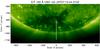 |
Fig. 1 EIT/SOHO 195 Å context image of the southern polar coronal hole showing the location of the SUMER slit. |
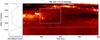 |
Fig. 2 Left panel: the normalized time-averaged intensity variation along the slit. Right panel: the intensity variation along solar-Y with time, which is normalized by the time-averaged intensity variation along the slit. The white dashed line marks the location of maximum limb brightening, whereas the continuous box indicates the region chosen for detailed analysis. |
Data were first decompressed, corrected for dead-time, response inhomogeneities (flat-field), local-gain depression, and for geometrical distortion (de-stretching), using the routines provided in SolarSoft. Single Gaussian fits were applied to obtain the line peak, Doppler shift, and width of each spectrum, thus obtaining distance-time (Y − T) maps of all three line parameters. These maps show horizontal stripes due to residuals in the flat-field correction. Additionally, the Doppler shift Y − T map shows slow variations with time due to changes in the instrument temperature during the 14 h duration of the observations and a trend along the slit due to residuals from the distortion correction. Intensity and line width maps were divided by the normalized time-averaged profile along the slit. In the case of the Ne viii 770 Å Doppler shift map, the correction requires more care to retain the variations along the slit that are of solar origin (e.g., center-to-limb variations). The medium and large-scale variations along the slit due to residuals in the distortion correction was obtained from far-off-limb spectra in cold lines (pure stray-light), which were taken two days before at nearly the same detector position and were then subtracted from the data. Small-scale (few pixels) residual effects were removed by additionally dividing the velocity map by the normalized, high-pass-filtered, time-averaged profile along the slit. Finally, to convert the Doppler shifts into absolute Doppler velocities, we set the average Doppler velocity in the off-limb part (between solar-Y ≈ −990″ and −1050″) to zero in each frame (line-of-sight (LOS) motions are expected to average out above the limb in an optically thin plasma, Doschek et al. 1976). This procedure also removes the temporal variation along the wavelength scale due to the changes in the instrument temperature. The Doppler velocity calibrated in this way gives an average outflow speed of about 2.5 km s-1 in Ne viii in the on-disk polar coronal hole, consistent with previous studies at similar latitudes (e.g., Wilhelm et al. 2000). Figure 2 shows the resulting Y − T map obtained in normalized Ne viii 770 Å intensity. The left panel displays the normalized intensity variation along the slit. Many propagating disturbances (slanted ridges) in the on-disk part of the Y − T map can be seen in the right panel of Fig. 2. We identified one such region where these propagating disturbances are very clearly seen in most of the line parameters. This region is outlined with a white box on the intensity Y − T map of Fig. 2. For the remaining part of this paper we will focus our attention on this region. To see these propagating disturbances more clearly, one needs to remove any low-frequency changes in intensity, Doppler velocity, and width from the time series. To do this, we smoothed all three Y − T maps using the boxcar size of [3, 20] in pixel units and then subtracted it from the original maps. To derive the relative change in intensity and width, we divided these quantities by the smoothed map, obtaining the resulting enhanced Y − T maps as shown in Fig. 3. Thus, the applied processing can be summarized as δL(t,y) = (L(t,y) – *error*¯L(t,y))/ L¯(t,y) and δv(t,y) = v(t,y) – v¯(t,y), where L stands for either intensity or line width, v for velocity, and L¯ and v¯ are the smoothed parameters.
The solar rotation at X ≈ 0″, at date of observation, extends from 2.8″/h at Y ≈ −840″ to 1″/h at Y ≈ −940″. These values are comparable with, or smaller than, the SUMER spatial resolution of 2″ (Lemaire et al. 1997), ensuring that the same location is observed for an adequate period of time.
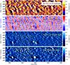 |
Fig. 3 Enhanced distance-time map of the intensity (top panel), Doppler velocity (upper middle panel), and line width (lower middle panel) of the Ne viii 770 Å spectral line, and map of the line width (lower panel) of the N iv 765 Å spectral line. Propagating disturbances moving toward the limb are clearly visible in the top and middle panels and have a propagation speed of 60 ± 4.8 km s-1. White and black continuous lines in the top two panels are drawn to trace propagating disturbances with a period of 14.5 min. The bottom panel shows significant enhancements in line width at lower heights in the solar atmosphere at the base of the propagating disturbances (marked with ellipses). |
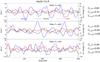 |
Fig. 4 Time series of Ne viii 770 Å spectral line intensity, Doppler velocity, and width, which are obtained from Y − T maps at three different locations averaged over three spatial pixels. The measured Doppler shifts are shown in km s-1, while the other parameters are given in relative percentage change. The zero-velocity line is also plotted to distinguish between red and blueshifts. Linear correlation coefficients between different nondetrended time series curves are provided for each latitude on the right side of each frame. The 95% and 99% confidence level for linear correlation coefficients are about 0.217 and 0.284, respectively. |
3. Results and discussion
Distance-time maps of intensity and velocity (Fig. 3) clearly reveal propagating disturbances with 5% to 10% variations in intensity and 3 km s-1 to 6 km s-1 changes in the Doppler velocity. To our knowledge, this is the first simultaneous detection of propagating disturbances in intensity and Doppler velocity in a coronal hole region, in contrast to earlier detections, which were restricted to active regions (Wang et al. 2009b; Tian et al. 2011a; Nishizuka & Hara 2011). The slanted bright and dark ridges (blue and red, in case of Doppler velocity) in the top two panels of Fig. 3 are found to move toward the limb (i.e., outward from the Sun) with a projected propagation speed of 60 ± 4.8 km s-1. In both panels, white and black continuous lines indicate the expected trajectories of disturbances propagating at ≈60 km s-1 and with a 14.5 min periodicity. Clearly, enhancements in intensity are associated with blueshifts (i.e., motion away from the Sun), whereas reductions in intensity are associated with redshifts (inward motion). The speeds measured here are comparable to previously reported ones from Ne viii 770 Å in a polar coronal hole, but off-limb (Banerjee et al. 2009). Comparing all Y − T maps, we deduce that these propagating disturbances are best visible in the zeroth moment of the spectral line (line intensity) followed closely by their visibility in Doppler velocity, but are less clearly evident in line width. In the velocity Y − T map, these propagating disturbances are seen better at lower latitudes and become fainter at higher latitudes (closer to the limb). This result explains why previous studies at higher latitudes and off-limb in polar coronal holes with the same Ne viii 770 Å spectral line did not detect these disturbances in Doppler velocities, but only in intensity (Banerjee et al. 2009; Gupta et al. 2010).
To demonstrate the typical phase relationships between different spectral line parameters, the time series, as obtained for all three parameters, are plotted in Fig. 4 at three different latitudes. The anticorrelation between intensity and Doppler velocity and the correlation between intensity and Doppler width are best seen in the top panel, but partly persist also at higher latitudes (lower panels). The strongest anticorrelation is between intensity and velocity (above 99% confidence level at almost all latitudes), followed by the positive correlation between intensity and line width (above 95% confidence level at almost all latitudes). However, here we wish to point out that error bars associated with line width from Gaussian fitting are larger than the amplitude of their variations, hence, no major conclusion can be drawn from the line width part. Moreover, there is no correlation observed between Doppler width and red-blue asymmetry maps obtained from the Ne viii 770 Å spectral profiles.
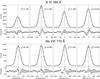 |
Fig. 5 Averaged spectral line profiles of N iv 765 Å at the root of the propagating disturbances (top panels) at the four epochs of enhanced width in N iv (see bottom panel of Fig. 3) and (bottom panels) over the top quarter of the corresponding blueshifted ridges in Ne viii (see second panel of Fig. 3). Profiles are plotted in the order of their occurrence in time. Both the N iv 765 Å and Ne viii 770 Å observed spectral profiles (solid histograms) are fitted with a single Gaussian component and constant background (dashed lines). The bars in the residual panels indicate the uncertainties of the measurement. Velocity scales are calibrated with respect to averaged off-limb wavelength. Vertical dashed lines in all panels mark the position of the fitted line centroid. |
Recently, Wang et al. (2009a) and Verwichte et al. (2010) showed that the phase at which an outward propagating slow magneto-acoustic wave produces a blueshift of the line profile coincides with a density (i.e., intensity) enhancement, in agreement with Figs. 3 and 4. According to the distance-time (Y − T) maps in Fig. 3 and the time series curves in Fig. 4, the enhancement in intensity is associated with a Doppler blueshift. Therefore, these disturbances are consistent with an upward propagating slow magneto-acoustic wave (Wang et al. 2009a). Moreover, a projected propagation speed of about 60 ± 4.8 km s-1 is subsonic (the sound speed CS ≈ 120 km s-1 at the Ne viii 770 Å formation temperature of 630 000 K).
If these propagating disturbances were caused by periodic plasma upflows, we would expect that the highly blueshifted velocity (about 10 km s-1 to 18 km s-1 along the LOS for a radial structure making an angle of about 10° with the plane of sky at these latitudes for upflows between 60 km s-1 to 100 km s-1) associated to this upflow be on the top of average, slightly blueshifted continuous outflow typically seen in Ne viii in coronal holes. At the lower latitudes at which the disturbances are seen, the continuous outflow speeds are slow and true redshifts are observed at some phases of the wave. This finding supports the notion that these propagating disturbances correspond to waves. However, we caution that this result sensitively depends on velocity calibration, and the difficulty of EUV wavelength calibration reduces its reliability.
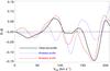 |
Fig. 6 Variation of the R − B asymmetry of line profiles with velocities measured from the respective line centroid (VRB). The continuous black curve is obtained from the observed profile of Ne viii 770 Å shown in the first bottom panel of Fig. 5. The red and blue curves are obtained from the simulated profile modeled with a single Gaussian and a constant background (with parameters similar to the observed profile) but sampled differently with respect to the line centroid. The red curve represents the case of maximum asymmetry in sampling (about half a pixel shift from the line centroid) while the blue curve is sampled symmetrically and therefore shows just the effects of noise. |
We also looked for signatures of these disturbances in the transition region (N iv 765 Å) to find indications of the physical event and source responsible for these disturbances. We could not find any propagating signature in any of the line parameters of N iv 765 Å. However, the line width of N iv 765 Å is enhanced at the location from where these propagating disturbances in Ne viii 770 Å originate (bottom panel of Fig. 3). More precisely, patches of enhanced width of the N iv 765 Å line appear to correspond to the blueshifted phase of the Ne viii 770 Å line (see Fig. 3). This enhanced width at lower height indicates either unresolved small-scale reconnections associated with explosive events (Innes et al. 1997) happening at that place as evident from associated line width enhancement and Doppler blueshift of N iv 765 Å profiles, or a local increase in turbulence. Thus, it may be possible that these propagating disturbances are triggered by these small-scale events that cause the increased line width of transition region lines. However, the reverse can also be true, with a periodic burst of explosive events triggered by the waves, as has been proposed by Ning et al. (2004). Note that a relatively small increase in line width suggests that either these are rather weak explosive events, or that the enhancement in line width has a different cause.
To check the influence of the propagating disturbances on the spectral line profiles, we plot in the upper row of Fig. 5 the averaged line profiles of N iv 765 Å at the root of the propagating disturbances, i.e., at the locations at which N iv 765 Å displays an enhanced line width (the plotted profiles are summed over the areas marked with white ellipses in the bottom panel of Fig. 3). In the lower row of Fig. 5, we plot Ne viii 770 Å profiles summed along the top quarter (low latitudes) of the propagating ridge, where enhancements in intensity and blueshifted velocities are clearly visible in Ne viii 770 Å. The resulting profiles are ordered according to increasing time from left to right in Fig. 5. Each plotted profile is fitted with a single Gaussian and a constant background. The fit residuals are also plotted. The average reduced chi-square,  , of four fits at the root of the propagating disturbances (in N iv 765 Å) is about 1.65 and, together with the relatively consistent shape of the residual in all four profiles indicates the presence of a small blueshifted component (confirmed by a double Gaussian fit), which is particularly clearly evident in the fourth panel from the left. The average of about 0.88 and shapes of the residuals together show, however, that the Ne viii profiles averaged over the blueshifted ridges are well represented by a single Gaussian and leave little room for a significant second component. The presence of only one component may indicate that in this observation the background emission is weak, and most of the emission is coming from the oscillating coronal structure.
In general, it is very difficult to uniquely fit two Gaussian components to all spectral profiles for the whole sequence. These fits have multiple solutions, with the final solution depending on the initial guess of the line parameters and also on the constraints applied to the fit. Accordingly, multi-Gaussian fittings with a unique set of initial guess parameters and constraints do not lead to conclusive result.
To further check for the presence of a second component, we also applied the R − B asymmetry analysis to all Ne viii 770 Å spectral line profiles. After obtaining the line centroids from a single Gaussian fit, the line profiles were interpolated using linear and spline methods to a spectral spacing ten times finer than the original one. We calculated the R − B asymmetry at different velocities (VRB) measured from the respective line centroid by using the formula (after De Pontieu & McIntosh 2010) 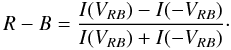 (1)Here we integrated the intensity (I) of the interpolated profile over a narrow spectral range (≈± 1.7 km s-1) at velocity (VRB). Values of the ratio in Eq. (1) give asymmetries whose sign fluctuates at different VRB and from profile to profile, indicating no clear preference for a stronger red and blue wing. The R − B asymmetry maps did not reveal propagating signatures in any of the velocity bins. Yet individual line profiles, such as along the ridges of the propagating disturbance, still show an R − B asymmetry with maximum amplitude of ± 0.07 for VRB ≤ 150 km s-1. Verwichte et al. (2010) pointed out the blueward and redward asymmetry in the line profiles at crest and trough epochs of wave propagation, respectively. However, in our dataset we did not find any such preferred asymmetry in the line profiles at any point or epoch.
To test whether the resulting R − B asymmetry values are significant and of solar origin, we performed a similar analysis on simulated line profiles. We generated a symmetric line profile (single Gaussian with constant background) with amplitude and FWHM similar to those in our dataset, but with spectral resolution ten times finer than the SUMER resolution. Finally, we added random noise to the signal in each data point, assuming a Poisson distribution. From this high-resolution profile, we extracted several profiles with spectral sampling similar to SUMER by sampling every tenth data point with different starting points. Finally, we performed an identical R − B analysis on these simulated line profiles as on the observations. The resulting R − B asymmetry profile shows red and blue wing asymmetries, respectively with amplitudes similar to those obtained from the observed profiles (see Fig. 6), although the modeled profile was completely symmetric, only sampled unsymmetrically. The effect apparently arises from the finite sampling of the data and is very susceptible to noise. Indeed, the amplitude of the asymmetry increases with velocity as the fractional error in the data points increases when moving away from the line centroid. The R − B asymmetry profile obtained from this analysis is similar to the R − B asymmetry profile obtained from the real data in terms of amplitude and sign of asymmetry (maximum amplitude is about ± 0.08 for VRB ≤ 150 km s-1 for the modeled profiles, see Fig. 6). Thus, we conclude that within the given signal-to-noise ratio and spectral sampling of our data, the R − B asymmetry analysis cannot detect any reliable secondary component. This finding supports the result that the Ne viii 770 Å line profiles associated with propagating disturbances are essentially symmetric in nature.
De Pontieu & McIntosh (2010) have shown that a single Gaussian fit to a spectral profile, having a quasi-periodically varying additional faint component of blueshift emission, can result in quasi-periodic modulation of the peak intensity, centroid, and width of a line, and thus could produce a small oscillatory signature in these line parameters. However, in our analysis we find the Doppler velocity amplitude of these disturbances to be relatively large at low latitudes, i.e., ± 3 km s-1 (on the top of average plasma outflow speed), which is much larger than that resulting from the simulations (about 1 km s-1) of De Pontieu & McIntosh (2010). Indeed, the above simulations could produce larger Doppler shifts by assuming a relatively strong second component that would, however, contradict the rather low intensity increases we observe. Tian et al. (2011a) investigated at the base of a loop and found in-phase intensity, Doppler velocity, and line-width variations and interpreted those to be due to fast flows. Nishizuka & Hara (2011) also researched at greater heights from the same loop footpoint and interpreted the propagating disturbances in terms of slow magneto-acoustic waves based on similar large-amplitude Doppler velocity oscillations (5 km s-1 peak-to-peak) with a noticeably correlated intensity and Doppler velocity and lack of evidence of blueward asymmetry in the line profiles. In our observations, the results are very similar to those obtained by Nishizuka & Hara (2011), and thus appear to support the conventional interpretation of these disturbances in terms of slow magneto-acoustic waves, as was done by Marsh et al. (2011) based on the measured subsonic speed of propagation. Moreover, a recent 3D MHD model of hot coronal loops developed by Ofman et al. (2012) shows the close relationship between slow waves and impulsive upflows at the loop footpoints that were generated by the same impulsive events. Clearly, to distinguish between slow waves and quasi-periodic upflows, a detailed analysis of the relationship between different oscillation parameters (e.g., period, phase speed, phase relations, damping time, and length) and loop parameters (e.g., loop length, density, temperature, and magnetic field) are required as demonstrated and pointed out by Ofman et al. (2012).
4. Conclusion
In summary, we found propagating disturbances in a polar coronal hole revealed by the intensity, velocity, and line width of the Ne viii 770 Å spectral line, with a projected propagation speed of 60 ± 4.8 km s-1 and a period ≈14.5 min. The observed disturbances show quasi-periodic enhancement in intensity in phase with the Doppler blueshift. At lower latitudes, true redshifts are also observed at some phases of the propagation. We studied Ne viii spectral line profiles averaged along the propagating ridges and found them to be symmetric, to be well-fitted by a single Gaussian, and to have no noticeable red-blue asymmetry. Based on our observations and analysis, we conclude that the most likely cause for these propagating disturbances in coronal hole regions are slow magneto-acoustic waves. Observations at lower heights in the solar atmosphere with the N iv 765 Å spectral line do not show any propagating features in any line parameter. However, it indicates that these waves may be caused by small-scale reconnections or explosive events occurring at the base of the propagating features. With the given propagation speed and velocity amplitude of these waves, the energy flux carried by them is far lower than needed for the heating of the solar corona (Wang et al. 2009a; Kitagawa et al. 2010). However, these waves may provide additional momentum for the acceleration of the fast solar wind in coronal holes (Ofman 2010) and their dissipation could also lead to extended heating of the outer coronal holes.
Acknowledgments
This work was partially supported by the Indo-German DST-DAAD joint project D/07/03045. The SUMER project is financially supported by DLR, CNES, NASA, and the ESA PRODEX programme (Swiss contribution). This work was partially supported by the WCU grant No. R31-10016 from the Korean Ministry of Education, Science and Technology.
References
- Banerjee, D., Erdélyi, R., Oliver, R., & O’Shea, E. 2007, Sol. Phys., 246, 3 [NASA ADS] [CrossRef] [Google Scholar]
- Banerjee, D., Teriaca, L., Gupta, G. R., et al. 2009, A&A, 499, L29 [NASA ADS] [CrossRef] [EDP Sciences] [Google Scholar]
- Banerjee, D., Gupta, G. R., & Teriaca, L. 2011, Space Sci. Rev., 158, 267 [NASA ADS] [CrossRef] [Google Scholar]
- Berghmans, D., & Clette, F. 1999, Sol. Phys., 186, 207 [NASA ADS] [CrossRef] [Google Scholar]
- Byerley, A., McWhirter, R. W. P., & Wilson, R. 1978, J. Phys. B At. Mol. Phys., 11, 613 [NASA ADS] [CrossRef] [Google Scholar]
- Cranmer, S. R. 2009, Liv. Rev. Sol. Phys., 6, 3 [Google Scholar]
- Cranmer, S. R., & van Ballegooijen, A. A. 2005, ApJS, 156, 265 [NASA ADS] [CrossRef] [Google Scholar]
- Cranmer, S. R., van Ballegooijen, A. A., & Edgar, R. J. 2007, ApJS, 171, 520 [Google Scholar]
- De Moortel, I., Ireland, J., & Walsh, R. W. 2000, A&A, 355, L23 [NASA ADS] [Google Scholar]
- De Moortel, I., Ireland, J., Walsh, R. W., & Hood, A. W. 2002, Sol. Phys., 209, 61 [NASA ADS] [CrossRef] [Google Scholar]
- De Pontieu, B., & McIntosh, S. W. 2010, ApJ, 722, 1013 [NASA ADS] [CrossRef] [Google Scholar]
- De Pontieu, B., McIntosh, S. W., Hansteen, V. H., & Schrijver, C. J. 2009, ApJ, 701, L1 [NASA ADS] [CrossRef] [Google Scholar]
- DeForest, C. E., & Gurman, J. B. 1998, ApJ, 501, L217 [NASA ADS] [CrossRef] [Google Scholar]
- Delaboudinière, J., Artzner, G. E., Brunaud, J., et al. 1995, Sol. Phys., 162, 291 [NASA ADS] [CrossRef] [Google Scholar]
- Doschek, G. A., Bohlin, J. D., & Feldman, U. 1976, ApJ, 205, L177 [NASA ADS] [CrossRef] [Google Scholar]
- Edwin, P. M., & Roberts, B. 1983, Sol. Phys., 88, 179 [NASA ADS] [CrossRef] [Google Scholar]
- Gupta, G. R., O’Shea, E., Banerjee, D., Popescu, M., & Doyle, J. G. 2009, A&A, 493, 251 [NASA ADS] [CrossRef] [EDP Sciences] [Google Scholar]
- Gupta, G. R., Banerjee, D., Teriaca, L., Imada, S., & Solanki, S. 2010, ApJ, 718, 11 [NASA ADS] [CrossRef] [Google Scholar]
- Hara, H., Watanabe, T., Harra, L. K., et al. 2008, ApJ, 678, L67 [NASA ADS] [CrossRef] [Google Scholar]
- Innes, D. E., Inhester, B., Axford, W. I., & Wilhelm, K. 1997, Nature, 386, 811 [NASA ADS] [CrossRef] [Google Scholar]
- King, D. B., Nakariakov, V. M., Deluca, E. E., Golub, L., & McClements, K. G. 2003, A&A, 404, L1 [NASA ADS] [CrossRef] [EDP Sciences] [Google Scholar]
- Kitagawa, N., Yokoyama, T., Imada, S., & Hara, H. 2010, ApJ, 721, 744 [NASA ADS] [CrossRef] [Google Scholar]
- Krishna Prasad, S., Banerjee, D., & Gupta, G. R. 2011, A&A, 528, L4 [NASA ADS] [CrossRef] [EDP Sciences] [Google Scholar]
- Lemaire, P., Wilhelm, K., Curdt, W., et al. 1997, Sol. Phys., 170, 105 [NASA ADS] [CrossRef] [Google Scholar]
- Mariska, J. T., & Muglach, K. 2010, ApJ, 713, 573 [NASA ADS] [CrossRef] [Google Scholar]
- Marsh, M. S., Walsh, R. W., & Plunkett, S. 2009, ApJ, 697, 1674 [NASA ADS] [CrossRef] [Google Scholar]
- Marsh, M. S., De Moortel, I., & Walsh, R. W. 2011, ApJ, 734, 81 [NASA ADS] [CrossRef] [Google Scholar]
- McEwan, M. P., & de Moortel, I. 2006, A&A, 448, 763 [NASA ADS] [CrossRef] [EDP Sciences] [Google Scholar]
- McIntosh, S. W., & De Pontieu, B. 2009a, ApJ, 707, 524 [NASA ADS] [CrossRef] [Google Scholar]
- McIntosh, S. W., & De Pontieu, B. 2009b, ApJ, 706, L80 [NASA ADS] [CrossRef] [Google Scholar]
- McIntosh, S. W., de Pontieu, B., & Tomczyk, S. 2008, Sol. Phys., 252, 321 [NASA ADS] [CrossRef] [Google Scholar]
- McIntosh, S. W., Innes, D. E., de Pontieu, B., & Leamon, R. J. 2010, A&A, 510, L2 [NASA ADS] [CrossRef] [EDP Sciences] [Google Scholar]
- McIntosh, S. W., de Pontieu, B., Carlsson, M., et al. 2011a, Nature, 475, 477 [NASA ADS] [CrossRef] [Google Scholar]
- McIntosh, S. W., Leamon, R. J., & De Pontieu, B. 2011b, ApJ, 727, 7 [NASA ADS] [CrossRef] [Google Scholar]
- Nakariakov, V. M., & Verwichte, E. 2005, Liv. Rev. Sol. Phys., 2, 3 [Google Scholar]
- Ning, Z., Innes, D. E., & Solanki, S. K. 2004, A&A, 419, 1141 [NASA ADS] [CrossRef] [EDP Sciences] [Google Scholar]
- Nishizuka, N., & Hara, H. 2011, ApJ, 737, L43 [NASA ADS] [CrossRef] [Google Scholar]
- Ofman, L. 2010, Liv. Rev. Sol. Phys., 7, 4 [Google Scholar]
- Ofman, L., Nakariakov, V. M., & DeForest, C. E. 1999, ApJ, 514, 441 [NASA ADS] [CrossRef] [Google Scholar]
- Ofman, L., Wang, T. J., & Davila, J. M. 2012, ApJ, 754, 111 [NASA ADS] [CrossRef] [Google Scholar]
- O’Shea, E., Banerjee, D., Doyle, J. G., Fleck, B., & Murtagh, F. 2001, A&A, 368, 1095 [NASA ADS] [CrossRef] [EDP Sciences] [Google Scholar]
- Sakao, T., Kano, R., Narukage, N., et al. 2007, Science, 318, 1585 [NASA ADS] [CrossRef] [PubMed] [Google Scholar]
- Scullion, E., Popescu, M. D., Banerjee, D., Doyle, J. G., & Erdélyi, R. 2009, ApJ, 704, 1385 [NASA ADS] [CrossRef] [Google Scholar]
- Stenborg, G., Marsch, E., Vourlidas, A., Howard, R., & Baldwin, K. 2011, A&A, 526, A58 [NASA ADS] [CrossRef] [EDP Sciences] [Google Scholar]
- Tian, H., McIntosh, S. W., & De Pontieu, B. 2011a, ApJ, 727, L37 [NASA ADS] [CrossRef] [Google Scholar]
- Tian, H., McIntosh, S. W., Rifal Habbal, S., & He, J. 2011b, ApJ, 736, 130 [NASA ADS] [CrossRef] [Google Scholar]
- Verwichte, E., Marsh, M., Foullon, C., et al. 2010, ApJ, 724, L194 [NASA ADS] [CrossRef] [Google Scholar]
- Wang, T. J., Solanki, S. K., Curdt, W., et al. 2003a, A&A, 406, 1105 [NASA ADS] [CrossRef] [EDP Sciences] [Google Scholar]
- Wang, T. J., Solanki, S. K., Innes, D. E., Curdt, W., & Marsch, E. 2003b, A&A, 402, L17 [NASA ADS] [CrossRef] [EDP Sciences] [Google Scholar]
- Wang, T. J., Ofman, L., & Davila, J. M. 2009a, ApJ, 696, 1448 [NASA ADS] [CrossRef] [Google Scholar]
- Wang, T. J., Ofman, L., Davila, J. M., & Mariska, J. T. 2009b, A&A, 503, L25 [NASA ADS] [CrossRef] [EDP Sciences] [Google Scholar]
- Wilhelm, K., Curdt, W., Marsch, E., et al. 1995, Sol. Phys., 162, 189 [NASA ADS] [CrossRef] [Google Scholar]
- Wilhelm, K., Dammasch, I. E., Marsch, E., & Hassler, D. M. 2000, A&A, 353, 749 [NASA ADS] [Google Scholar]
All Figures
|
Fig. 1 EIT/SOHO 195 Å context image of the southern polar coronal hole showing the location of the SUMER slit. |
| In the text | |
|
Fig. 2 Left panel: the normalized time-averaged intensity variation along the slit. Right panel: the intensity variation along solar-Y with time, which is normalized by the time-averaged intensity variation along the slit. The white dashed line marks the location of maximum limb brightening, whereas the continuous box indicates the region chosen for detailed analysis. |
| In the text | |
|
Fig. 3 Enhanced distance-time map of the intensity (top panel), Doppler velocity (upper middle panel), and line width (lower middle panel) of the Ne viii 770 Å spectral line, and map of the line width (lower panel) of the N iv 765 Å spectral line. Propagating disturbances moving toward the limb are clearly visible in the top and middle panels and have a propagation speed of 60 ± 4.8 km s-1. White and black continuous lines in the top two panels are drawn to trace propagating disturbances with a period of 14.5 min. The bottom panel shows significant enhancements in line width at lower heights in the solar atmosphere at the base of the propagating disturbances (marked with ellipses). |
| In the text | |
|
Fig. 4 Time series of Ne viii 770 Å spectral line intensity, Doppler velocity, and width, which are obtained from Y − T maps at three different locations averaged over three spatial pixels. The measured Doppler shifts are shown in km s-1, while the other parameters are given in relative percentage change. The zero-velocity line is also plotted to distinguish between red and blueshifts. Linear correlation coefficients between different nondetrended time series curves are provided for each latitude on the right side of each frame. The 95% and 99% confidence level for linear correlation coefficients are about 0.217 and 0.284, respectively. |
| In the text | |
|
Fig. 5 Averaged spectral line profiles of N iv 765 Å at the root of the propagating disturbances (top panels) at the four epochs of enhanced width in N iv (see bottom panel of Fig. 3) and (bottom panels) over the top quarter of the corresponding blueshifted ridges in Ne viii (see second panel of Fig. 3). Profiles are plotted in the order of their occurrence in time. Both the N iv 765 Å and Ne viii 770 Å observed spectral profiles (solid histograms) are fitted with a single Gaussian component and constant background (dashed lines). The bars in the residual panels indicate the uncertainties of the measurement. Velocity scales are calibrated with respect to averaged off-limb wavelength. Vertical dashed lines in all panels mark the position of the fitted line centroid. |
| In the text | |
|
Fig. 6 Variation of the R − B asymmetry of line profiles with velocities measured from the respective line centroid (VRB). The continuous black curve is obtained from the observed profile of Ne viii 770 Å shown in the first bottom panel of Fig. 5. The red and blue curves are obtained from the simulated profile modeled with a single Gaussian and a constant background (with parameters similar to the observed profile) but sampled differently with respect to the line centroid. The red curve represents the case of maximum asymmetry in sampling (about half a pixel shift from the line centroid) while the blue curve is sampled symmetrically and therefore shows just the effects of noise. |
| In the text | |
Current usage metrics show cumulative count of Article Views (full-text article views including HTML views, PDF and ePub downloads, according to the available data) and Abstracts Views on Vision4Press platform.
Data correspond to usage on the plateform after 2015. The current usage metrics is available 48-96 hours after online publication and is updated daily on week days.
Initial download of the metrics may take a while.