| Issue |
A&A
Volume 546, October 2012
|
|
|---|---|---|
| Article Number | A3 | |
| Number of page(s) | 12 | |
| Section | Interstellar and circumstellar matter | |
| DOI | https://doi.org/10.1051/0004-6361/201219659 | |
| Published online | 27 September 2012 | |
A hydrodynamic study of the circumstellar envelope of α Scorpii⋆
Hamburger Sternwarte, Universität Hamburg, Gojenbergsweg 112, 21029 Hamburg, Germany
e-mail: This email address is being protected from spambots. You need JavaScript enabled to view it.
; This email address is being protected from spambots. You need JavaScript enabled to view it.
Received: 23 May 2012
Accepted: 24 August 2012
Abstract
Context. Both the absolute mass-loss rates and the mechanisms that drive the mass loss of late-type supergiants are still not well known. Binaries such as α Sco provide the most detailed empirical information about the winds of these stars.
Aims. Our goal was to improve the binary technique for the determination of the mass-loss rate of α Sco A by including a realistic density distribution and velocity field from hydrodynamic and plasma simulations.
Methods. We performed 3D hydrodynamic simulations of the circumstellar envelope of α Sco in combination with plasma simulations accounting for the heating, ionization, and excitation of the wind by the radiation of α Sco B. These simulations served as the basis for an examination of circumstellar absorption lines in the spectrum of α Sco B as well as of emission lines from the Antares nebula.
Results. The present model of the extended envelope of α Sco reproduces some of the structures that were observed in the circumstellar absorption lines in the spectrum of α Sco B. Our theoretical density and velocity distributions of the outflow deviate considerably from a spherically expanding model, which was used in previous studies. This results in a higher mass-loss rate of (2 ± 0.5) × 10-6 M⊙ yr-1. The hot H ii region around the secondary star induces an additional acceleration of the wind at large distances from the primary, which is seen in absorption lines of Ti ii and Cr ii at −30 km s-1.
Key words: hydrodynamics / circumstellar matter / binaries: visual / stars: individual:αScorpii / stars: late-type / stars: mass-loss
Based on observations collected at the European Organisation for Astronomical Research in the Southern Hemisphere, Chile, under program ID 076.D-0690(A), and on observations made with the NASA/ESA Hubble Space Telescope (program # 5952), obtained at the Space Telescope Science Institute, which is operated by the Association of Universities for Research in Astronomy, Inc., under NASA contract NAS 5-26555.
© ESO, 2012
1. Introduction
In the late stage of the stellar evolution stars suffer a substantial mass loss by a continuous wind. This phenomenon plays a key role for the final development of individual stars and for the enrichment of the interstellar medium. However, the physical mechanisms that govern the outflow of late-type giants and supergiants are not established. Possible driving mechanisms include Alfvén waves, acoustic waves, shock waves, and pulsations (see the reviews of Lafon & Berruyer 1991; Willson 2000). As it is hard to distinguish between different driving mechanisms from a theoretical point of view, there is still a need for empirical studies to provide constraints.
The most accurate mass-loss rates are obtained from observations of eclipsing binaries of ζ Aur or VV Cep type. These systems consist of a late-type supergiant and a main-sequence companion that can be used as a “natural satellite” to probe the circumstellar envelope. For the basic concepts of the binary technique see e.g. Reimers (1987), Hack & Stickland (1987), or Baade (1998). Observations with high spectral resolution of ζ Aur (Baade et al. 1996) and α Sco (Baade & Reimers 2007; Reimers et al. 2008) have shown that the circumstellar envelopes of these stars cannot be described by a continuous, spherically expanding model. One of the aims of this study was therefore to investigate the influence of the binary companion on the density and velocity distribution of the supergiant wind.
The α Sco system (M1 Ib + B2.5 V) is of particular importance in this context, because its angular separation amounts to nearly 3′′, which allows the observation of the extended envelope with spatial resolution. Reimers et al. (2008) presented the most recent extensive observations, which were carried out with the Ultraviolet and Visual Echelle Spectrograph (UVES) on the Kueyen telescope of the Very Large Telescope array (VLT) and provide spatially resolved emission spectra of the Antares nebula. They showed that the mass-loss rate of α Sco A can be determined by measuring the spatial extent of the Hα emission. They determined a mass-loss rate of Ṁ = (1.05 ± 0.3) × 10-6 M⊙ yr-1 as a best match between the measured Hα distribution and plasma simulations, which were based on a spherically expanding model of the circumstellar envelope and led to a nearly spherical H ii region around the secondary that is rotationally symmetric with respect to the line connecting the two stars. They reported an apparent increase of the mass-loss rate towards larger distances from the supergiant. Moreover, they noted that the observed [Fe ii] emission cannot be explained in the framework of their simplified model.
Mid-infrared observations at the Keck ii telescope of the dust in the circumstellar envelope of α Sco indicate a non-uniform dust distribution that appears to be related to discrete ejections of mass from α Sco A (Marsh et al. 2001). This is consistent with interferometric observations that were carried out at the William Herschel Telescope by Tuthill et al. (1997) and revealed asymmetric structures (“hotspots”) at the surface of the supergiant.
Baade & Reimers (2007) presented spectra of α Sco B, which were obtained with the Goddard High-Resolution Spectrograph (GHRS) on the Hubble Space Telescope (HST), including a number of circumstellar absorption lines. These absorption lines exhibit multi-component structures that are not compatible with a continuous wind, and the derived column densities indicated a complex differential depletion as a result of dust formation. They showed that these structures can be explained in principle either by a model consisting of concentric shells with different densities, consistent with a highly variable mass-loss rate, or by discrete clumps in the line of sight due to unknown ejection processes.
The goal of this work was to construct a more realistic model of the α Sco system, including hydrodynamic and plasma effects, in order to gain quantitative insight into the dynamics of the circumstellar envelope. After a description of our hydrodynamic and plasma simulations of the α Sco system and its H ii region in Sect. 2, we present a comparison to observations in Sect. 3.
2. Model calculations
Our model includes the hydrodynamic effects of the hot H ii region around the secondary star, α Sco B, on the density and velocity distribution of the circumstallar envelope of the binary star. The temperature and ionization inside the H ii region are calculated by considering both microphysical and radiative processes (see Sect. 2.3), and the result is used as input into the hydro code (Sect. 2.2).
2.1. Stellar and system parameters
α Sco is a visual binary system consisting of an M1 Ib-type red supergiant and a B2.5 V-type dwarf, and its distance is d = 185 pc according to the Hipparcos catalogue. Hopmann (1958) determined the inclination of the orbit and found i ~ 90°. The angular separation is 2 73 and the B star is ~224 AU behind the supergiant, which corresponds to a position angle δ = 23 ± 5° (Reimers et al. 2008).
According to Kudritzki & Reimers (1978) the effective temperature of the B star is Teff, B = 18 500 ± 1500 K, and its surface gravity is log gB = 3.9 ± 0.2 (in cgs units). These values result from profile fits of Balmer and He i lines, and the mass MB of the B star was determined by a comparison of these values with theoretical evolutionary tracks, yielding MB = 7.2 ± 0.5 M⊙ and RB = 5.2 ± 1.3 R⊙. Applying more recent evolutionary models (Bressan et al. 1993) gives similar results, i.e. MB = 6.7 ± 0.7 M⊙ and RB = 4.8 ± 1.1 R⊙. Brott et al. (2011) presented calculations including rotational effects. Their evolutionary sequence for 7 M⊙ and νrot = 284 km s-1 matches the surface gravity and effective temperature derived for α Sco B by Kudritzki & Reimers (1978), who observed a projected rotational velocity of νrotsini = 250 km s-1. Based on these results and the analysis of Hjellming & Newell (1983), who gave a constraint on the Lyman continuum luminosity of the B star, we adopted Teff, B = 18 200 K.
For the mass of α Sco A we adopted the value MA ~ 18 M⊙ found by Kudritzki & Reimers (1978). Table 1 lists the parameters used in this work.
System parameters of α Sco used in this work.
2.2. Hydrodynamic simulations
For the hydrodynamic simulations we used the hydro version (without magnetic fields) of the AMRCART code, which is part of the A-MAZE package (Walder & Folini 2000) and comprises the adaptive mesh refinement algorithm developed by Berger & Colella (1989). AMRCART solves the Euler equations in 3D and uses the equation of state of an ideal gas,  (1)where e is the specific internal energy, p the pressure, ρ the mass density, and γ = 5/3. We used the finite-volume integrator that is based on a modified Lax-Friedrichs approach (Barmin et al. 1996), which is implemented in the AMRCART code. This approach uses a predictor-corrector procedure to obtain a scheme with a second-order accuracy. We did not include the gravitational potential of the B star, because we were interested in the large-scale effects that are caused by the heating that is due to its radiation, and the resolution of the computational grid is not sufficient for a simultaneous calculation of possible accretion effects. The heating by the radiation of the B star is included as a source term in the Euler equations (see Sect. 2.3).
2.2.1. Boundary and initial conditions
We assume that the wind is rapidly accelerated to its terminal velocity ν∞ near the supergiant. This assumption does not have a significant influence on the results, because the region of interest, where the wind interacts with the H ii region, is far from the supergiant, at a distance of the order of ~ 300 AU. Thus, we simply apply the terminal velocity at the boundary cells, i.e.  (2)where RA is the radius and νA the orbital velocity of the primary star, and ν∞ points radially outward from the primary.
At the outer boundaries of the computational domain “free flow” is assumed, i.e., density and velocity in boundary grid cells equal the values of the cells at the edge of the domain. The initial velocity field is given by Eq. (2) at all radii r ≥ RA, and the initial density distribution is spherically symmetric with respect to the primary, i.e.  (3)
(3)
2.2.2. The computational grid
As the system is symmetric with respect to the plane of the orbit, we place the center of mass near the upper boundary of the computational domain, which reduces the computing time by reducing the total number of grid cells. The plane of the orbit is parallel to the xy plane, and the center of mass of the system is placed in the center of that plane. For most of the simulations presented in this work, two levels of refinement are used with a refinement ratio of 2 between the respective grid spacings. The base grid comprises 160 × 160 × 44 grid cells corresponding to a size of ax × ay × az ~ 12 433 × 12 433 × 3419 AU, where ax, ay, and az are the edge lengths of the domain in x, y, and z direction, respectively.
For the refinement of the grid, the local truncation error TE(r,t) of the density is estimated for each cell of the base grid with a method that is based on Richardson extrapolation (see Berger & Colella 1989). If the truncation error of a grid cell exceeds a given tolerance limit ε, the grid cell is flagged. In the next step, cuboid-shaped subgrids are generated that include all regions containing flagged cells. We used an error tolerance of ε = 4 × 10⁻⁴ and enhanced the resolution by a factor of two in the subgrids in our simulations. The error tolerance was applied to the relative truncation error, i.e. TE(r,t)/ρ(r,t) ≤ ε. The contours of the subgrids are indicated as gray rectangles in Fig. 1.
For the calculation of the heating by the radiation of the B star (see next section), spherical coordinates are used, which are then converted to the cartesian grid of the hydro code by linear interpolation. In Appendix A we describe the generation of the grid that provides the temperature around the B star as a function of position in 3D space.
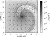 |
Fig. 1 Quasi-stationary density and velocity distribution resulting from a simulation with Ṁ = 2 × 10⁻⁶ M⊙ yr-1 and ν∞ = 20 km s-1 after ~1 orbit or ~2560 yrs. The dotted arrow indicates the line of sight to the B star, whose position is marked by the asterisk. The grey rectangles indicate the contours of the high-resolution subgrids (see text). |
2.3. Plasma simulations
The temperature and ionization inside the H ii region around the B star were calculated with version 08.00 of the plasma code Cloudy, last described by Ferland et al. (1998). Cloudy uses a spherical geometry in 1D. To obtain a 3D temperature distribution of the α Sco system we calculated different models, each one corresponding to a different direction, starting from the position of the source of ionizing radiation, i.e. the B star (see Appendix A for details). This approach is justified as Cloudy uses the escape probability formalism for the calculation of radiative transfer effects, so that different points inside the circumstellar envelope do not interact with each other. For the radiation of the B star we used a synthetic spectrum given by an interpolation on the TLUSTY grid of Lanz & Hubeny (2007).
The resulting temperature distribution is then passed to the hydro code as a source term affecting the total energy. The radiative heating is assumed to take place at a much smaller time scale than the hydrodynamic processes. This procedure is repeated at regular intervals during the calculation, typically every other time step as measured on the base grid. The information about the state of ionization can be used later in the analysis of spectral lines.
For the treatment of Fe ii, Cloudy provides a large model atom developed by Verner et al. (1999). It includes the 371 lowest levels of the Fe+ ion, i.e., up to 93 487.65 cm-1.
3. Results
3.1. Density and velocity distribution
The presence of the hot H ii region inside the wind of the supergiant causes deviations from spherical symmetry. Figure 1 shows a cut through the center of mass of the system parallel to the plane of the orbit, including the density distribution as well as appropriately scaled velocity vectors for a simulation with Ṁ = 2 × 10⁻⁶ M⊙ yr-1 and ν∞ = 20 km s-1 after ~1 orbit or ~2560 yrs. At the boundaries of the H ii region around the B star that face the supergiant the density increases, and it decreases inside the wake of the H ii region. The curved shape of the structure results from the orbital motion. The orientation of the velocity vectors is still approximately spherically symmetric, but the absolute value increases by ~50% in the low-density regions. Figure 2 shows the central region of Fig. 1 including the H ii region as a contour that indicates 90% ionization of hydrogen.
We calculated models with different values of Ṁ (0.2, 0.5, 1, 2, and 5 × 10⁻⁶ M⊙ yr-1) and ν∞ (10, 20, and 40 km s-1), including all possible combinations of Ṁ and ν∞ in these ranges.
3.2. Comparison to observed circumstellar absorption lines
Circumstellar absorption lines in the spectrum of α Sco B have been observed with GHRS/HST (Baade & Reimers 2007) and with UVES/VLT (Reimers et al. 2008). In Sect. 3.2.1, we describe the calculation of synthetic line profiles based on the simulations presented above. These synthetic profiles are compared to observations in Sect. 3.2.3. For that comparison, we calibrated the wavelength scale of the GHRS spectra by use of the UVES spectra (see Sect. 3.2.2). It should be noted that the resonance lines (0 eV) of abundant ions are affected by interstellar contamination, as shown by Hagen et al. (1987). Exceptions are those elements which are heavily depleted in the IS medium.
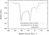 |
Fig. 3 Calculations of the Zn ii UV mult. 1 2062.660 Å absorption line based on a hydrodynamic simulation including ionization with Ṁ = 10-6 M⊙ yr-1 and ν∞ = 20 km s-1, and on an undisturbed, spherically expanding wind. As a convergence test, the hydrodynamic results (low resolution) are compared to a model with the same parameters but with a resolution that is increased by a factor of two (high resolution). The difference in the component at ~−29 km s-1 is due to the reduced size of the computational domain in the high-resolution simulation (see text). The abscissa gives the radial velocity relative to the center of mass of the system. |
3.2.1. Synthetic line profiles
To derive the profiles of circumstellar lines we use the density and velocity information from the hydrodynamic simulations to calculate a pure absorption line profile given by  (4)where Iν is the emergent intensity, IB the intensity of the B star continuum, χν the opacity, and z the coordinate along the line of sight towards the B star, which is located at z = zB. zmax is chosen so large that the line profile does not change if a higher value is used for this limit. After about one half of an orbit the density structure becomes quasi-stationary and does not change its shape anymore. Therefore, the results from the hydrodynamic simulations at any time step can be used for the calculation of the line profile. We used the density information corresponding to the time after about one orbit, i.e. at t ~ P, where P ~ 2560 yrs is the orbital period of the system.
The resulting profiles deviate considerably from the profiles resulting from a continuous, spherically symmetric model. As an example, Fig. 3 shows the simulated profile of the Zn ii UV mult. 1 2062.660 Å absorption line, based on a simulation with Ṁ = 10-6 M⊙ yr-1 and ν∞ = 20 km s-1, along with a plot of the same line for the case of an undisturbed, spherically expanding wind with the same parameters. Obviously, the absorption component at ~−20 km s-1 is present in both lines and coincides with the terminal wind velocity, but the absorption profile that is based on the hydrodynamic simulation exhibits a more complex structure, which finds expression in three additional minima, namely at ~−29, −7, and 3 km s-1. The radial velocities are measured relative to the center of mass of the system. Thermal broadening is included by applying a constant temperature of 5000 K, which is approximately the mean temperature inside the H ii region. Microturbulence is not included in the calculation of the line profiles, so that all additional effects that influence the line profile are of hydrodynamic origin.
The distinct components seen in the absorption line presented in Fig. 3 are related to features of the density and velocity distribution along the line of sight to the B star. Figure 4 shows the number density of Zn+ and the radial velocity as a function of distance to the B star. One important result is that the velocity is no longer a monotonic function of distance when hydrodynamic effects are included, but there is a broad minimum around ~4000 AU.
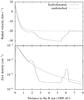 |
Fig. 4 Radial velocity relative to the center of mass and Zn ii number density along the line of sight to the B star, based on a hydrodynamic simulation and on an undisturbed, spherically expanding wind. These data correspond to the absorption line profiles shown in Fig. 3 (Ṁ = 10-6 M⊙ yr-1, ν∞ = 20 km s-1). |
To test whether the simulations have converged, we calculated an additional line profile based on a simulation with the same parameters, but with a resolution that is enhanced by a factor of two (see Fig. 3). The result does not show any significant changes. For this high-resolution simulation we used a computational domain with a reduced size of ax × ay × az ~ 6217 × 6217 × 3419 AU, because it would have been computationally too expensive to calculate a high-resolution model of the same size as the low-resolution models. This reduced computational domain does not cover the whole high-velocity region that produces the absorption component at ~−29 km s-1. That means that the broad minimum in the radial velocity (Fig. 4) is not fully covered, which results in a weaker absorption component.
Figure 5 shows the dependence of the Zn ii UV mult. 1 2062.660 Å and Cr ii UV mult. 1 2062.236 Å lines on the mass-loss rate. While the position of the component at ~−20 km s-1 remains nearly unchanged, the position of the other strong component, which is associated to the increased density at the boundary of the H ii region, shifts to lower velocities as the mass-loss rate decreases and the H ii region becomes more extended. There is also a component at ~−29 km s-1, which is very weak in the Zn ii line. The profiles of the Cr ii line show that this component is considerably stronger at lower mass-loss rates. This is because the wake of the H ii region is more extended if the overall density is lower, so that the minimum of the radial velocity, shown in Fig. 4 for Ṁ = 10-6 M⊙ yr-1, becomes broader and a higher number of particles along the line of sight move with velocities larger than the terminal wind velocity ν∞. That is, the larger extent of the volume containing gas at high velocities, which produces the absorption component at − 29 km s-1, overcompensates the effect of the decreased density.
In the Cr ii line there is practically no absorption at positive velocities, because most chromium is doubly ionized throughout the H ii region. In contrast, Zn++ is only present close to the B star, which is partly due to the different ionization potentials of Zn+ (144 893 cm-1) and Cr+ (132 966 cm-1). The relative abundances of H+, Cr+, and Zn+ are shown in Fig. 6 as a function of distance to the B star along the line of sight.
3.2.2. Calibration of the observed wavelength scale
The positions of the observed absorption components in the GHRS spectra are slightly different in every line (Baade & Reimers 2007), which is due to the relatively large error of the wavelength calibration. The data were recorded using the Large Science Aperture of GHRS, which results in a maximum error of ~4.5 km s-1 (Heap et al. 1995). The wavelength calibration of the spectra observed with UVES is much more accurate. It amounts to ≳ 120 m s-1 (D’Odorico et al. 2000). The panel at the top right of Fig. 7 shows the Ca ii mult. 1 (H and K) lines. There are three components in both lines, at − 21.0, − 13.6, and − 5.9 km s-1, respectively.
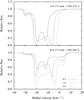 |
Fig. 5 Absorption profiles of the Zn ii UV mult. 1 2062.660 Å and Cr ii UV mult. 1 2062.236 Å lines for different mass-loss rates (ν∞ = 20 km s-1). The mass-loss rates are given at the bottom right of the figure in units of 10-6 M⊙ yr-1. |
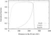 |
Fig. 6 Ionization fractions of different ions as a function of distance to the B star along the line of sight. The data are derived from a simulation using Ṁ = 10-6 M⊙ yr-1 and ν∞ = 20 km s-1. |
Now, supposing that the component at −21 km s-1 in the Ca ii lines is associated to the terminal wind velocity as suggested by the synthetic line profiles presented in the previous section, the positions of the GHRS lines can be calibrated by applying shifts that place the most blue-shifted strong component at − 21 km s-1, which is acceptable as long as the shifts are smaller than the maximum error of the GHRS wavelength calibration (4.5 km s-1). Table 2 lists the shifts corresponding to the five GHRS lines presented in Fig. 7. The Cr ii line is saturated, so that the positions of the strong absorption components are rather uncertain. Therefore, the shift determined for the Zn ii line is used, which lies very close to the Cr ii line. For the Fe ii line the central component is used to define the shift, because the observed component near −21 km s-1 is weak and not clearly pronounced.
Observed absorption lines of Ti ii also show a strong absorption component at ~−21 km s-1, which may serve as an additional justification for identifying the position of this component with the terminal wind velocity. The two panels at the bottom right of Fig. 7 show absorption line profiles of the Ti ii multiplets 1 and 2.
3.2.3. Observed line profiles
Figure 7 shows a selection of absorption lines observed with GHRS/HST and UVES/VLT in the spectrum of α Sco B. The shapes of the line profiles produced by different ions or different energy levels of the same ion (Ti ii) show a large variety. The observed absorption features depend on the excitation of fine-structure levels of the ions and the ionization of the corresponding element along the line of sight. Most of the lines exhibit three strong absorption components at the approximate positions −21, −14, and −6 km s-1, respectively. Some of the lines produced by the 0 eV levels have an additional component at − 29 km s-1 (Ti ii 3383.759 Å, Cr ii 2062.236 Å, Zn ii 2062.660 Å, and Ni ii 1393.324 Å), which can be explained by the broad minimum of the radial velocity in the wake of the H ii region far from the B star (see Figs. 5 and 4).
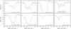 |
Fig. 7 Absorption profiles observed in the spectrum of α Sco B with HST/GHRS (Cu ii, Fe ii, Ni ii, Zn ii, and Cr ii lines) and VLT/UVES (Ti ii and Ca ii lines). |
For the comparison presented in the following, a systemic velocity of νsys = −1.3 km s-1 is added to the wavelength scale of the simulated profiles, which results from a comparison of the projected orbital velocities resulting from the adopted orbital configuration (δ = 23°, e = 0) with the observed radial velocities (see Reimers et al. 2008).
Cr ii, Cu ii, Ni ii, and Zn ii.
Figure 8 shows a comparison of the observed Cr ii, Cu ii, Ni ii, and Zn ii lines presented in Fig. 7 to theoretical profiles corresponding to a mass-loss rate of Ṁ = 2 × 10⁻⁶ M⊙ yr-1 and a wind velocity of ν∞ = 20 km s-1. The simulated line profiles are convolved with a Gaussian profile function with a FWHM of 3.5 km s-1 to account for the limited resolution of the GHRS/HST spectra.
 |
Fig. 8 Comparison of theoretical line profiles (solid curves) corresponding to a mass-loss rate of Ṁ = 2 × 10⁻⁶ M⊙ yr-1 and a wind velocity of ν∞ = 20 km s-1 with observations (dashed curves), including a velocity calibration provided by the UVES spectra (see Sect. 3.2.2) and a systemic velocity of −1.3 km s-1. The relative flux is given as a function of the observed radial velocity. |
Obviously, there are a number of differences between the simulated and the observed line profiles. First of all, there are only two strong components in the simulated profiles, whereas there are three in the observed profiles. Secondly, the observed component at −6 km s-1 is much stronger than predicted by the model calculations in the Zn ii and Cu ii lines. However, with the wavelength calibration described in Sect. 3.2.2 the positions of the two strong components in the simulated profiles approximately match the positions of the outer two of the observed strong components. It turns out that, within the error of the wavelength calibration, the observed GHRS profiles are consistent with the assumption that the position of the most blue-shifted of the strong absorption components is at −21 km s-1, as suggested by the absorption lines measured with UVES and by the theoretical lines, all of which include a strong absorption component at the position corresponding to the terminal wind velocity.
The weaker absorption component at ~−29 km s-1, which is clearly visible in the Cr ii and the Zn ii line, is very weak in the corresponding theoretical profiles. The simulations predict a stronger absorption component at this position for lower mass-loss rates, especially in the Cr ii line (see Fig. 5). This may be an indication of a time-dependent mass-loss rate, which could produce distinct absorption components corresponding to different mass-loss rates (see Sect. 4.2).
The equivalent widths of the observed profiles and the simulated profiles shown in Fig. 8 agree well. Moreover, the component at ~−21 km s-1 of the simulated profiles gives a good fit of the observed components. The absorption in the components at −6 km s-1 is stronger in the observed lines, which may be due to interstellar absorption as all the lines result from transitions starting from the lowest energy levels of the ions. The theoretical absorption lines resulting from simulations using a mass-loss rate of Ṁ = 10-6 M⊙ yr-1, as given by Reimers et al. (2008) based on a simplified model of the circumstellar shell neglecting dynamic effects, are much weaker than the observed ones. That shows the significant impact of the hydrodynamic effects, which will have to be considered in future studies of mass loss.
Differences between the observed and simulated profiles are to be expected, because the simulations do not account for a possible time dependence of the mass-loss rate. Indications of multiple shell ejection have been observed in IR images in both α Sco and α Ori (e.g. Danchi et al. 1994, see also Sect. 1). The additional third component in the observed lines seen in Fig. 8 at ~−14 km s-1 could well be the result of such a discrete ejection. An additional complication of a comparison of observations with theory is the observed differential depletion (Baade & Reimers 2007). These effects may be the reason for a more complicated structure of the absorption profiles.
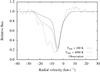 |
Fig. 9 Observed and theoretical absorption profiles of the Fe ii UV mult. 1 2622.452 Å line for Ṁ = 2 × 10⁻⁶ M⊙ yr-1 and ν∞ = 20 km s-1. For the theoretical profiles, two different lower limits of the electron temperature were used in the corresponding plasma simulations (see text). The relative flux is given as a function of the observed radial velocity. |
Fe ii.
The observed absorption profile of the Fe ii UV mult. 1 2622.452 Å line presented in Fig. 7 results from the fine structure level in the ground term at 977.053 cm-1. The population of this level cannot be reproduced by applying a constant scale factor to the total Fe+ density, as would be expected if the levels were populated according to their statistical weights.
The model atom of Verner et al. (1999) that was used in the plasma simulations yields the population of the level at 977.053 cm-1, which is the highest level in the ground term. It turns out that the relative population of the level is very low inside the cool neutral wind. The population of the Fe ii energy levels depends on the electron temperature, which determines the rate of collisions. The temperature inside the H ii region is ~5000 K, but the temperature in the H i region is not exactly known.
Figure 9 shows the absorption line profiles corresponding to two different lower limits of the electron temperature along with the observed absorption profile, which is shifted by − 1.6 km s-1 according to Table 2 (cf. Sect. 3.2.2). In these simulations, the temperature was not allowed to fall below a given lower limit. Obviously, the relative population of the 977.053 cm-1 level steeply decreases after a peak at the boundary of the H ii region. The slope of the right flank of the strong absorption components in the theoretical profiles does not exactly match the observed one, because there is a considerable amount of reemission, which is not included in the calculation of the theoretical line profiles. The decrease of the absorption towards lower velocities qualitatively matches the observation, although the slope is much too steep in the theoretical profiles. The absence of the middle absorption component in the theoretical profiles is not surprising since it is absent in all theoretical profiles (cf. Sect. 3.2.1).
The assumption that the neutral part of the wind has a temperature of 4000 K is probably not realistic, and even in this case the predicted absorption is too weak in the outer parts of the envelope. A value of T ≲ 1000 K in the H i region is more realistic. Apparently the calculation of the level population with Cloudy does not give correct results, maybe because of an underestimation of the rates of collisional or radiative processes that populate the level that is responsible for the absorption, or because of advection effects, which are not included in the simulations (see Sect. 4). In the plasma simulations, the gas is assumed to be at rest with respect to the B star, which may introduce another uncertainty in the calculation of the populations of fine-structure levels, as the velocity field may have considerable effects on the continuum pumping rates. However, the strength of the absorption component at ~−6 km s-1 approximately matches the strength of the observed component, so that the mass-loss rate of 2 × 10⁻⁶ M⊙ yr-1, which is consistent with the observed profiles of the lines of other ions (cf. Fig. 8), can be confirmed.
The results presented in this section suggest that the weakness of the observed absorption components of this Fe ii line at − 14 and − 21 km s-1 is due to the relatively high energy difference between the lowest level and the fine-structure level corresponding to the transition. Apparently the mechanisms that excite Fe ii to higher fine-structure levels are not efficient in the outer parts of the circumstellar envelope, i.e. at low densities, far from the B star and its H ii region.
Ca ii and Ti ii.
The number densities of Ca+ and Ti+ along the line of sight cannot be reproduced in the framework of the present model. In the case of Ti+, the plasma simulations yield a density that is much too high and density gradients that are too steep to reproduce the observed absorption profiles. The ionization of Ti+ is complicated because its ionization potential (13.576 eV) is close to the Lyman edge. Simulations show that the ionization of Ti+ sensitively depends on the local temperature in the circumstellar shell. The absence of the absorption components at −6 and −14 km s-1 in the observed line profiles of Ti ii shown in Fig. 7 suggests that most titanium is at least doubly ionized up to a large distance to the B star, i.e. even far outside the H ii region. However, the absence of these components may also be due to dust depletion. The component at − 30 km s-1 is observed only in the 0 eV transitions of Ti ii, which supports evidence from the simulations that the line is formed far away from the system. In the case of Ca+, the predicted number density is much too low. In the whole circumstellar envelope Ca++ appears to be the dominant stage of ionization of calcium, and Ca+ shows a very complex dependence on the varying conditions along the line of sight. Thus, the Ca ii lines are inappropriate for mass-loss diagnostics.
The simplified treatment of the corresponding model atoms may be the reason for the discrepancy between theory and observation in the case of Ca ii and Ti ii. The Cloudy code treats Ca+ as a five-level atom, which includes the fine-structure levels of only the lowest three terms (4s, 3d, and 4p) with the corresponding transitions (multiplets 1, 2, and 1F). Ti+ is treated in the framework of the scandium-like isoelectronic sequence as a five-level atom without resolving any fine-structure components, including only the terms a4F, z , z
, z , and the terms and
  of the configuration 3d(2D)4s4p(
 ). Thus, for Ti+, populations of individual fine-structure levels are not calculated. Moreover, only transitions to the ground term of Ti ii are included in the simulation. The depletion of titanium due to dust formation is probably the most significant effect producing deviations from the observed data (cf. Baade & Reimers 2007).
3.3. Comparison to optical line emission from the Antares nebula
The Antares emission nebula, which is associated to the H ii region around α Sco B, is seen in the optical in Hα and various other emission lines, last described in detail by Reimers et al. (2008). The simulations presented above will be compared to observations of the Hα emission in Sect. 3.3.1. Moreover, forbidden transitions of Fe ii, which produce the most prominent emission lines of the Antares nebula, will be used to compare observations to our model in Sect. 3.3.2. The observations were performed with UVES/VLT using a long slit perpendicular to the line connecting the two stars, and yielded a scan of the emission nebula with a step size of  , starting 09 west of the supergiant (see Fig. 10).
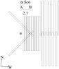 |
Fig. 10 Slit positions used for the observations of the Antares nebula. The rectangles indicate the position and size of the slit in the blue arm relative to the α Sco system as it is seen in the sky. This is Fig. 1 from Reimers et al. (2008). |
3.3.1. Hα emission
The plasma simulations show that the strongest Hα emission in the Antares nebula emerges near the B star, where most hydrogen is ionized. Outside the H ii region the emission is much weaker and follows the total density (Fig. 1). In an H ii region, Hα is naturally produced by recombination of electrons and protons. Another important mechanism is pumping by Lyman line photons from the source of radiation, so that the presence of Lyman absorption or emission lines in the spectrum of the source of radiation affects the production of Hα photons. The B-star atmospheres presented in the TLUSTY grid (Lanz & Hubeny 2007) show strong absorption in the Lyman lines. As the Antares H ii region is optically thin in Hα, the observed emission is solely determined by the population of the upper levels and the oscillator strengths. The sensitivity of the Hα emission produced in the H ii region to changes of the input flux in the range of the Lyman lines requires a high-resolution input spectrum in the Cloudy simulations. For the calculations presented in this section we used a resolution of Δν/ν = 5 × 10⁻⁴.
The spatial extent of the H ii region is determined by the mass-loss rate of the supergiant and the Lyman-continuum flux of the B star, and can be measured by observing the spatial extent of the Hα emission from the Antares nebula (cf. Reimers et al. 2008). Figure 11 shows the Hα intensity distribution at 34 from the supergiant, measured on the projected line connecting the two stars (see Fig. 10). The shape and extent of the observed and theoretical Hα intensity distributions agree, but the center of the theoretical distribution is shifted to higher velocities with respect to the observed distribution. This is probably due to the uncertainties in the geometry of the system and can be explained by an overestimation of the position angle of the line connecting the two stars relative to the plane of the sky (e = 0 is only a rough estimate, and due to the long period it will be difficult to improve on this).
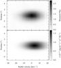 |
Fig. 11 Hα emission at 3 |
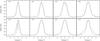 |
Fig. 12 Frequency-integrated Hα flux as a function of position along the slit for a simulation with Ṁ = 2 × 10⁻⁶ M⊙ yr-1 and ν∞ = 20 km s-1 (solid lines), and the corresponding observations (dashed lines). |
The intensity in Fig. 11 is given as a function of velocity. Assuming pure emission, the emergent intensity is given by the integral ![Mathematical equation: \begin{equation} I_{\varv}(\varv) = \int_{s_{\min}}^{s_{\max}}j(s)\Phi\left[\varv_{r}(s) - \varv\right]\mathrm{d}s, \end{equation}](/articles/aa/full_html/2012/10/aa19659-12/aa19659-12-eq123.png) (5)where s ranges from smin = −0.3a to smax = + 0.3a along the line of sight, and the zero point lies in the plane defined by the line connecting the two stars and the direction perpendicular to the orbit, so that the H ii region is fully included. a is the edge length of the domain in x and y direction. smin and smax were chosen such that the integration includes a maximum of the available simulated data but does not exceed the boundaries of the computational domain at the outermost slit position. As most of the Hα emission comes from the H ii region, this range ensures that the integration covers the whole emitting region. j is the emission coefficient for isotropic emission,
(5)where s ranges from smin = −0.3a to smax = + 0.3a along the line of sight, and the zero point lies in the plane defined by the line connecting the two stars and the direction perpendicular to the orbit, so that the H ii region is fully included. a is the edge length of the domain in x and y direction. smin and smax were chosen such that the integration includes a maximum of the available simulated data but does not exceed the boundaries of the computational domain at the outermost slit position. As most of the Hα emission comes from the H ii region, this range ensures that the integration covers the whole emitting region. j is the emission coefficient for isotropic emission, 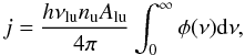 (6)resulting from the frequency νlu of the transition, the number density nu of ions in the upper state, the transition probability Alu, and the profile function φ(ν). h is Planck’s constant, νr(s) the radial velocity at s, and Φ a Gaussian profile that introduces thermal broadening,
 ![Mathematical equation: \begin{equation} \Phi(\varv) = \frac{1}{\Delta\varv_\mathrm{D}\sqrt{\pi}} \exp{\left[-\frac{\varv^2}{\left(\Delta\varv_\mathrm{D}\right)^2}\right]}, \end{equation}](/articles/aa/full_html/2012/10/aa19659-12/aa19659-12-eq139.png) (7)where the Doppler width ΔνD is defined by pure thermal broadening with a temperature of 5000 K. Microturbulent broadening is not included, so that the hydrodynamic effects can be clearly identified. is the intensity per unit radial velocity, and the intensity per unit frequency reads , where λ0 is the rest wavelength of the transition.
(7)where the Doppler width ΔνD is defined by pure thermal broadening with a temperature of 5000 K. Microturbulent broadening is not included, so that the hydrodynamic effects can be clearly identified. is the intensity per unit radial velocity, and the intensity per unit frequency reads , where λ0 is the rest wavelength of the transition.
For a comparison with the observations as presented in Fig. 11 for Hα, the spectral resolution of UVES and the seeing have to be considered. An analysis of the lines of the wavelength calibration lamp yields an average FWHM of 3.5 km s-1 in the vicinity of the [Fe ii] mult. 20F 4814.55 Å line, which we present in the next section, in the range from 4789 to 4832 Å. We adopt this value for the spectral resolution of the UVES spectra. The seeing during the observations was  . Therefore, the theoretical intensity distributions are convolved with a Gaussian profile of FWHM = 3.5 km s-1 along the frequency coordinate and with another Gaussian corresponding to the seeing in the direction of the spatial coordinate along the slit. A systemic velocity of − 1.3 km s-1 is added to the theoretical velocity scale (see Sect. 3.2.3).
For a comparison of the spatial extent of the observed and theoretical emission, it is easier to compare the frequency-integrated emission as a function of position along the slit. The integration of the theoretical data reads  (8)The results are shown for different slit positions in Fig. 12 for a simulation with Ṁ = 2 × 10⁻⁶ M⊙ yr-1 and ν∞ = 20 km s-1, along with the corresponding observational data. In this simulation, the slit skims only the outermost part of the H ii region at the slit positions 19 and 54. Therefore, the theoretical data at these slit positions should be interpreted with care, because outside the H ii region the Hα production is dominated by line pumping effects, which may not be well reproduced with the simplified approach used by Cloudy for the radiative transfer (see Sect. 2.3). The central minimum in the observations corresponding to 24 is probably due to an artifact related to the data reduction. At the other slit positions, the simulated and observed distributions agree well in shape and extent.
At 24 and 29, the theoretical Hα profiles are narrower than the observed profiles, indicating a lower mass-loss rate, while the observed data at the other slit positions further away from the supergiant are better reproduced by the model. This may be due to the mass loss rate being time-dependent.
3.3.2. [Fe ii] emission
The most prominent emission lines seen in the Antares nebula are the forbidden iron lines. The spatial and spectral distribution of the line at 4814.55 Å (multiplet F20) was presented in detail by Reimers et al. (2008). The data obtained with the Cloudy calculations, which include the large Fe+ model atom of Verner et al. (1999) (see Sect. 2.3), can be used to compare the results of the simulations to the observed data.
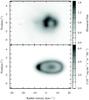 |
Fig. 13 [Fe ii] mult. 20F 4814.55 Å emission at 3 |
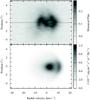 |
Fig. 14 [Fe ii] mult. 20F 4814.55 Å emission at 5 |
As an example, Fig. 13 shows the distribution of the [Fe ii] mult. 20F 4814.55 Å intensity at 34 both for the observed and the simulated data. Obviously, the simulations do not yield a realistic picture of the [Fe ii] emission for that slit position. The simulations suggest a circular structure around a central maximum at ~5 km s-1, while the maximum flux in the observed data is concentrated in a more compact structure, which is approximately circular but open to the bottom, between ~0 and ~8 km s-1 as measured at the center of the slit. The overall extent of the observed emission approximately agrees with the theoretical distribution and is consistent with the extent of the Hα emission in both the velocity and the spatial coordinate.
The discrepancies between the observed and theoretical [Fe ii] emission could be due to an inadequate treatment of the Fe+ ion in the Cloudy code. The emission may also be influenced by advection effects, which may be significant especially at the western boundary of the H ii region towards the open side of the wake, where the density is small. An alternative explanation would be that due to dust depletion in the high density boundaries of the structure, a large fraction of Fe is not available for Fe ii emission. This effect seems to increase with distance to the B star.
A common feature of the observed forbidden and allowed Fe+ emission is an asymmetry with respect to the center of the slit, which is clearly visible e.g. at 54 from the supergiant (Fig. 14). Apparently, there is more emission from the northern than from the southern half (see also Fig. 13). This is another indication of density structures that are not included in the model, which is symmetric with respect to the plane of the orbit. A deviation of the inclination from 90° would also cause such an asymmetry. However, the Hα flux distributions do not show any significant asymmetries.
4. Discussion
4.1. The mass-loss rate
The hydrodynamic simulations presented in Sect. 3.1 show that the hot H ii region that is moving with the B star through the circumstellar envelope of α Sco produces strong deviations from spherical symmetry in the density and velocity distributions. The theoretical absorption line profiles derived from these simulations (Sect. 3.2.1) exhibit a pronounced multi-component structure comparable to the observed line profiles presented in Fig. 7. The best match between theoretical and observed line profiles is achieved with a mass-loss rate of Ṁ = 2 × 10⁻⁶ M⊙ yr-1 and a wind velocity of ν∞ = 20 km s-1 (Sect. 3.2.3). This value of the mass-loss rate is twice as high as the rate derived by Reimers et al. (2008), which was based on a spherically expanding model of the circumstellar shell. This discrepancy is due to the decreased density in the wake of the H ii region (see Figs. 1 and 2).
The range of values of Ṁ and ν∞ that is covered by the simulations is rather small, owing to the limitations imposed by the large amount of computing time that the hydro code requires. As the AMRCART code is not adapted to modern parallel computing clusters, the hydrodynamic simulations were carried out on a single CPU core, while only the photoionization/radiative-transfer calculations were executed in parallel. A finer grid in Ṁ and ν∞ would improve the accuracy of the resulting mass-loss rate, and it might be instructive to calculate models with different semi-major axes and position angles to account for the uncertainties in the orbital parameters (see next section). However, the theoretical data presented in this work and the available observations agree fairly well, and the remaining systematic errors (see below) are probably larger than the error that is due to the coarseness of the grid of models, i.e. the relatively large step size in Ṁ and ν∞. We presume that the total error of the mass-loss rate including systematic uncertainties is ~5 × 10⁻⁷ M⊙ yr-1.
An important systematic error is introduced by the observed differential dust depletion (Baade & Reimers 2007). This effect depends on the considered element and on the local conditions in the circumstellar shell. It results in the observed absorption profiles being weaker than predicted for a given mass-loss rate. In contrast, interstellar absorption can make the absorption components near 0 km s-1 stronger than predicted by the model, which is probably responsible for the discrepancies in the Zn ii 2062.660 Å and Cu ii 1358.773 Å lines (Fig. 8). According to Snow et al. (1987) and Cardelli (1984), dust depletion is of minor importance for zinc, which means that the mass-loss rate can best be determined by use of the Zn ii absorption lines.
In the present approach, the radiative transfer is treated in a simplified manner with the escape probability formalism (cf. Sect. 2.3). This is probably the major source of error in the calculation of the [Fe ii] line emission, and the exact solution of the scattering problem would probably resolve some of the apparent discrepancies between the theoretical predictions and the observations. Moreover, some of the circumstellar absorption lines in the spectrum of α Sco B, e.g. Cr ii 2062.236 Å, have P Cyg-type profiles, which cannot be reproduced with a pure absorption model. For a calculation of the reemission that is superposed in these lines on the absorption profile, exact radiative transfer simulations have to be included in the model.
4.2. Asymmetries and time-dependent effects
The observations indicate an asymmetric, non-stationary character of the circumstellar shell of α Sco. The observed absorption lines exhibit an additional component at − 14 km s-1, which cannot be reproduced with the assumption of a constant mass-loss rate. Moreover, the integrated Hα flux (Fig. 12) also appears to indicate slightly different mass-loss rates at different distances to the B star (Sect. 3.3.1). The observations of [Fe ii] emission reveal that the density distribution is not symmetric with respect to the plane of the orbit, which cannot be reproduced in the framework of the present model.
The uncertainties in the geometry of the α Sco system may partly account for the asymmetry of the observed [Fe ii] emission and the shift of the theoretical emission in Hα and [Fe ii] 4814.55 Å. The orbital parameters, such as the inclination, eccentricity, and the orbital velocities, are not well known because of the large orbital period (~2560 yrs). Especially the radial velocity of the supergiant is hard to measure, because the observed velocity results from a superposition of pulsations and orbital motion (Smith et al. 1989).
The plasma calculations used for determining the temperature and ionization structure of the circumstellar envelope are based on the assumption that the time scales of cooling and heating are small compared to the dynamic time-scale. This is not exact at the western boundary of the H ii region, towards the low-density wake, where also advection effects may have a significant impact on the ionization balance. A model including time-dependent plasma-effects may considerably improve the understanding of the observed absorption and emission features and could be the subject of future studies.
5. Conclusions and outlook
The results of the combination of observations with hydrodynamic and plasma simulations presented in this work show that the circumstellar envelope of the α Sco system is strongly influenced by dynamic effects. A calculation of absorption line profiles based on the simulated density and velocity distributions and ionization structure, and a comparison to GHRS/HST and UVES/VLT spectra reveal that the mass-loss rate was underestimated by a factor of two in earlier studies that were based on an undisturbed, spherically symmetric circumstellar shell. The resulting mass-loss rate of Ṁ = 2 × 10⁻⁶ M⊙ yr-1 is confirmed by an analysis of the Hα emission from the Antares nebula, which is based on spatially resolved emission distributions observed with UVES.
The theoretical absorption line profiles exhibit a multi-component structure as a natural result of the influence of the hot H ii region that is moving with the B star through the wind of the primary. Three of the four observed components can be explained accordingly. However, the origin of the additional component at − 14 km s-1 seen in most absorption lines (Fig. 7) remains uncertain and is probably an indication of time-dependent mass-loss.
The structure of the [Fe ii] line emission of the Antares nebula as observed with UVES cannot be reproduced correctly. A more sophisticated model including exact radiative transfer calculations and time-dependent simulations of the ionization balance allowing for advection effects would help to understand the remaining discrepancies between theory and observations. In this context, it would be desirable to parallelize the hydro code, which will make it possible to calculate a more extensive grid of models. Future projects may deal with these improvements of the model calculations.
A number of empirical mass-loss rates of ζ Aur systems were determined on the basis of spherically symmetric density and velocity distributions (see e.g. Che et al. 1983; Baade et al. 1996). Some of these systems, e.g. ζ Aur and 31 Cyg, also contain H ii regions, which may lead to even more severe dynamic effects than in α Sco due to the much smaller orbital periods. The current values of the mass-loss rates of these stars may have to be revised on the basis of more realistic models including dynamic processes as presented in this work for α Sco.
Acknowledgments
K.B. gratefully acknowledges support by a fellowship from the Landesgraduiertenförderung Hamburg.
References
- Baade, R. 1998, in Ultraviolet Astrophysics Beyond the IUE Final Archive, eds. W. Wamsteker, R. G. Riestra, & B. Harris, ESA Sp. Publ., 413, 325 [Google Scholar]
- Baade, R., & Reimers, D. 2007, A&A, 474, 229 [NASA ADS] [CrossRef] [EDP Sciences] [Google Scholar]
- Baade, R., Kirsch, T., Reimers, D., et al. 1996, ApJ, 466, 979 [NASA ADS] [CrossRef] [Google Scholar]
- Barmin, A. A., Kulikovskiy, A. G., & Pogorelov, N. V. 1996, J. Comput. Phys., 126, 77 [NASA ADS] [CrossRef] [Google Scholar]
- Berger, M. J., & Colella, P. 1989, J. Comput. Phys., 82, 64 [NASA ADS] [CrossRef] [Google Scholar]
- Bressan, A., Fagotto, F., Bertelli, G., & Chiosi, C. 1993, A&AS, 100, 647 [NASA ADS] [Google Scholar]
- Brott, I., de Mink, S. E., Cantiello, M., et al. 2011, A&A, 530, A115 [NASA ADS] [CrossRef] [EDP Sciences] [Google Scholar]
- Cardelli, J. A. 1984, AJ, 89, 1825 [NASA ADS] [CrossRef] [Google Scholar]
- Che, A., Hempe, K., & Reimers, D. 1983, A&A, 126, 225 [NASA ADS] [Google Scholar]
- Danchi, W. C., Bester, M., Degiacomi, C. G., Greenhill, L. J., & Townes, C. H. 1994, AJ, 107, 1469 [NASA ADS] [CrossRef] [Google Scholar]
- D’Odorico, S., Cristiani, S., Dekker, H., et al. 2000, in Discoveries and Research Prospects from 8- to 10-Meter-Class Telescopes, ed. J. Bergeron, SPIE Conf. Ser., 4005, 121 [Google Scholar]
- Ferland, G. J., Korista, K. T., Verner, D. A., et al. 1998, PASP, 110, 761 [Google Scholar]
- Hack, M., & Stickland, D. 1987, in Exploring the Universe with the IUE Satellite, ed. Y. Kondo et al. (Dordrecht: D. Reidel), Astrophys. Space Sci. Lib., 129, 445 [Google Scholar]
- Hagen, H.-J., Hempe, K., & Reimers, D. 1987, A&A, 184, 256 [NASA ADS] [Google Scholar]
- Heap, S. R., Brandt, J. C., Randall, C. E., et al. 1995, PASP, 107, 871 [NASA ADS] [CrossRef] [Google Scholar]
- Hjellming, R. M., & Newell, R. T. 1983, ApJ, 275, 704 [NASA ADS] [CrossRef] [Google Scholar]
- Hopmann, J. 1958, Mitteilungen der Universitätssternwarte Wien, 9, 135 [Google Scholar]
- Kudritzki, R. P., & Reimers, D. 1978, A&A, 70, 227 [NASA ADS] [Google Scholar]
- Lafon, J.-P. J., & Berruyer, N. 1991, A&ARv, 2, 249 [NASA ADS] [CrossRef] [Google Scholar]
- Lanz, T., & Hubeny, I. 2007, ApJS, 169, 83 [CrossRef] [Google Scholar]
- Marsh, K. A., Bloemhof, E. E., Koerner, D. W., & Ressler, M. E. 2001, ApJ, 548, 861 [NASA ADS] [CrossRef] [Google Scholar]
- Reimers, D. 1987, in Solar and Stellar Physics. Proceedings of the 5th European Solar Meeting, eds. E.-H. Schröter, & M. Schüssler (Berlin: Springer), Lect. Notes Phys., 292, 139 [Google Scholar]
- Reimers, D., Hagen, H.-J., Baade, R., & Braun, K. 2008, A&A, 491, 229 [NASA ADS] [CrossRef] [EDP Sciences] [Google Scholar]
- Smith, M. A., Patten, B. M., & Goldberg, L. 1989, AJ, 98, 2233 [NASA ADS] [CrossRef] [Google Scholar]
- Snow, Jr., T. P., Buss, Jr., R. H., Gilra, D. P., & Swings, J. P. 1987, ApJ, 321, 921 [NASA ADS] [CrossRef] [Google Scholar]
- Tuthill, P. G., Haniff, C. A., & Baldwin, J. E. 1997, MNRAS, 285, 529 [NASA ADS] [Google Scholar]
- Verner, E. M., Verner, D. A., Korista, K. T., et al. 1999, ApJS, 120, 101 [NASA ADS] [CrossRef] [Google Scholar]
- Walder, R., & Folini, D. 2000, in Thermal and Ionization Aspects of Flows from Hot Stars, eds. H. Lamers, & A. Sapar, ASP Conf. Ser., 204, 281 [Google Scholar]
- Willson, L. A. 2000, ARA&A, 38, 573 [NASA ADS] [CrossRef] [Google Scholar]
Appendix A: The temperature grid
For the calculation of the 3D temperature distribution, the 1D models calculated with Cloudy are distributed homogeneously in 3D space, i.e. with a constant increment in θ. The B star is the starting point for all 1D models, which give the physical conditions along a straight line in radial direction. The angle θ is measured from the upper pole, i.e. from the positive z direction in the AMRCART coordinate system, downwards, and the angle φ is measured counterclockwise from the direction towards the supergiant. The increment in φ in the plane of the orbit, i.e. at θ = π/2, equals the increment in θ, which is determined by a given number N according to Δθ = π/(N − 1). Only odd numbers are used for N so that there are always two models describing the temperature distribution on the line connecting the two stars, one away from the primary star, one towards it. In directions nearer to the poles, Δφ is increased according to Δφ = π/(Nsinθ − 1), where the expression Nsinθ is rounded to the nearest integer that is ≥ 2. For θ = 0 and θ = π one direction (φ = 0) is calculated.
Thus, the total number of Cloudy simulations computed to cover the whole domain for a given N is  (A.1)where 2(Ni − 1) is the number of directions calculated for a given θi = iΔθ, and
  (A.2)As the Cloudy simulations are independent of each other, they can be safely executed on different CPUs. The simulations presented in this work are symmetric with respect to the orbital plane so that it is sufficient to cover only the lower half of the domain, i.e.
  (A.3)For most of the simulations presented in this work, we used N = 9, i.e.
  . The only exception is the high-resolution simulation (cf. Fig. 3), where N = 13 and
  .
.
All Tables
All Figures
|
Fig. 1 Quasi-stationary density and velocity distribution resulting from a simulation with Ṁ = 2 × 10⁻⁶ M⊙ yr-1 and ν∞ = 20 km s-1 after ~1 orbit or ~2560 yrs. The dotted arrow indicates the line of sight to the B star, whose position is marked by the asterisk. The grey rectangles indicate the contours of the high-resolution subgrids (see text). |
| In the text | |
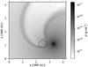 |
Fig. 2 Enlarged central region of Fig. 1. The contour indicates 90% ionization of hydrogen. |
| In the text | |
|
Fig. 3 Calculations of the Zn ii UV mult. 1 2062.660 Å absorption line based on a hydrodynamic simulation including ionization with Ṁ = 10-6 M⊙ yr-1 and ν∞ = 20 km s-1, and on an undisturbed, spherically expanding wind. As a convergence test, the hydrodynamic results (low resolution) are compared to a model with the same parameters but with a resolution that is increased by a factor of two (high resolution). The difference in the component at ~−29 km s-1 is due to the reduced size of the computational domain in the high-resolution simulation (see text). The abscissa gives the radial velocity relative to the center of mass of the system. |
| In the text | |
|
Fig. 4 Radial velocity relative to the center of mass and Zn ii number density along the line of sight to the B star, based on a hydrodynamic simulation and on an undisturbed, spherically expanding wind. These data correspond to the absorption line profiles shown in Fig. 3 (Ṁ = 10-6 M⊙ yr-1, ν∞ = 20 km s-1). |
| In the text | |
|
Fig. 5 Absorption profiles of the Zn ii UV mult. 1 2062.660 Å and Cr ii UV mult. 1 2062.236 Å lines for different mass-loss rates (ν∞ = 20 km s-1). The mass-loss rates are given at the bottom right of the figure in units of 10-6 M⊙ yr-1. |
| In the text | |
|
Fig. 6 Ionization fractions of different ions as a function of distance to the B star along the line of sight. The data are derived from a simulation using Ṁ = 10-6 M⊙ yr-1 and ν∞ = 20 km s-1. |
| In the text | |
|
Fig. 7 Absorption profiles observed in the spectrum of α Sco B with HST/GHRS (Cu ii, Fe ii, Ni ii, Zn ii, and Cr ii lines) and VLT/UVES (Ti ii and Ca ii lines). |
| In the text | |
|
Fig. 8 Comparison of theoretical line profiles (solid curves) corresponding to a mass-loss rate of Ṁ = 2 × 10⁻⁶ M⊙ yr-1 and a wind velocity of ν∞ = 20 km s-1 with observations (dashed curves), including a velocity calibration provided by the UVES spectra (see Sect. 3.2.2) and a systemic velocity of −1.3 km s-1. The relative flux is given as a function of the observed radial velocity. |
| In the text | |
|
Fig. 9 Observed and theoretical absorption profiles of the Fe ii UV mult. 1 2622.452 Å line for Ṁ = 2 × 10⁻⁶ M⊙ yr-1 and ν∞ = 20 km s-1. For the theoretical profiles, two different lower limits of the electron temperature were used in the corresponding plasma simulations (see text). The relative flux is given as a function of the observed radial velocity. |
| In the text | |
|
Fig. 10 Slit positions used for the observations of the Antares nebula. The rectangles indicate the position and size of the slit in the blue arm relative to the α Sco system as it is seen in the sky. This is Fig. 1 from Reimers et al. (2008). |
| In the text | |
|
Fig. 11 Hα emission at 3 |
| In the text | |
|
Fig. 12 Frequency-integrated Hα flux as a function of position along the slit for a simulation with Ṁ = 2 × 10⁻⁶ M⊙ yr-1 and ν∞ = 20 km s-1 (solid lines), and the corresponding observations (dashed lines). |
| In the text | |
|
Fig. 13 [Fe ii] mult. 20F 4814.55 Å emission at 3 |
| In the text | |
|
Fig. 14 [Fe ii] mult. 20F 4814.55 Å emission at 5 |
| In the text | |
Current usage metrics show cumulative count of Article Views (full-text article views including HTML views, PDF and ePub downloads, according to the available data) and Abstracts Views on Vision4Press platform.
Data correspond to usage on the plateform after 2015. The current usage metrics is available 48-96 hours after online publication and is updated daily on week days.
Initial download of the metrics may take a while.