| Issue |
A&A
Volume 546, October 2012
|
|
|---|---|---|
| Article Number | A23 | |
| Number of page(s) | 6 | |
| Section | The Sun | |
| DOI | https://doi.org/10.1051/0004-6361/201219268 | |
| Published online | 01 October 2012 | |
Cross helicity at the solar surface by simulations and observations
1
Leibniz-Institut für Astrophysik Potsdam,
An der Sternwarte 16,
14482
Potsdam,
Germany
e-mail: This email address is being protected from spambots. You need JavaScript enabled to view it.
; This email address is being protected from spambots. You need JavaScript enabled to view it.
2
Dept. of Astronomy,Stockholm University, Alba Nova University
Center, 10691
Stockholm,
Sweden
Received:
22
March
2012
Accepted:
24
July
2012
Abstract
A result of the quasilinear mean-field theory for driven magnetohydrodynamic (MHD) turbulence is that the observed cross helicity ⟨u·b⟩ may directly yield the magnetic eddy diffusivity ηT of the quiet Sun. In order to model the cross helicity at the solar surface, magnetoconvection under the presence of a vertical large-scale magnetic field is simulated with the nonlinear MHD code Nirvana. The very robust result of the calculations is that ⟨uzbz⟩ ≃ 2⟨u·b⟩ independent of the applied magnetic field amplitude. The correlation coefficient for the cross helicity is about 10%. Of similar robustness is the finding that the rms value of the magnetic perturbations exceeds the mean-field amplitude (only) by a factor of five. The characteristic helicity speed uη as the ratio of the eddy diffusivity and the density scale height for an isothermal sound velocity of 6.6 km s-1 prove to be 1 km s-1 for weak fields. This value coincides well with empirical results obtained from the data of the Hinode satellite and the Swedish 1-m Solar Telescope (SST) providing the cross-helicity component ⟨uzbz⟩. Both simulations and observations thus lead to the numerical value of ηT ≃ 1012 cm2/s as characteristic for the surface of the quiet Sun.
Key words: convection / magnetohydrodynamics (MHD) / Sun: granulation / Sun: surface magnetism
© ESO, 2012
1. Introduction
It is not easy to measure the turbulent magnetic diffusivity ηT
at the solar surface. This quantity determines the decay of magnetic structures with scales
larger than those of the turbulence. Theoretically, the decay of the magnetic structures
should depend on the relation of the magnetic field amplitude to the so-called equipartition
value  defined by the turbulence. This phenomenon is known as the effect of
η-quenching, i.e., the suppression of the eddy diffusivity by the magnetic
field.
defined by the turbulence. This phenomenon is known as the effect of
η-quenching, i.e., the suppression of the eddy diffusivity by the magnetic
field.
The simplest realization of η-quenching at the solar surface can be given with two numbers. The decay of active regions after Schrijver & Martin (1990) can be understood with an eddy diffusivity of 1012 cm2/s, while the decay of sunspots with their much stronger fields leads to 1011 cm2/s (Stix 1989). These values are smaller than the value of 3 × 1012 cm2/s, which results from the widely used formula ηT ~ cηurmsℓcorr with the tuning parameter cη ≃ 0.3, the correlation length ℓcorr, and parameter values taken close to the surface. Up to now, there was no possibility to measure the turbulent diffusivity on the solar surface for the quiet Sun, where magnetic quenching of this quantity by large-scale magnetic fields is negligible.
Rüdiger et al. (2011) have shown that the combination of a vertical field with driven turbulence in a density-stratified medium leads to an anticorrelation of the cross helicity and the vertical large-scale field, i.e., ⟨u·b⟩ = −ηTBz/Hρ with Hρ as the scale height of the density. If both the cross helicity and the large-scale vertical field are known, then the ratio of the eddy diffusivity and the density scale can be computed. If also the density scale is known from calculated atmosphere models, then fluctuation measurements can be used to calculate the numerical value of the eddy diffusivity for weak fields because if the large-scale magnetic field has only a vertical component and the only vertical gradient is a consequence of the density stratification, then ⟨u·b⟩ ≃ ⟨uzbz⟩. The correlation of the vertical components of flow and field can empirically be obtained by both Doppler measurements and spectropolarimetry.
To estimate the value of the cross helicity, we assume a density scale height of 100 km and
write the result in the form 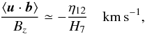 (1)where
H7 = Hρ/100 km
and ηT = 1012 η12
cm2/s. With observations of the left hand side of (1) of about 1 km s-1, one would
find ηT of order 1012 cm2/s. This is in
line with the results from box simulations of mixed-polarity magnetic fields in the solar
surface layer, where values between 1012 cm2/s
and 3.4 × 1012 cm2/s were found (Cameron et al. 2011). In the present paper, numerical simulations of
stratified magnetoconvection and observational results are discussed, and the theory will be
extended to include a vertical stratification of the turbulence intensity. Both the
simulations and the observations lead to very similar results for the desired magnetic eddy
diffusivity for the quiet Sun, exceeding the value given by (1) by a factor of (only) two.
(1)where
H7 = Hρ/100 km
and ηT = 1012 η12
cm2/s. With observations of the left hand side of (1) of about 1 km s-1, one would
find ηT of order 1012 cm2/s. This is in
line with the results from box simulations of mixed-polarity magnetic fields in the solar
surface layer, where values between 1012 cm2/s
and 3.4 × 1012 cm2/s were found (Cameron et al. 2011). In the present paper, numerical simulations of
stratified magnetoconvection and observational results are discussed, and the theory will be
extended to include a vertical stratification of the turbulence intensity. Both the
simulations and the observations lead to very similar results for the desired magnetic eddy
diffusivity for the quiet Sun, exceeding the value given by (1) by a factor of (only) two.
A simple prediction of this theory is that the ratio (1) does not depend on the sign of the mean magnetic field, i.e., it does not vary from cycle to cycle and (for a dipolar field) from hemisphere to hemisphere. As a consequence, the sign of the cross helicity ⟨u·b⟩ should vary from cycle to cycle and between the hemispheres. Zhao et al. (2011) indeed found indications for a variation from hemisphere to hemisphere in magnetograms and dopplergrams recorded by the Solar and Heliospheric Observatory’s Michelson Doppler Imager in 2000, 2004, and 2007.
2. Mean-field electrodynamics
Let U + u and
B + b be the fluctuating
velocity and magnetic field with the average values U and
B. The scalar correlation between the fluctuations of flow
and field, i.e., the cross
helicity ⟨u·b⟩, is a
pseudoscalar. In the same sense, the cross-correlation tensor
⟨uibj⟩
is a pseudotensor. We are here only interested in its symmetric part 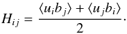 (2)As we have shown, the
tensor Hij can be finite in presence of a mean
magnetic field B and for density-stratified fluids (Rüdiger
et al. 2011). Consider these quantities as small
enough so that expressions linear in the mean magnetic field influence of these quantities
are sufficient. The same may hold for the shear, which influences the (radial) magnetic
field components. It is then straightforward to formulate the relation
(2)As we have shown, the
tensor Hij can be finite in presence of a mean
magnetic field B and for density-stratified fluids (Rüdiger
et al. 2011). Consider these quantities as small
enough so that expressions linear in the mean magnetic field influence of these quantities
are sufficient. The same may hold for the shear, which influences the (radial) magnetic
field components. It is then straightforward to formulate the relation 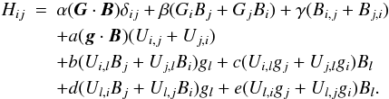 (3)No
other formations are possible linear in the mean field B, the
stratification vector G, and the shear of the divergence-free
mean flow U. For the tensor components, we find
(3)No
other formations are possible linear in the mean field B, the
stratification vector G, and the shear of the divergence-free
mean flow U. For the tensor components, we find  (4)and
 (5)if a box
coordinate system (x,y,z) for the latitudinal, azimuthal, and vertical
direction is introduced. The z-axis is aligned with the stratification
vector, i.e., it represents the radial direction in spherical geometry. The
x and y coordinates denote the horizontal directions.
Without shear, the correlation Hzz measures the
vertical magnetic field and the correlation Hyz
measures the azimuthal field. The correlations are also influenced by the
shear Uy,z. With the shear included, finite
values result for both the correlations (4)
and (5), even when the field has only one
component. For known values of the correlations, the coefficients and the vertical field of
both the azimuthal field and the shear can be computed. We cannot, however,
be sure that all the coefficients a....e
must be nonzero. First test calculations of Hzz
under the presence of horizontal field and shear did not yield finite
values of e (Brandenburg, priv. comm.).
(5)if a box
coordinate system (x,y,z) for the latitudinal, azimuthal, and vertical
direction is introduced. The z-axis is aligned with the stratification
vector, i.e., it represents the radial direction in spherical geometry. The
x and y coordinates denote the horizontal directions.
Without shear, the correlation Hzz measures the
vertical magnetic field and the correlation Hyz
measures the azimuthal field. The correlations are also influenced by the
shear Uy,z. With the shear included, finite
values result for both the correlations (4)
and (5), even when the field has only one
component. For known values of the correlations, the coefficients and the vertical field of
both the azimuthal field and the shear can be computed. We cannot, however,
be sure that all the coefficients a....e
must be nonzero. First test calculations of Hzz
under the presence of horizontal field and shear did not yield finite
values of e (Brandenburg, priv. comm.).
The turbulent flow is assumed anelastic, so that
div ρu = 0. It is convenient to use the
Fourier transformation of the momentum density
m = ρu, i.e.,
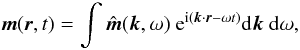 (6)and likewise for the
fluctuation of the magnetic field.
(6)and likewise for the
fluctuation of the magnetic field.
The spectral tensor of the momentum density that accounts for the stratification of the
turbulence to the first-order terms reads 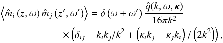 (7)where
k = (z−z′)/2, κ = z + z′,
(7)where
k = (z−z′)/2, κ = z + z′,
 is the Fourier transform of the local spectrum,
 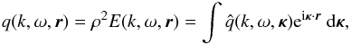 (8)so that
  (9) Derivation of the
cross-correlation yields
(9) Derivation of the
cross-correlation yields 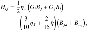 (10)where
G = ∇log ρ is
the gradient of density and
(10)where
G = ∇log ρ is
the gradient of density and 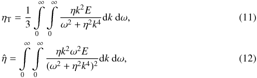 where
η is the molecular magnetic diffusivity. Both quantities remain finite in
the high-conductivity limit.
where
η is the molecular magnetic diffusivity. Both quantities remain finite in
the high-conductivity limit.
From the cross-correlation tensor (10), the
cross helicity
⟨u·b⟩ = ηT(G·B)
is obtained. From Eq. (10) we find the
slightly more complicated expression 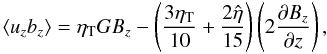 (13)where
G = Gz is the only nonzero
radial component of the density-stratification vector. Note the negativity of
G. An upwards divergence of the mean field would reduce the effect of
density stratification, but for uniform field components, the result is
⟨uzbz⟩ = ⟨u·b⟩.
(13)where
G = Gz is the only nonzero
radial component of the density-stratification vector. Note the negativity of
G. An upwards divergence of the mean field would reduce the effect of
density stratification, but for uniform field components, the result is
⟨uzbz⟩ = ⟨u·b⟩.
A real difference between both correlation expressions is, however, due to a possible
gradient G′ of the turbulence
intensity urms. One easily finds that for vertical fields the
turbulence intensity gradient G′ enters expressions
for the correlations such as 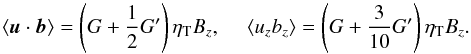 (14)In the bulk of the
convection zone,
(14)In the bulk of the
convection zone,  is positive
while G is negative. Hence,
|⟨uzbz ⟩|>|⟨ u·b⟩|
for positive Bz, which is confirmed by the
presented simulations (see below).
is positive
while G is negative. Hence,
|⟨uzbz ⟩|>|⟨ u·b⟩|
for positive Bz, which is confirmed by the
presented simulations (see below).
By elimination of G′ one finds 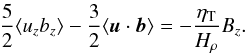 (15)The magnetic eddy
diffusivity can thus be determined if the LHS of (15) is calculated from magnetoconvection simulations when the density scale height
Hρ is known from numerical models of the
solar atmosphere. As only the correlation
⟨uzbz⟩
can directly be observed, one needs a numerical model for the application of the LHS of
(15) to derive the eddy diffusivity at the
solar surface.
(15)The magnetic eddy
diffusivity can thus be determined if the LHS of (15) is calculated from magnetoconvection simulations when the density scale height
Hρ is known from numerical models of the
solar atmosphere. As only the correlation
⟨uzbz⟩
can directly be observed, one needs a numerical model for the application of the LHS of
(15) to derive the eddy diffusivity at the
solar surface.
3. Numerical simulations
We perform simulations for a number of different parameter combinations. These parameters include the strength of the imposed vertical field Bz, the viscosity ν, and the magnetic diffusivity coefficient η.
The numerical simulations are done using the Nirvana code, which uses a conservative finite
difference scheme (Ziegler 2004). We use Cartesian
coordinates. The code solves the equation of motion, ![Mathematical equation: \begin{eqnarray} \frac{\partial (\rho \vec{u})}{\partial t} + \nabla \cdot \left[ \rho \vec{u} \vec{u} + \left(p + \frac{1}{8 \pi}|\vec{B}|^2\right) I - \frac{1}{4 \pi} \vec{B} \vec{B} \right] &=& \nonumber \\ \label{motion} && \!\! \nabla \cdot \tau + \rho \vec{f}_{\rm e}, \end{eqnarray}](/articles/aa/full_html/2012/10/aa19268-12/aa19268-12-eq72.png) (16)the
induction equation,
(16)the
induction equation,  (17)the equation of
mass conservation,
(17)the equation of
mass conservation,  (18)and the equation of energy
conservation,
(18)and the equation of energy
conservation, ![Mathematical equation: \begin{eqnarray} \frac{\partial e}{\partial t} + \nabla \cdot \left[\left(e+p+\frac{1}{8 \pi} |\vec{B}|^2\right)\vec{v} - \frac{1}{4\pi} (\vec{u}\cdot \vec{B}) \vec{B} \right] = \nonumber \\ \nabla \cdot \left[ \vec{u} \tau + \frac{\eta}{4\pi} \vec{B} \times(\nabla \times \vec{B}) - \vec{F}_{\rm cond} \right] +\rho \vec{f}_{\rm e} \cdot \vec{u}. \label{energy} \end{eqnarray}](/articles/aa/full_html/2012/10/aa19268-12/aa19268-12-eq75.png) (19) In
Eqs. (16) and (19), fe
is the (external) gravity force and
(19) In
Eqs. (16) and (19), fe
is the (external) gravity force and  (20)the
viscous stress tensor. The total energy density is the sum of the thermal, kinetic, and
magnetic energy density:
(20)the
viscous stress tensor. The total energy density is the sum of the thermal, kinetic, and
magnetic energy density:  (21) We assume an ideal gas
with a constant mean molecular weight μ = 1. The thermal energy density is
then
(21) We assume an ideal gas
with a constant mean molecular weight μ = 1. The thermal energy density is
then  (22)with
γ = cp/cv = 5/3.
(22)with
γ = cp/cv = 5/3.
The gas is heated from below and kept at a fixed temperature at the top of the simulation box. Periodic boundary conditions apply at the horizontal boundaries. A homogeneous vertical magnetic field is applied. The upper and lower boundaries are impenetrable and stress-free.
The simulation volume is a rectangular box. The stratification is along the z-coordinate, and it is piecewise polytrophic, with the polytrophic index chosen such that the hydrostatic equilibrium state is convectively stable in the lower and unstable in the upper half of the simulation box. In the following, p denotes gas pressure, ρ mass density, T temperature, g gravity, κ thermal conductivity, and cp the specific heat capacity at constant pressure.
The gas is initially in hydrostatic equilibrium, i.e.,
 (23)where
g = const., and the heat flux through the box is
vertical and constant,
(23)where
g = const., and the heat flux through the box is
vertical and constant,  (24)The equation
of state is that for an ideal gas. The heat conductivity is constant in the upper and lower
layer, respectively, but its values differ between the two layers.
(24)The equation
of state is that for an ideal gas. The heat conductivity is constant in the upper and lower
layer, respectively, but its values differ between the two layers.
In the dimensionless units, the size of the simulation box is 8 × 8 × 2 in the x, y, and z directions, respectively. The numerical resolution is 512 × 512 × 128 grid points. The stratification of density, pressure, and temperature is piecewise polytrophic, as described in Ziegler (2002). Similar setups have been used by Cattaneo et al. (1991), Brummell et al. (1996), Brandenburg et al. (1996), Chan (2001) and Ossendrijver et al. (2001). The initial state is in hydrostatic equilibrium but convectively unstable in the upper half of the box. The z coordinate is negative in our setup, with z = 0 at the upper boundary. The stable layer thus extends from z = −2 to z = −1, the unstable layer from z = −1 to z = 0. The density varies by a factor 5 over the depth of the box, i.e., the density scale height is 1.2.
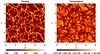 |
Fig. 1 Fluctuations of density and temperature in the upper part of the unstable layer at z = −0.05 for Ra = 107 and B0 = 1. |
Figure 1 shows snapshots of the fluctuations of density and temperature for Ra = 107 in a horizontal plane close to the upper boundary. The density is increased at the boundaries of the convection cells and decreased at the center. The opposite is true for the temperature, which is highest at the center of a convection cell and lowest at the boundaries. Vertical velocity is positive, i.e. upwards, at the center and negative, i.e. downwards, at the boundaries. The magnetic field is strongly concentrated in a few small patches which coincide with cell corners, where the gas horizontal flow converges and the vertical flow is downwards.
The initial magnetic field is vertical and homogeneous. We run the simulations until a
quasistationary state evolves. Our control parameters are the heat conduction coefficient
κ and the Prandtl number Pr =
ν/κ. Convection sets in if the
Rayleigh number 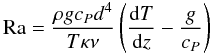 (25)with
the density ρ, the specific heat capacity cP,
the gravity force g, and the length scale d, exceeds a
critical value. The length scale is defined by the depth of the convectively unstable layer,
i.e., d = 1. After (1), the
correlations and the mean magnetic field always have opposite signs. This has also been
confirmed numerically. For positive values of the mean magnetic field
Bz, the cross helicity is negative in the
unstably stratified layer. If the field polarity is reversed and everything else is left
unchanged the cross-correlation becomes positive with the same amplitude.
(25)with
the density ρ, the specific heat capacity cP,
the gravity force g, and the length scale d, exceeds a
critical value. The length scale is defined by the depth of the convectively unstable layer,
i.e., d = 1. After (1), the
correlations and the mean magnetic field always have opposite signs. This has also been
confirmed numerically. For positive values of the mean magnetic field
Bz, the cross helicity is negative in the
unstably stratified layer. If the field polarity is reversed and everything else is left
unchanged the cross-correlation becomes positive with the same amplitude.
The velocity field, which is measured in units of cac/100, shows the asymmetry between upwards and downwards motion as characteristic of convection in stratified media. The downwards motion is concentrated at the boundaries of the convection cells and particularly at the corners. The upwards motion fills the interior of the convection cells (see Fig. 2). As it covers a much larger area, the gas motion is considerably slower than in the concentrated downdrafts. The magnetic field shows a similar pattern. The vertical field is concentrated in the areas with downwards motion and weak in the areas with upwards motion. This is the result of field advection, as the total vertical magnetic flux is conserved.
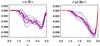 |
Fig. 3 Numerical values for the cross helicity ⟨u·b⟩ (left) and the coefficient ⟨uzbz⟩ (right) for weak magnetic field Bz = 10-3. The blue lines denote individual snapshots, and the red lines average over the snapshots shown. |
Figures 3 and 4
hold for Ra = 107 and for weak and strong magnetic fields. The value of both the
Prandtl number and the magnetic Prandtl number is 0.1. The left diagram shows the horizontal
average of the cross helicity as a function of the depth, and the right diagram shows the
same for the correlation of the vertical components,
⟨uzbz⟩.
There is a difference between the two quantities, with the vertical component actually being
twice the cross helicity. Equation (15) can
thus be written as 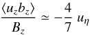 (26)with
 (27)The correlations do
not vanish abruptly at the bottom of the unstable layer because of overshoot, which affects
the upper half of the stable layer. The correlations there are positive and much smaller
than in the unstable layer.
(27)The correlations do
not vanish abruptly at the bottom of the unstable layer because of overshoot, which affects
the upper half of the stable layer. The correlations there are positive and much smaller
than in the unstable layer.
The results in Fig. 3 are given in arbitrary units
defined by the code. Velocities are given in units of
cac/100 with the isothermal speed of sound
cac. With an approximate value
of cac ≃ 6.6 km s-1 at the optical depth
τ = 1 of the Sun, the simulations lead to the cross-correlation velocity
⟨uzbz⟩/Bz ≃ −9
in units of 0.066 km s-1 (Fig. 3, right),
i.e., after (26)  (28)This value depends only
slightly on the magnetic field amplitude for weak fields. For the much stronger magnetic
field, Fig. 4 (right) yields the slightly smaller value
of 0.81 km s-1.
(28)This value depends only
slightly on the magnetic field amplitude for weak fields. For the much stronger magnetic
field, Fig. 4 (right) yields the slightly smaller value
of 0.81 km s-1.
A characteristic velocity results as the cross-correlation velocity  (29)Using the
maximal values in Fig. 3 (left), we
find Uc ≃ 6 in units of
cac/100. Hence, the simulations lead to the
cross-correlation velocity Uc ≃ 0.4 km s-1. For the
Bz = 1 case (Fig. 4, left), we find Uc ≃ 3 in units of
cac/100 or 0.2 km s-1,
respectively.
(29)Using the
maximal values in Fig. 3 (left), we
find Uc ≃ 6 in units of
cac/100. Hence, the simulations lead to the
cross-correlation velocity Uc ≃ 0.4 km s-1. For the
Bz = 1 case (Fig. 4, left), we find Uc ≃ 3 in units of
cac/100 or 0.2 km s-1,
respectively.
It also makes sense to normalize the cross-correlation in the form  (30)which is the ratio of the
cross-correlation velocity (29) and the rms
velocity of the turbulence. Its numerical value does not depend on the internal units of the
code, so that cη is a general and basic result
of the simulations. Close to the surface, the maximal numerical value
is cη ≃ 0.6
for Bz = 10-3
and cη ≃ 0.3
for Bz = 1. Test calculations for various
magnetic fields over many orders of magnitudes show this value as almost uninfluenced by the
magnetic-field suppression. Resulting from the overshoot phenomenon at the bottom of the
unstable layer, small negative values always appear there. The correlation coefficient
(30)which is the ratio of the
cross-correlation velocity (29) and the rms
velocity of the turbulence. Its numerical value does not depend on the internal units of the
code, so that cη is a general and basic result
of the simulations. Close to the surface, the maximal numerical value
is cη ≃ 0.6
for Bz = 10-3
and cη ≃ 0.3
for Bz = 1. Test calculations for various
magnetic fields over many orders of magnitudes show this value as almost uninfluenced by the
magnetic-field suppression. Resulting from the overshoot phenomenon at the bottom of the
unstable layer, small negative values always appear there. The correlation coefficient
 (31)for the cross helicity is
much smaller than (30) as always
(31)for the cross helicity is
much smaller than (30) as always
 (32)similar to the result of
Ossendrijver et al. (2001). The relation (31) proves to be true for all amplitudes of the
mean magnetic field between 10-5 and 0.1. One finds for all calculations a
characteristic correlation coefficient c ≃ 0.1. The
Bz = 1 case shows the beginning of the
suppression of the fluctuations by the mean magnetic field, which occurs at large values of
Bz, resulting in a smaller value of 25 for
(32)similar to the result of
Ossendrijver et al. (2001). The relation (31) proves to be true for all amplitudes of the
mean magnetic field between 10-5 and 0.1. One finds for all calculations a
characteristic correlation coefficient c ≃ 0.1. The
Bz = 1 case shows the beginning of the
suppression of the fluctuations by the mean magnetic field, which occurs at large values of
Bz, resulting in a smaller value of 25 for
 .
.
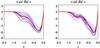 |
Fig. 5 The same as in the right part of Fig. 4 but with reduced numerical resolution of 128 × 128 × 128 (left) and 256 × 256 × 128 (right). |
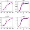 |
Fig. 6 Numerical values for urms (left) and brms (right) for weak magnetic field, Bz = 10-3 (top) and strong magnetic field, Bz = 1 (bottom). Only the magnetic fluctuations depend on the background field amplitude. |
During the simulations, there are significant temporal fluctuations. The convective instability initially grows exponentially until its saturation, when the system settles in a statistically steady state, but the cross helicity still shows some variations. We therefore average over a certain number of snapshots, typically ten. To test how much the results depend on the numerical resolution, we rerun the Bz = 1 case at the lower resolutions of 256 × 256 × 128 and 1283. Figure 5 shows ⟨uzbz⟩ from those runs. There is a weak dependence on resolution, with higher resolution leading to larger values.
Figure 6 contains all the information about the
kinetic and magnetic energies of the magnetoconvection. The rms value of the velocity is
hardly influenced by the large-scale magnetic field. In physical units, we find an averaged
value of
urms ≃ 0.1cac ≃ 0.66 km s-1.
In contrast, the magnetic energy strongly depends on the applied magnetic field. In
dimensionless units, it is
brms/urms ≃ 0.6Bz
in both cases, which leads to  (33)in
physical units. At the top of the convection zone, we find very small contributions of the
magnetic energy for Bz = 1 Gauss, while for
1000 Gauss there is almost equipartition.
(33)in
physical units. At the top of the convection zone, we find very small contributions of the
magnetic energy for Bz = 1 Gauss, while for
1000 Gauss there is almost equipartition.
Results from the analysis of the SST and Hinode data.
4. Observations
It is difficult to empirically determine the cross helicity ⟨u·b⟩ at the solar surface because it is hard to retrieve the horizontal flows and magnetic field components from observations. We have, however, the possibility to use the relation ⟨u·b⟩ ≈ 0.5⟨uzbz⟩, known from the above numerical simulations. The vertical flow speed and magnetic field component can be determined with much better accuracy. Then using Eq. (26), we can determine the cross-helicity velocity from the observations.
For this purpose, we have analysed two datasets containing observations of the quiet Sun at
disk center, where the line-of-sight coincides with the local vertical. Data from the Crisp
Imaging Solar Polarimeter (CRISP) instrument on the Swedish 1-m Solar Telescope (SST) cover
the 6302.5 Å Fe i spectral line with 12 equidistant wavelength positions at 48 mÅ
steps and a continuum point. They have a pixel scale of
 and a total field-of-view
of about 60′′ × 60′′. The second dataset is from the
spectropolarimeter on the Solar Optical Telescope (SOT) of Hinode. It covers both the 6301.5
and 6302.5 Å Fe i lines, has a pixel scale of
and a total field-of-view
of about 60′′ × 60′′. The second dataset is from the
spectropolarimeter on the Solar Optical Telescope (SOT) of Hinode. It covers both the 6301.5
and 6302.5 Å Fe i lines, has a pixel scale of
 , and a total (scanned) field
of view of 164′′ × 328′′.
, and a total (scanned) field
of view of 164′′ × 328′′.
The line-of-sight velocity and magnetic field data for the Hinode observations were taken from the level two data products available online1. Magnetic field strengths have been converted to fluxes by taking the filling factor into account. The SST data were inverted using the lilia inversion code (Socas-Navarro 2001). Velocities were calibrated using the convective blueshift determined by de La Cruz Rodríguez et al. (2011). More details on these two datasets can be found in Schnerr & Spruit (2011).
We show the results for these datasets in Table 1. The cross-helicity velocity (uη) as determined from the SST data is somewhat higher than that from the Hinode data. This is at least partly due to the lower resolution of Hinode as compared to the SST. If we rebin the SST data to a lower resolution, the cross-helicity velocity decreases (see Table 1) because the strongest fields and flows are smoothed out.
The coefficient  from the Hinode and
SST data is 521.3 and 163.5 respectively, which is larger than the value of 50 found in the
simulations. This indicates that the effective magnetic Reynolds number in the simulations
is smaller than in the solar convection zone.
from the Hinode and
SST data is 521.3 and 163.5 respectively, which is larger than the value of 50 found in the
simulations. This indicates that the effective magnetic Reynolds number in the simulations
is smaller than in the solar convection zone.
5. Conclusions
We have shown that nonrotating turbulence at the top of the solar convection zone under the influence of a vertical magnetic field forms a finite cross helicity. The only condition is the existence of a vertical stratification of density and/or turbulence intensity. While the effect would not appear within the Boussinesq approximation, it exists in the high-conductivity limit, i.e., for sufficiently large magnetic Reynolds numbers.
In our understanding, the cross helicity is anticorrelated to the mean radial magnetic
field, i.e.,  (34)For an oscillating
dipolar background field, the sign of the cross helicity differs for both hemispheres and
also from cycle to cycle.
(34)For an oscillating
dipolar background field, the sign of the cross helicity differs for both hemispheres and
also from cycle to cycle.
The theory can also be used to measure the magnetic diffusivity if the cross helicity is known by observations. In order to find the cross helicity, one has only to correlate observed flow fluctuations with observed magnetic fluctuations.
The anticorrelation (34) for density-stratified turbulence has been established by Rüdiger et al. (2011) for a model of numerically-driven turbulence. In the present paper, buoyancy-driven magnetoconvection has been simulated in a box with the Nirvana code. We find that such a turbulence also fulfills the relation (34). The correlation coefficient (30) takes the value of 0.6 for the weak magnetic field Bz = 10-3 and 0.3 for the stronger field Bz = 1. The ratio (32) of the magnetic fluctuations to the applied magnetic field is always of the order five.
We have also shown that for density-stratified turbulence the identity ⟨u·b⟩ = ⟨uzbz⟩ holds. So far, solar observations can only measure the correlation ⟨uzbz⟩. The numerical simulations,
however, always lead to the result ⟨uzbz⟩ ≃ 2⟨u·b⟩, so that the observed value of ⟨uzbz⟩ would overestimate the actual cross helicity by a factor of two. The reason is the vertical stratification of the turbulence intensity, which at the top of the convection zone is antiparallel to the density stratification. Hence, both the correlations ⟨uzbz⟩ and ⟨u·b⟩ are reduced but not by the same amount.
With ⟨uzbz⟩ ≃ 2⟨u·b⟩, the value of uη can be computed by using Eq. (26). The numerical simulations lead to uη ≃ 1 km s-1 and uη ≃ 0.8 km s-1 respectively for the two cases studied. This result is well confirmed by the observations that lead to values between 0.7 km s-1 (Hinode) and 1.3 km s-1 (SST). To estimate the value of the eddy diffusivity at the solar surface, we shall assume a density scale height of 100 km and find values close to ηT ≃ 1012 cm2/s for the eddy diffusivity at the surface of the quiet Sun.
Acknowledgments
We gratefully acknowledge Axel Brandenburg (Stockholm) for motivating discussions and numerical support.
References
- Brandenburg, A., Jennings, R. L., Nordlund, Å., et al. 1996, JFM, 306, 325 [Google Scholar]
- Brummell, N. H., Hurlburt, N. E., & Toomre, J. 1996, ApJ, 473, 494 [NASA ADS] [CrossRef] [Google Scholar]
- Cameron, R., Vögler, A., & Schüssler, M. 2011, A&A, 533, A86 [NASA ADS] [CrossRef] [EDP Sciences] [Google Scholar]
- Cattaneo, F., Brummell, N. H., Toomre, J., Malagoli, A., & Hurlburt, N. E. 1991, ApJ, 370, 282 [NASA ADS] [CrossRef] [Google Scholar]
- Chan, K. L. 2001, ApJ, 548, 1102 [NASA ADS] [CrossRef] [Google Scholar]
- de La Cruz Rodríguez, J., Kiselman, D., & Carlsson, M. 2011, A&A, 528, A113 [NASA ADS] [CrossRef] [EDP Sciences] [Google Scholar]
- Ossendrijver, M., Stix, M., & Brandenburg, A. 2001, A&A, 376, 713 [NASA ADS] [CrossRef] [EDP Sciences] [Google Scholar]
- Rüdiger, G., Kitchatinov, L. L., & Brandenburg, A. 2011, Sol. Phys., 269, 3 [NASA ADS] [CrossRef] [MathSciNet] [Google Scholar]
- Schnerr, R. S., & Spruit, H. C. 2011, A&A, 532, A136 [NASA ADS] [CrossRef] [EDP Sciences] [Google Scholar]
- Schrijver, C. J., & Martin, S. F. 1990, Sol. Phys., 129, 95 [NASA ADS] [CrossRef] [Google Scholar]
- Socas-Navarro, H. 2001, in Advanced Solar Polarimetry – Theory, Observation, and Instrumentation, ed. Sigwarth, ASPCS, 236, 487 [Google Scholar]
- Stix, M. 1989, The Sun: An Introduction (Berlin, Heidelberg, New York: Springer) [Google Scholar]
- Zhao, M. Y., Wang, X. W., & Zhang, H. Q. 2011, Sol. Phys., 270, 23 [NASA ADS] [CrossRef] [Google Scholar]
- Ziegler, U. 2002, A&A, 386, 331 [NASA ADS] [CrossRef] [EDP Sciences] [Google Scholar]
- Ziegler, U. 2004, J. Comput. Phys., 196, 393 [NASA ADS] [CrossRef] [Google Scholar]
All Tables
All Figures
|
Fig. 1 Fluctuations of density and temperature in the upper part of the unstable layer at z = −0.05 for Ra = 107 and B0 = 1. |
| In the text | |
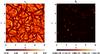 |
Fig. 2 The same as in Fig. 1 but for the fluctuations of the vertical flow and the vertical field. |
| In the text | |
|
Fig. 3 Numerical values for the cross helicity ⟨u·b⟩ (left) and the coefficient ⟨uzbz⟩ (right) for weak magnetic field Bz = 10-3. The blue lines denote individual snapshots, and the red lines average over the snapshots shown. |
| In the text | |
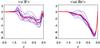 |
Fig. 4 The same as in Fig. 3 but for B0 = 1. |
| In the text | |
|
Fig. 5 The same as in the right part of Fig. 4 but with reduced numerical resolution of 128 × 128 × 128 (left) and 256 × 256 × 128 (right). |
| In the text | |
|
Fig. 6 Numerical values for urms (left) and brms (right) for weak magnetic field, Bz = 10-3 (top) and strong magnetic field, Bz = 1 (bottom). Only the magnetic fluctuations depend on the background field amplitude. |
| In the text | |
Current usage metrics show cumulative count of Article Views (full-text article views including HTML views, PDF and ePub downloads, according to the available data) and Abstracts Views on Vision4Press platform.
Data correspond to usage on the plateform after 2015. The current usage metrics is available 48-96 hours after online publication and is updated daily on week days.
Initial download of the metrics may take a while.