© ESO, 2012

1. Introduction

Gaia (e.g., Perryman et al. 2001; Lindegren et al. 2008) is the upcoming astrometry mission of the European Space Agency (ESA), following up on the success of the Hipparcos mission (ESA 1997a; Perryman et al. 1997; Perryman 2009). Gaia’s science objective is to unravel the kinematical, dynamical, and chemical structure and evolution of our galaxy, the Milky Way (e.g., Gómez et al. 2010). In addition, Gaia’s data will revolutionise many other areas of (astro)physics, e.g., stellar structure and evolution, stellar variability, double and multiple stars, solar-system bodies, fundamental physics, and exo-planets (e.g., Pourbaix 2008; Tanga et al. 2008; Mignard & Klioner 2010; Eyer et al. 2011; Sozzetti 2011; Mouret 2011). During its five-year lifetime, Gaia will survey the full sky and repeatedly observe the brightest 1000 million objects, down to 20th magnitude (e.g., de Bruijne et al. 2010). Gaia’s science data comprises absolute astrometry, broad-band photometry, and low-resolution spectro-photometry. Medium-resolution spectroscopic data will be obtained for the brightest 150 million sources, down to 17th magnitude. The final Gaia catalogue, due in ~2021, will contain astrometry (positions, parallaxes, and proper motions) with standard errors less than 10 micro-arcsecond (μas, μas yr^-1 for proper motions) for stars brighter than 12 mag, 25 μas for stars at 15th magnitude, and 300 μas at magnitude 20 (de Bruijne 2012). Milli-magnitude-precision photometry (Jordi et al. 2010) allows to get a handle on effective temperature, surface gravity, metallicity, and reddening of all stars (Bailer-Jones 2010). The spectroscopic data allows the determination of radial velocities with errors of 1 km s^-1 at the bright end and 15 km s^-1 at magnitude 17 (Wilkinson et al. 2005; Katz et al. 2011) as well as astrophysical diagnostics such as effective temperature and metallicity for the brightest few million objects (Kordopatis et al. 2011). Clearly, these performances will only be reached with a total of five years of collected data and only after careful calibration.

Intermediate releases of the data – obviously with lower quality and/or reduced contents compared to the final catalogue – are planned, the first one around two years after launch, which is currently foreseen for the second half of 2013. The Hundred-Thousand-Proper-Motion (HTPM) project (Mignard 2009), conceived and led by François Mignard at the Observatoire de la Côte d’Azur, is part of the first intermediate release. Its goal is to determine the absolute proper motions of the ~113   500 brightest stars in the sky using Hipparcos astrometry for the first epoch and early Gaia astrometry for the second. Clearly, the HTPM catalogue will have a limited lifetime since it will be superseded by the final Gaia catalogue in ~2021. Nevertheless, the HTPM is a scientifically interesting as well as unique catalogue: the ~23-year temporal baseline, with a mean Hipparcos epoch of 1991.25 and a mean Gaia epoch around 2014.5, allows a significant improvement of the Hipparcos proper motions, which have typical precisions at the level of 1 milli-arcsec yr^-1 (mas yr^-1): the expected HTPM proper-motion standard errors¹ are 40−190 μas yr^-1 for the proper motion in right ascension μ_α ^∗  and 30−150 μas yr^-1 for the proper motion in declination μ_δ, primarily depending on magnitude (we use the common Hipparcos notation α ^∗  = α   cosδ; ESA 1997a, Sect. 1.2.5). A clear advantage of combining astrometric data from the Hipparcos and Gaia missions is that the associated proper motions will be, by construction and IAU resolution, in the system of the International Celestial Reference System (ICRS), i.e., the proper motions will be absolute rather than relative. In this light, it is important to realise that massive, modern-day proper-motion catalogues, such as UCAC-3 (Zacharias et al. 2010), often contain relative proper motions only and that they can suffer from substantial, regional, systematic distortions in their proper-motion systems, up to levels of 10 mas yr^-1 or more (e.g., Röser et al. 2008, 2010; Liu et al. 2011).

It is a well-known geometrical feature, for instance already described by Seeliger in 1900, that for fast-moving, nearby stars, it is essential to know the radial velocity for a precise measurement and determination of proper motion. In fact, this so-called secular or perspective acceleration on the sky was taken into account in the determination of the Hipparcos proper motions for 21 stars (ESA 1997a, Sect. 1.2.8) and the same will be done for Gaia, albeit for a larger sample of nearby stars. Clearly, the inverse relationship also holds: with a precise proper motion available, a so-called astrometric radial velocity can be determined, independent of the spectroscopically measured quantity (see Lindegren & Dravins 2003, for a precise definition and meaning of [astrometric] radial velocity). With this method, Dravins et al. (1999) determined² the astrometric radial velocities for 17 stars, from Hipparcos proper motions combined with Astrographic Catalogue positions at earlier epochs. Although Dravins et al. (1999) reached relatively modest astrometric-radial-velocity precisions, typically a few tens of km s^-1, their results are interesting since they provide direct and independent constraints on various physical phenomena affecting spectroscopic radial velocities, for instance gravitational redshifts, stellar rotation, convection, and pulsation. In our study, however, we approach (astrometric) radial velocities from the other direction since our interest is to determine accurate HTPM proper motions which are not biased by unmodelled perspective effects. In other words: we aim to establish for which stars in the forthcoming HTPM catalogue the currently available (spectroscopic) radial velocity and associated standard error are sufficient to guarantee, with a certain confidence level, a negligible perspective-acceleration-induced error in the HTPM proper motion. For stars without a literature value of the radial velocity, we establish whether – and, if yes, with what standard error – a radial velocity needs to be acquired prior to the construction of the HTPM catalogue. Section 2 describes the available astrometric and spectroscopic data. The propagation model of star positions is outlined in Sect. 3. We investigate the influence of the radial velocity on HTPM proper motions in Sect. 4 and develop two evaluation criteria in Sect. 5. We employ these in Sect. 6. We discuss our results in Sect. 7 and give our final conclusions in Sect. 8.

2. The XHIP catalogue

As source for the Hipparcos astrometry and literature radial velocities, we used the eXtended Hipparcos compilation catalogue (CDS catalogue V/137), also known as XHIP (Anderson & Francis 2012). This catalogue complements the 117 955 entries with astrometry in the Hipparcos catalogue with a set of 116 096 spectral classifications, 46 392 radial velocities, and 18 549 iron abundances from various literature sources.

2.1. Astrometry

The starting point for the XHIP compilation was the new reduction of the Hipparcos data (van Leeuwen 2007, 2008, CDS catalogue I/311), also known as HIP-2. Realising that stars with multiple components were solved individually, rather than as systems, by van Leeuwen for the sake of expediency, Anderson & Francis reverted to the original HIP-1 astrometry (ESA 1997a,b, CDS catalogue I/239) in those cases where multiplicity is indicated and where the formal parallax standard error in HIP-2 exceeds that in HIP-1. This applies to 1922 entries. In addition, Anderson & Francis included the Tycho-2 catalogue (Høg et al. 2000a,b, CDS catalogue I/259) in their XHIP proper-motion data. In the absence of Tycho-2 proper motions, HIP-2 proper motions were forcibly used. When multiplicity is indicated, Hipparcos proper motions were replaced by Tycho-2 values in those cases where the latter are more precise. When multiplicity is not indicated, Tycho-2 proper motions replaced Hipparcos values if the associated standard errors exceed the Tycho-2 standard errors by a factor three or more. In all other cases, a mean HIP-2 – Tycho-2 proper motion was constructed and used, weighted by the inverse squared standard errors; this applies to 92 269 entries.

2.2. Radial velocities

The XHIP catalogue contains radial velocities for 46 392 of the 117 955 entries, carefully compiled by Anderson & Francis from 47 literature sources. The vast majority of measurements have formal measurement precisions, i.e., radial-velocity standard errors (1753 measurements lack standard errors; see Sect. 6.2). In addition, all radial velocities have a quality flag:

• An “A” rating (35 932 entries) indicates that thestandard errors are generally reliable.

• A “B” rating (4239 entries) indicates potential, small, uncorrected, systematic errors.

• A “C” rating (3465 entries) indicates larger systematic errors, while not excluding suitability for population analyses.

• A “D” rating (2756 entries) indicates serious problems, meaning that these stars may not be suitable for statistical analyses. A “D” rating is assigned whenever:

  • 1.

    the radial-velocity standard error is not available;

  • 2.

    the star is an un(re)solved binary;

  • 3.

    the star is a Wolf-Rayet star or a white dwarf that is not a component of a resolved binary; or

  • 4.

    different measurements yield inconsistent results.

The majority of stars in the XHIP catalogue (71 563 entries to be precise) have no measured radial velocity. All we can reasonably assume for these stars is that their radial-velocity distribution is statistically identical to the radial-velocity distribution of the entries with known radial velocities. Figure 1 shows this distribution. It is fairly well represented by a normal distribution with a mean μ = −2.21 km s^-1 and standard deviation σ = 22.44 km s^-1 (the median is −2.00 km s^-1). The observed distribution has low-amplitude, broad wings as well as a small number of real “outliers”, with heliocentric radial velocities up to plus-or-minus several hundred km s^-1. A small fraction of these stars are early-type runaway³ stars (Hoogerwerf et al. 2001) but the majority represent nearby stars in the (non-rotating) halo of our galaxy. The bulk of the stars, those in the main peak, are (thin-)disc stars, co-rotating with the Sun around the galactic centre. In theory, the main peak can be understood, and also be modelled in detail and hence be used to statistically predict the radial velocities for objects without literature values, as a combination of the reflex of the solar motion with respect to the local standard of rest (Delhaye 1965; Schönrich et al. 2010), the effect of differential galactic rotation (Oort 1927), and the random motion of stars (Schwarzschild 1907). In practice, however, such a modelling effort would be massive, touching on a wide variety of (sometimes poorly understood) issues such as the asymmetric drift, the tilt and vertex deviation of the velocity ellipsoid, mixing and heating of stars as function of age, the height of the sun above the galactic plane (Joshi 2007), the dynamical coupling of the local kinematics to the galactic bar and spiral arms (Antoja et al. 2011), large-scale deviations of the local velocity field caused by the Gould Belt (Elias et al. 2006), migration of stars in the disc (Schönrich & Binney 2009), etc. To model these effects, and hence be able to predict a more refined radial velocity for any star as function of its galactic coordinates, distance, and age, is clearly beyond the scope of this paper. We will come back to this issue in Sect. 6.2.

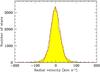Fig. 1 Distribution of all 46 392 radial velocities contained in the XHIP catalogue. The smooth, red curve fits the histogram with a Gaussian normal distribution. The best-fit mean and standard deviation are μ = −2.21 km s-1 and σ = 22.44 km s-1, respectively.

3. Propagation model

3.1. The full model

Let us denote the celestial position of a star at time t₀ (in years) in equatorial coordinates in radians by (α₀,δ₀), its distance in parsec by r = 1000   ϖ^-1, with the parallax ϖ in mas, and its proper-motion components in equatorial coordinates in mas yr^-1 by (μ_α,μ_δ). The three-dimensional position of a star in Cartesian equatorial coordinates at time t₀ is then given by: $\begin{array}{ccc}{\mathit{x}}_{\mathrm{0}}& \mathrm{=}& \mathit{r}\hspace{0.17em}\cos {\mathit{\alpha }}_{\mathrm{0}}\cos {\mathit{\delta }}_{\mathrm{0}}\mathrm{;}\\ {\mathit{y}}_{\mathrm{0}}& \mathrm{=}& \mathit{r}\hspace{0.17em}\sin {\mathit{\alpha }}_{\mathrm{0}}\cos {\mathit{\delta }}_{\mathrm{0}}\mathrm{;}\\ {\mathit{z}}_{\mathrm{0}}& \mathrm{=}& \mathit{r}\hspace{0.17em}\sin {\mathit{\delta }}_{\mathrm{0}}\mathit{.}\end{array}$(1)With v_r the star’s radial velocity in km s^-1, it is customary to define the “radial proper motion” as μ_r = v_r   r^-1. The linear velocity in pc yr^-1 is then given by: $\begin{array}{ccc}{\mathit{v}}_{\mathit{\alpha }}& \mathrm{=}& {\mathit{\mu }}_{\mathit{\alpha }}\hspace{0.17em}\mathit{B}{\mathit{A}}_{\mathrm{V}}{\mathit{\varpi }}^{-1}\mathrm{;}\\ {\mathit{v}}_{\mathit{\delta }}& \mathrm{=}& {\mathit{\mu }}_{\mathit{\delta }}\hspace{0.17em}\mathit{B}{\mathit{A}}_{\mathrm{V}}{\mathit{\varpi }}^{-1}\mathrm{;}\\ {\mathit{v}}_{\mathit{r}}& \mathrm{=}& {\mathit{\mu }}_{\mathit{r}}\hspace{0.17em}\mathit{B,}\end{array}$(2)where A_V = 4.740,470,446 km yr s^-1 is the astronomical unit and the factor $\mathit{B}\mathrm{=}{\mathit{A}}_{\mathrm{p}}\mathrm{\times }{\mathit{A}}_{\mathit{z}}^{-1}\mathrm{=}\mathrm{1.022}\mathit{,}\mathrm{712}\mathit{,}\mathrm{169}\mathrm{\times }{\mathrm{10}}^{-6}$ pc s km^-1 yr^-1 changes km s^-1 to pc yr^-1 (ESA 1997a, Table 1.2.2) so that B × A_V = 4.848,136,811 × 10^-6 pc AU^-1. Transforming these equations into Cartesian coordinates leads to: $\begin{array}{ccc}{\mathit{v}}_{\mathit{x}}& \mathrm{=}& \mathrm{-}{\mathit{v}}_{\mathit{\alpha }}\sin {\mathit{\alpha }}_{\mathrm{0}}\mathrm{-}{\mathit{v}}_{\mathit{\delta }}\cos {\mathit{\alpha }}_{\mathrm{0}}\sin {\mathit{\delta }}_{\mathrm{0}}\mathrm{+}{\mathit{v}}_{\mathit{r}}\cos {\mathit{\alpha }}_{\mathrm{0}}\cos {\mathit{\delta }}_{\mathrm{0}}\mathrm{;}\\ {\mathit{v}}_{\mathit{y}}& \mathrm{=}& {\mathit{v}}_{\mathit{\alpha }}\cos {\mathit{\alpha }}_{\mathrm{0}}\mathrm{-}{\mathit{v}}_{\mathit{\delta }}\sin {\mathit{\alpha }}_{\mathrm{0}}\sin {\mathit{\delta }}_{\mathrm{0}}\mathrm{+}{\mathit{v}}_{\mathit{r}}\sin {\mathit{\alpha }}_{\mathrm{0}}\cos {\mathit{\delta }}_{\mathrm{0}}\mathrm{;}\\ {\mathit{v}}_{\mathit{z}}& \mathrm{=}& {\mathit{v}}_{\mathit{\delta }}\cos {\mathit{\delta }}_{\mathrm{0}}\mathrm{+}{\mathit{v}}_{\mathit{r}}\sin {\mathit{\delta }}_{\mathrm{0}}\mathit{.}\end{array}$(3)Since the motion of stars, or the barycentre of multiple systems, is to near-perfect approximation rectilinear over time scales of a few decades, the position of a star at time t₁, after a time t = t₁ − t₀, now simply follows by applying the propagation model: $\begin{array}{ccc}\mathit{x}\mathrm{\left(}\mathit{t}\mathrm{\right)}& \mathrm{=}& {\mathit{x}}_{\mathrm{0}}\mathrm{+}{\mathit{v}}_{\mathit{x}}\hspace{0.17em}\mathit{t}\mathrm{;}\\ \mathit{y}\mathrm{\left(}\mathit{t}\mathrm{\right)}& \mathrm{=}& {\mathit{y}}_{\mathrm{0}}\mathrm{+}{\mathit{v}}_{\mathit{y}}\hspace{0.17em}\mathit{t}\mathrm{;}\\ \mathit{z}\mathrm{\left(}\mathit{t}\mathrm{\right)}& \mathrm{=}& {\mathit{z}}_{\mathrm{0}}\mathrm{+}{\mathit{v}}_{\mathit{z}}\hspace{0.17em}\mathit{t}\mathit{.}\end{array}$(4)Transforming this back into equatorial coordinates returns the celestial position (α(t),δ(t)) of the star at time t: $\begin{array}{ccc}\mathit{\alpha }\mathrm{\left(}\mathit{t}\mathrm{\right)}& \mathrm{=}& \arctan \left[\frac{\mathit{y}\mathrm{\left(}\mathit{t}\mathrm{\right)}}{\mathit{x}\mathrm{\left(}\mathit{t}\mathrm{\right)}}\right]\mathrm{;}\\ \mathit{\delta }\mathrm{\left(}\mathit{t}\mathrm{\right)}& \mathrm{=}& \arctan \left[\frac{\mathit{z}\mathrm{\left(}\mathit{t}\mathrm{\right)}}{\sqrt{\mathit{x}\mathrm{(}\mathit{t}{\mathrm{)}}^{\mathrm{2}}\mathrm{+}\mathit{y}\mathrm{(}\mathit{t}{\mathrm{)}}^{\mathrm{2}}}}\right]\mathrm{·}\end{array}$(5)So, in summary, it is straightforward to compute the future position of a star on the sky once the initial celestial coordinates, the proper motion, parallax, radial velocity, and time interval are given. This, however, is what nature and Gaia will do for us: the initial celestial coordinates correspond to the Hipparcos epoch (1991.25) and the final coordinates (α(t),δ(t)), with t ≈ 23 yr, will come from the first Gaia astrometry. The HTPM project will determine the proper-motion components (μ_α,μ_δ) from known initial and final celestial coordinates for given time interval, parallax, and radial velocity. Unfortunately, it is not possible to express the proper-motion components in a closed (analytical) form as function of (α₀,δ₀), (α(t),δ(t)), ϖ, v_r, and t since the underlying set of equations is coupled. The derivation of the proper-motion components hence requires a numerical solution. We implemented this solution using Newton-Raphson iteration and refer to this solution as the “full model”. This model, however, is relatively slow for practical implementation. We hence decided to also implement a “truncated model” with analytical terms up to and including t³ (Sect. 3.2), which is about ten times faster and sufficiently precise for our application (Sect. 3.3).

3.2. The truncated model

Mignard (2009) shows that the full model (Sect. 3.1) can be truncated up to and including third-order terms in time t without significant loss in accuracy (Sect. 3.3). Equations (6) and (7) below show the forward propagation for right ascension and declination, respectively. By forward propagation, we mean computing the positional displacements Δα and Δδ of a star for given proper motion, parallax, radial velocity, and time interval t = t₁ − t₀: $\begin{array}{ccc}\mathrm{\Delta }{\mathit{\alpha }}^{\mathrm{\ast }}& \mathrm{=}& \mathrm{\Delta }\mathit{\alpha }\cos {\mathit{\delta }}_{\mathrm{0}}\mathrm{=}\mathrm{\left(}\mathit{\alpha }\mathrm{\right(}\mathit{t}\mathrm{)}\mathrm{-}{\mathit{\alpha }}_{\mathrm{0}}\mathrm{)}\cos {\mathit{\delta }}_{\mathrm{0}}\mathrm{=}\mathrm{+}\left[{\mathit{\mu }}_{\mathit{\alpha }}\right]{\mathit{t}}^{\mathrm{1}}\\ & \mathrm{-}& \left[{\mathit{\mu }}_{\mathit{r}}{\mathit{\mu }}_{\mathit{\alpha }}\mathrm{-}\tan {\mathit{\delta }}_{\mathrm{0}}{\mathit{\mu }}_{\mathit{\alpha }}{\mathit{\mu }}_{\mathit{\delta }}\right]{\mathit{t}}^{\mathrm{2}}\\ & \mathrm{+}& \left[{\mathit{\mu }}_{\mathit{r}}^{\mathrm{2}}{\mathit{\mu }}_{\mathit{\alpha }}\mathrm{-}\mathrm{2}\tan {\mathit{\delta }}_{\mathrm{0}}{\mathit{\mu }}_{\mathit{r}}{\mathit{\mu }}_{\mathit{\alpha }}{\mathit{\mu }}_{\mathit{\delta }}\mathrm{+}{\tan }^{\mathrm{2}}{\mathit{\delta }}_{\mathrm{0}}{\mathit{\mu }}_{\mathit{\alpha }}{\mathit{\mu }}_{\mathit{\delta }}^{\mathrm{2}}\mathrm{-}\frac{{\mathit{\mu }}_{\mathit{\alpha }}^{\mathrm{3}}}{\mathrm{3}{\cos }^{\mathrm{2}}{\mathit{\delta }}_{\mathrm{0}}}\right]{\mathit{t}}^{\mathrm{3}}\\ & \mathrm{+}& \\ \mathrm{\Delta }\mathit{\delta }& \mathrm{=}& \mathit{\delta }\mathrm{\left(}\mathit{t}\mathrm{\right)}\mathrm{-}{\mathit{\delta }}_{\mathrm{0}}\mathrm{=}\mathrm{+}\left[{\mathit{\mu }}_{\mathit{\delta }}\right]{\mathit{t}}^{\mathrm{1}}\\ & \mathrm{-}& \left[{\mathit{\mu }}_{\mathit{r}}{\mathit{\mu }}_{\mathit{\delta }}\mathrm{+}\frac{\tan {\mathit{\delta }}_{\mathrm{0}}}{\mathrm{2}}{\mathit{\mu }}_{\mathit{\alpha }}^{\mathrm{2}}\right]{\mathit{t}}^{\mathrm{2}}\\ & \mathrm{+}& \left[{\mathit{\mu }}_{\mathit{r}}^{\mathrm{2}}{\mathit{\mu }}_{\mathit{\delta }}\mathrm{+}\tan {\mathit{\delta }}_{\mathrm{0}}{\mathit{\mu }}_{\mathit{r}}{\mathit{\mu }}_{\mathit{\alpha }}^{\mathrm{2}}\mathrm{-}\frac{{\mathit{\mu }}_{\mathit{\alpha }}^{\mathrm{2}}{\mathit{\mu }}_{\mathit{\delta }}}{\mathrm{2}{\cos }^{\mathrm{2}}{\mathit{\delta }}_{\mathrm{0}}}\mathrm{-}\frac{{\mathit{\mu }}_{\mathit{\delta }}^{\mathrm{3}}}{\mathrm{3}}\right]{\mathit{t}}^{\mathrm{3}}\\ & \mathrm{+}& \end{array}$Equations (8) and (8) below show the backward solution for the proper motion in right ascension and declination, respectively. By backward solution, we mean computing the proper-motion components (μ_α,μ_δ) from the initial and final celestial positions (α₀,δ₀) and (α(t),δ(t)), for given parallax, radial velocity, and time interval t = t₁ − t₀: $\begin{array}{ccc}{\mathit{\mu }}_{\mathit{\alpha }}\mathit{t}& \mathrm{=}& \mathrm{\Delta }{\mathit{\alpha }}^{\mathrm{\ast }}\mathrm{+}\mathrm{\Delta }{\mathit{\alpha }}^{\mathrm{\ast }}{\mathit{\mu }}_{\mathit{r}}\mathit{t}\\ & \mathrm{-}& \tan {\mathit{\delta }}_{\mathrm{0}}\mathrm{\Delta }{\mathit{\alpha }}^{\mathrm{\ast }}\mathrm{\Delta }\mathit{\delta }\mathrm{-}\tan {\mathit{\delta }}_{\mathrm{0}}\mathrm{\Delta }{\mathit{\alpha }}^{\mathrm{\ast }}\mathrm{\Delta }\mathit{\delta }{\mathit{\mu }}_{\mathit{r}}\mathit{t}\\ & \mathrm{+}& \\ {\mathit{\mu }}_{\mathit{\delta }}\mathit{t}& \mathrm{=}& \mathrm{\Delta }\mathit{\delta }\mathrm{+}\mathrm{\Delta }\mathit{\delta }{\mathit{\mu }}_{\mathit{r}}\mathit{t}\\ & \mathrm{+}& \frac{\mathrm{1}}{\mathrm{2}}\tan {\mathit{\delta }}_{\mathrm{0}}\mathrm{(}\mathrm{\Delta }{\mathit{\alpha }}^{\mathrm{\ast }}{\mathrm{)}}^{\mathrm{2}}\mathrm{+}\frac{\mathrm{1}}{\mathrm{2}}\tan {\mathit{\delta }}_{\mathrm{0}}\mathrm{(}\mathrm{\Delta }{\mathit{\alpha }}^{\mathrm{\ast }}{\mathrm{)}}^{\mathrm{2}}{\mathit{\mu }}_{\mathit{r}}\mathit{t}\\ & \mathrm{+}& \frac{\mathrm{2}{\cos }^{\mathrm{2}}{\mathit{\delta }}_{\mathrm{0}}\mathrm{-}\mathrm{1}}{\mathrm{2}{\cos }^{\mathrm{2}}{\mathit{\delta }}_{\mathrm{0}}}\mathrm{(}\mathrm{\Delta }{\mathit{\alpha }}^{\mathrm{\ast }}{\mathrm{)}}^{\mathrm{2}}\mathrm{\Delta }\mathit{\delta }\mathrm{+}\frac{\mathrm{\Delta }{\mathit{\delta }}^{\mathrm{3}}}{\mathrm{3}}\mathrm{·}\end{array}$It is straightforward to insert Eqs. (6) and (7) into Eqs. (8) and (8) to demonstrate that only terms of order t⁴ and higher are left.

3.3. Accuracy of the truncated model

To quantify that the truncation of the full model up to and including third-order terms in time is sufficient for the HTPM application, Table 1 shows the errors in derived proper motions over an interval of 25 years induced by the truncation of the model when using the approximated Eqs. (6), (8) for an “extreme” star (i.e., nearby, fast-moving and hence sensitive to perspective-acceleration effects) as function of declination. Four cases have been considered. First, Eqs. (6), (7) up to and including first-order terms in time were used for the forward propagation and Eqs. (8), (8) were used for the backward solution. This is indicated by the heading . The difference between the proper motion used as input and the proper motion derived from Eqs. (8), (8) is listed in the table and can reach several mas yr^-1 close to the celestial poles. The second case (“”) is similar to the first case but includes also second-order terms in time for the forward propagation. The proper-motion errors are now much reduced, by about three orders of magnitude, but can still reach 10 μas yr^-1, which is significant given the predicted HTPM standard errors (30–190 μas yr^-1, depending on magnitude). The third case (“”) also includes third-order terms in time. The proper-motion errors are now negligible, reaching only up to 10 nano-arcsec yr^-1. The fourth case uses the full model for the forward propagation and the Newton-Raphson iteration for the backward solution and recovers the input proper motions with sub-nano-arcsecond yr^-1 errors.

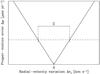Fig. 2 Schematic diagram showing how to quantify the sensitivity of the proper motion to a change in (read: measurement error of) radial velocity. A change in the radial velocity Δvr introduced before the backward solution leads to a certain (HTPM) proper-motion error Δμ. The linear dependence is commented on in Sect. 4.3. Since the magnitude of the proper-motion error does not depend on the sign but only on the magnitude of the radial-velocity variation, the sensitivity curve is symmetric with respect to the true radial velocity. The dashed horizontal line denotes the maximum perspective-acceleration-induced proper-motion error we are willing to accept in the HTPM proper motion. The distance Σ between the intersection points of the dashed horizontal line and the solid sensitivity curves determines the tolerance on the radial-velocity error.

4. The influence of radial velocity

4.1. Principle of the method

To quantify the influence of radial velocity on the HTPM proper motion for a star, we take the Hipparcos astrometric data (with epoch 1991.25) and the literature radial velocity from the XHIP catalogue (Sect. 2 – see Sect. 6.2 for stars without literature radial velocity) and use Eqs. (6), (7) to predict the star’s celestial position in 2014.5⁴, i.e., the mean epoch of the first intermediate-release Gaia astrometry. We then use backward solution, i.e., apply Eqs. (8), (8), to recover the proper motion from the given Hipparcos and Gaia positions on the sky, assuming that the parallax and time interval are known. Clearly, if the radial velocity (radial proper motion) used in the backward solution is identical to the radial velocity used in the forward propagation, the derived (HTPM) proper motion is essentially identical to the input (XHIP) proper motion (Table 1). However, by varying the radial velocity used for the backward solution away from the input value, the sensitivity of the HTPM proper motion on radial velocity is readily established. This sensitivity does not depend on the sign but only on the magnitude of the radial-velocity variation. Figure 2 schematically shows this idea. The abscissa shows the change in radial velocity, Δv_r, with respect to the input value used for the forward propagation. The ordinate shows Δμ (either Δμ_α or Δμ_δ), i.e., the difference between the input value of the proper motion (either μ_α or μ_δ) and the HTPM proper motion derived from the backward solution. The dashed horizontal line represents the maximum perspective-acceleration-induced proper-motion error that we are willing to accept. If we denote the radial-velocity interval spanned by the intersections between the dashed, horizontal threshold line and the two solid sensitivity curves by Σ (either Σ_α or Σ_δ), the tolerance on the radial-velocity standard error is easily expressed as $\mathrm{-}\frac{\mathrm{1}}{\mathrm{2}}\mathrm{\Sigma }\mathit{<}\mathrm{\Delta }{\mathit{v}}_{\mathit{r}}\mathit{<}\frac{\mathrm{1}}{\mathrm{2}}\mathrm{\Sigma }$. The question now is: what is the probability that the error in radial velocity (i.e., true radial velocity minus catalogue value) is smaller than $\mathrm{-}\frac{\mathrm{1}}{\mathrm{2}}\mathrm{\Sigma }$ or larger than $\frac{\mathrm{1}}{\mathrm{2}}\mathrm{\Sigma }$? 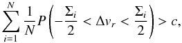Naturally, we want this probability to be smaller than a chosen threshold 1 − c, where c denotes the confidence level (for instance c = 0.6827 for a “1σ result”): $\mathit{P}\left(\mathrm{-}\frac{\mathrm{\Sigma }}{\mathrm{2}}\mathit{<}\mathrm{\Delta }{\mathit{v}}_{\mathit{r}}\mathit{<}\frac{\mathrm{\Sigma }}{\mathrm{2}}\right)\mathrm{=}\begin{array}{}\mathrm{˜}\\ \mathrm{\Phi }\end{array}\left[\frac{\mathrm{\Sigma }}{\mathrm{2}{\mathit{\sigma }}_{{\mathit{v}}_{\mathit{r}}}}\right]\mathit{>}\mathit{c,}$(10)where we have assumed that the error distribution for ΔV_r is a normal distribution with zero mean and variance ${\mathit{\sigma }}_{{\mathit{v}}_{\mathit{r}}}^{\mathrm{2}}$ and where $\begin{array}{}{}_{\mathrm{˜}}\\ \mathrm{\Phi }\end{array}\mathrm{\left(}\mathit{x}\mathrm{\right)}$ denotes the error function with argument x/$\sqrt{\mathrm{2}}$: $\begin{array}{}\mathrm{˜}\\ \mathrm{\Phi }\end{array}\mathrm{\left(}\mathit{x}\mathrm{\right)}\mathrm{=}\frac{\sqrt{\mathrm{2}}}{\sqrt{\mathit{\pi }}}{\mathrm{\int }}_{\mathrm{0}}^{\mathit{x}}\exp \left[\mathrm{-}\frac{\mathrm{1}}{\mathrm{2}}{\mathit{t}}^{\mathrm{2}}\right]\mathrm{d}\mathit{t}\mathrm{=}\mathrm{erf}\left(\frac{\mathit{x}}{\sqrt{\mathrm{2}}}\right)\mathrm{·}$(11)From Eq. (10), one can easily deduce: ${\mathit{\sigma }}_{{\mathit{v}}_{\mathit{r}}}\mathit{<}\frac{\mathrm{\Sigma }}{\mathrm{2}\begin{array}{}\mathrm{˜}\\ {\mathrm{\Phi }}^{-1}\end{array}\mathrm{\left(}\mathit{c}\mathrm{\right)}}\mathit{,}$(12)where $\begin{array}{}{\mathrm{˜}}_{}\\ {\mathrm{\Phi }}^{-1}\end{array}$ denotes the inverse of $\begin{array}{}{\mathrm{˜}}_{}\\ \mathrm{\Phi }\end{array}$ (e.g., $\begin{array}{}{}_{\mathrm{˜}}\\ {\mathrm{\Phi }}^{-1}\end{array}\mathrm{\left[}\mathrm{0.6827}\mathrm{\right]}\mathrm{=}\mathrm{1}$). For the “special case” c = 68.27%, Eq. (12) hence simplifies to ${\mathit{\sigma }}_{{\mathit{v}}_{\mathit{r}}}\mathit{<}\frac{\mathrm{1}}{\mathrm{2}}\mathrm{\Sigma }$.

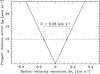Fig. 3 Sensitivity of the HTPM proper motion in right ascension to radial velocity for HIP 70890 (Proxima Centauri). The sensitivity is linear and has a value Cα = −74.59 μas yr-1 per km s-1 (Sect. 4.3). The dashed horizontal line indicates the maximum-tolerable perspective-acceleration-induced proper-motion error caused by an incorrect radial velocity. Since the expected HTPM standard error in right ascension is 97 μas yr-1 for this star, we set this threshold to 97/10 = 9.7 μas yr-1. This implies, for a confidence level c = 68.27%, that the maximum-acceptable radial-velocity standard error σvr for this object is $\frac{\mathrm{1}}{\mathrm{2}}\mathrm{\Sigma }\mathrm{=}\mathrm{0.13}$ km s-1.

4.2. Example for a real star

Figure 3 is similar to the schematic Fig. 2 but shows data for a real star, HIP 70890. This object, also known as Proxima Centauri (or α Cen C), is a nearby (ϖ = 772.33 ± 2.60 mas), fast-moving (μ_α = −3775.64 ± 1.52 mas yr^-1 and μ_δ = 768.16 ± 1.82 mas yr^-1) M6Ve flaring emission-line star which is known to have a significant perspective acceleration. HIP 70890 is actually one of the 21 stars in the Hipparcos catalogue for which the perspective acceleration was taken into account (ESA 1997a, Sect. 1.2.8). Figure 3 was constructed by comparing the input proper motion used in the forward propagation with the proper motion resulting from the backward solution while using a progressively differing radial velocity in the backward solution from the (fixed) value used in the forward propagation. The actual radial-velocity variation probed in this figure is small, only ± 0.5 km s^-1.

HIP 70890 is relatively faint (Hp = 10.7613 mag) and the expected HTPM proper-motion standard error is 97 μas yr^-1 (see Sect. 6.1 for details). If using a ten times lower threshold, i.e., 9.7 μas yr^-1, for the perspective-acceleration-induced proper-motion error caused by an incorrect radial velocity (see Sect. 6.1 for details), we find that Σ = 0.26 km s^-1. This implies, for a confidence level c = 68.27%, that the radial velocity should have been measured for this object with a standard error smaller than ${\mathit{\sigma }}_{{\mathit{v}}_{\mathit{r}}}\mathit{<}\frac{\mathrm{\Sigma }}{\mathrm{2}\begin{array}{}{}_{\mathrm{˜}}\\ {\mathrm{\Phi }}^{-1}\end{array}\mathrm{(}\mathit{c}\mathrm{=}\mathrm{0.6827}\mathrm{)}}\mathrm{=}\frac{\mathrm{1}}{\mathrm{2}}\mathrm{\Sigma }\mathrm{=}\mathrm{0.13}$ km s^-1. The literature radial velocity for this star is v_r = −22.40 ± 0.50 km s^-1 (with quality grade “B”; Sect. 2.2), which is not precise enough. New spectroscopic measurements are thus needed for this object to reduce the standard error by a factor ~4.

The discussion above has implicitly focused on the right-ascension proper-motion component μ_α, and the associated Σ_α, since the sensitivty of μ_δ is a factor ~4 less stringent for this star. It is generally sufficient to consider the most constraining case for a given star, i.e., either Σ_α or Σ_δ. Therefore, we drop from here on the subscript α and δ on Σ, implicitly meaning that it either refers to Σ_α or Σ_δ, depending on which one is largest. Typically, this is the largest proper-motion component, i.e., | μ_α | > | μ_δ | → Σ = Σ_α and | μ_α | < | μ_δ | → Σ = Σ_δ.

4.3. Derivation of the sensitivity

Figure 3 shows that the sensitivity of proper motion to radial velocity is linear. This can be understood by substitution of Eqs. (8), (8) in Eqs. (6), (7), after replacing v_r, as used in the forward propagation, by v_r + Δv_r in the backward solution: $\begin{array}{ccc}\mathrm{\Delta }{\mathit{\mu }}_{\mathit{\alpha }}& \mathrm{=}& {\mathit{\mu }}_{\mathit{\alpha }}\mathrm{-}\frac{\mathrm{1}}{\mathit{t}}[\mathrm{\Delta }{\mathit{\alpha }}^{\mathrm{\ast }}\mathrm{+}\mathrm{\Delta }{\mathit{\alpha }}^{\mathrm{\ast }}\left({\mathit{\mu }}_{\mathit{r}}\mathrm{+}\frac{\mathrm{\Delta }{\mathit{v}}_{\mathit{r}}}{\mathit{r}}\right)\mathit{t}\mathrm{-}\tan {\mathit{\delta }}_{\mathrm{0}}\mathrm{\Delta }{\mathit{\alpha }}^{\mathrm{\ast }}\mathrm{\Delta }\mathit{\delta }\\ & & \mathrm{+}\frac{\mathrm{3}{\cos }^{\mathrm{2}}{\mathit{\delta }}_{\mathrm{0}}\mathrm{-}\mathrm{1}}{\mathrm{6}{\cos }^{\mathrm{2}}{\mathit{\delta }}_{\mathrm{0}}}\mathrm{(}\mathrm{\Delta }{\mathit{\alpha }}^{\mathrm{\ast }}{\mathrm{)}}^{\mathrm{3}}\mathrm{-}\tan {\mathit{\delta }}_{\mathrm{0}}\mathrm{\Delta }{\mathit{\alpha }}^{\mathrm{\ast }}\mathrm{\Delta }\mathit{\delta }\left({\mathit{\mu }}_{\mathit{r}}\mathrm{+}\frac{\mathrm{\Delta }{\mathit{v}}_{\mathit{r}}}{\mathit{r}}\right)\mathit{t}]\\ & \mathrm{=}& {\mathit{\mu }}_{\mathit{\alpha }}\mathrm{-}\frac{\mathrm{1}}{\mathit{t}}\left[{\mathit{\mu }}_{\mathit{\alpha }}\mathit{t}\mathrm{+}\mathrm{\Delta }{\mathit{\alpha }}^{\mathrm{\ast }}\frac{\mathrm{\Delta }{\mathit{v}}_{\mathit{r}}}{\mathit{r}}\mathit{t}\mathrm{-}\tan {\mathit{\delta }}_{\mathrm{0}}\mathrm{\Delta }{\mathit{\alpha }}^{\mathrm{\ast }}\mathrm{\Delta }\mathit{\delta }\frac{\mathrm{\Delta }{\mathit{v}}_{\mathit{r}}}{\mathit{r}}\mathit{t}\right]\\ & \mathrm{=}& \begin{array}{}\underset{\mathrm{􏽼}0\mathrm{􏽻􏽺}0\mathrm{􏽽}}{\left[\frac{\mathrm{\Delta }{\mathit{\alpha }}^{\mathrm{\ast }}}{\mathit{r}}\mathrm{-}\tan {\mathit{\delta }}_{\mathrm{0}}\mathrm{\Delta }{\mathit{\alpha }}^{\mathrm{\ast }}\mathrm{\Delta }\mathit{\delta }\frac{\mathrm{1}}{\mathit{r}}\right]}\\ {\mathit{C}}_{\mathit{\alpha }}\end{array}\mathrm{\Delta }{\mathit{v}}_{\mathit{r}}\mathit{,}\end{array}$(13)which immediately shows Δμ_α ∝ Δv_r. A similar analysis for the sensitivity coefficient C_δ yields: $\mathrm{\Delta }{\mathit{\mu }}_{\mathit{\delta }}\mathrm{=}\begin{array}{}\underset{\mathrm{􏽼}0\mathrm{􏽻􏽺}0\mathrm{􏽽}}{\left[\frac{\mathrm{\Delta }\mathit{\delta }}{\mathit{r}}\mathrm{+}\frac{\mathrm{1}}{\mathrm{2}}\tan {\mathit{\delta }}_{\mathrm{0}}\mathrm{(}\mathrm{\Delta }{\mathit{\alpha }}^{\mathrm{\ast }}{\mathrm{)}}^{\mathrm{2}}\frac{\mathrm{1}}{\mathit{r}}\right]}\\ {\mathit{C}}_{\mathit{\delta }}\end{array}\mathrm{\Delta }{\mathit{v}}_{\mathit{r}}\mathit{.}$(14)The coefficients C_α and C_δ quantify the proper-motion-estimation error caused by a biased knowledge of v_r given measured displacements Δα ^∗  and Δδ. They can hence more formally be defined as the partial derivatives of μ_α and μ_δ from Eqs. (8) and (8) with respect to v_r with Δα ^∗  and Δδ kept constant: $\begin{array}{ccc}{\mathit{C}}_{\mathit{\alpha }}\mathrm{\equiv }\frac{\mathit{\partial }{\mathit{\mu }}_{\mathit{\alpha }}}{\mathit{\partial }{\mathit{v}}_{\mathit{r}}}\mathrm{=}\frac{\mathrm{1}}{\mathit{r}}\frac{\mathit{\partial }{\mathit{\mu }}_{\mathit{\alpha }}}{{\mathit{\mu }}_{\mathit{r}}}& \mathrm{=}& \frac{\mathrm{1}}{\mathit{r}}\left[\mathrm{\Delta }{\mathit{\alpha }}^{\mathrm{\ast }}\mathrm{-}\tan {\mathit{\delta }}_{\mathrm{0}}\mathrm{\Delta }{\mathit{\alpha }}^{\mathrm{\ast }}\mathrm{\Delta }\mathit{\delta }\right]\\ {\mathit{C}}_{\mathit{\delta }}\mathrm{\equiv }\frac{\mathit{\partial }{\mathit{\mu }}_{\mathit{\delta }}}{\mathit{\partial }{\mathit{v}}_{\mathit{r}}}\mathrm{=}\frac{\mathrm{1}}{\mathit{r}}\frac{\mathit{\partial }{\mathit{\mu }}_{\mathit{\delta }}}{{\mathit{\mu }}_{\mathit{r}}}& \mathrm{=}& \frac{\mathrm{1}}{\mathit{r}}\left[\mathrm{\Delta }\mathit{\delta }\mathrm{+}\frac{\mathrm{1}}{\mathrm{2}}\tan {\mathit{\delta }}_{\mathrm{0}}\mathrm{(}\mathrm{\Delta }{\mathit{\alpha }}^{\mathrm{\ast }}{\mathrm{)}}^{\mathrm{2}}\right]\mathit{.}\end{array}$Clearly, our relations confirm the well-known, classical result (e.g., Dravins et al. 1999, Eq. (4)) that perspective-acceleration-induced proper-motion errors are proportional to the product of the time interval, the parallax ϖ ∝ r^-1, the proper-motion components μ_α,δ, and the radial-velocity error Δv_r: Δμ_α,δ = C_α,δΔv_r = r^-1μ_α,δtΔv_r. Equations (13), (14) show that the perspective-acceleration-induced proper-motion error caused by a radial-velocity error does not depend on the radial velocity v_r itself but only on the error Δv_r. This may look counter-intuitive at first sight, since the proper motion itself is sensitive to the precise value of the radial velocity. The error in the proper motion, however, is sensitive only to the radial-velocity error. In other words, the slopes of the V-shaped wedge in Fig. 3 do not depend on the absolute but only on the relative labelling of the abscissa.

4.4. Taking measurement errors into account

So far, we ignored the measurement errors of the astrometric parameters α, δ, ϖ, μ_α, and μ_δ. A natural way to take these errors into account is by Monte-Carlo simulations: rather than deriving Σ once, namely based on the astrometric parameters contained in the XHIP catalogue, we calculate Σ a large number of times (typically N = 10   000), where in each run we do not use the catalogue astrometry but randomly distorted values drawn from normal distributions centred on the measured astrometry and with standard deviations equal to the standard errors of the astrometric parameters (denoted N(mean,variance)). We also randomly draw the radial velocity in each run from the normal probability distribution $\mathit{N}\mathrm{\left(}{\mathit{v}}_{\mathit{r}}\mathit{,}{\mathit{\sigma }}_{{\mathit{v}}_{\mathit{r}}}^{\mathrm{2}}\mathrm{\right)}$.

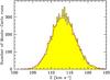Fig. 4 Histogram of the distribution of Σ in the N = 10   000 Monte-Carlo simulations for star HIP38 (ϖ = 23.64 ± 0.66 mas, so 3% relative error). The smooth, red curve is a Gaussian fit of the histogram; it provides a good representation.

The Monte-Carlo simulations yield N = 10   000 values for Σ; the interpretation of this distribution will be addressed in Sect. 5. Two representative examples of the distribution of Σ are shown in Figs. 4 and 5. The first distribution (Fig. 4, representing HIP38) is for a nearby star with a well-determined parallax: ϖ = 23.64 ± 0.66 mas, i.e., 3% relative parallax error. The smooth, red curve in Fig. 4 is a Gaussian fit of the histogram; it provides a good representation of the data. The second distribution (Fig. 5, representing HIP8) is for a distant star with a less well-determined parallax: ϖ = 4.98 ± 1.85 mas, i.e., 37% relative parallax error. This results in an asymmetric distribution of Σ with a tail towards large Σ values. This is easily explained since we essentially have $\mathrm{\Sigma }\mathrm{\propto }\mathrm{\Delta }{\mathit{v}}_{\mathit{r}}\mathrm{\propto }{\mathit{C}}_{\mathit{\alpha ,\delta }}^{-1}\mathrm{\propto }{\mathit{\varpi }}^{-1}$, meaning that the distribution of Σ reflects the probability distribution function of ϖ^-1 ∝ r. The latter is well-known (e.g., Kovalevsky 1998; Arenou & Luri 1999) for its extended tail towards large distances and its (light) contraction for small distances. The smooth, red curve in Fig. 5 is a Gaussian fit of the histogram; it provides an inadequate representation of the data. We will come back to this in Sect. 5.2.

To avoid dealing with (a significant number of) negative parallaxes in the Monte-Carlo simulations, we decided to ignore 11   171 entries with insignificant parallax measurements in the XHIP catalogue; these include 3920 entries with ϖ ≤ 0 and 7251 entries with 0 < ϖ/σ_ϖ ≤ 1 (recall that negative parallaxes are a natural outcome of the Hipparcos astrometric data reduction, e.g., Arenou et al. 1995). This choice does not influence the main conclusions of this paper: perspective-acceleration-induced HTPM proper-motion errors are significant only for nearby stars whereas negative and low-significance parallax measurements generally indicate large distances.

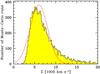Fig. 5 Histogram of the distribution of Σ in the N = 10   000 Monte-Carlo simulations for star HIP8 (ϖ = 4.98 ± 1.85 mas, so 37% relative error). The smooth, red curve is a Gaussian fit of the histogram; it provides a poor representation and does not account for the tail in the distribution.

5. Evaluation criteria

From the Monte-Carlo distribution of Σ (Sect. 4.4), we want to extract information to decide whether the radial velocity available in the literature is sufficiently precise or not. For this, we develop two evaluation criteria.

5.1. The Gaussian evaluation criterion

The first criterion, which we refer to as the Gaussian criterion, is based on Gaussian interpretations of probability distributions. It can be applied to all stars but, since we have seen that distant stars do not have a Gaussian Σ distribution, but rather a distribution with tails towards large Σ values (Fig. 5), the Gaussian criterion is unbiased, and hence useful, only for nearby stars. For these stars, the Monte-Carlo distribution of Σ is well described by a Gaussian function with mean μ_Σ and standard deviation σ_Σ (Fig. 4). The equations derived in Sect. 4.1 by ignoring astrometric errors are easily generalised by recognising that both the radial-velocity error and the distribution of Σ have Gaussian distributions, with standard deviations σ_vr and σ_Σ, respectively: $\mathit{P}\left(\mathrm{-}\frac{\mathrm{\Sigma }}{\mathrm{2}}\mathit{<}\mathrm{\Delta }{\mathit{v}}_{\mathit{r}}\mathit{<}\frac{\mathrm{\Sigma }}{\mathrm{2}}\right)\mathrm{=}\begin{array}{}\mathrm{˜}\\ \mathrm{\Phi }\end{array}\left[\frac{\mathrm{\Sigma }}{\mathrm{2}{\mathit{\sigma }}_{{\mathit{v}}_{\mathit{r}}}}\right]\mathit{>}\mathit{c}\mathit{.}$(17)generalises to: $\underset{\mathrm{\Sigma }\mathrm{=}\mathrm{-}\mathrm{\infty }}{\overset{\mathrm{\Sigma }\mathrm{=}\mathrm{\infty }}{\mathrm{\int }}}\frac{\mathrm{d\Sigma }}{\sqrt{\mathrm{2}\mathit{\pi }{\mathit{\sigma }}_{\mathrm{\Sigma }}^{\mathrm{2}}}}\exp \left[\mathrm{-}\frac{\mathrm{1}}{\mathrm{2}}{\left(\frac{\mathrm{\Sigma }\mathrm{-}{\mathit{\mu }}_{\mathrm{\Sigma }}}{{\mathit{\sigma }}_{\mathrm{\Sigma }}}\right)}^{\mathrm{2}}\right]\begin{array}{}\mathrm{˜}\\ \mathrm{\Phi }\end{array}\left[\frac{\mathrm{\Sigma }}{\mathrm{2}{\mathit{\sigma }}_{{\mathit{v}}_{\mathit{r}}}}\right]\mathit{>}\mathit{c}\mathit{.}$(18)Using Eq. (8.259.1) from Gradshteyn & Ryzhik (2007), Eq. (18) simplifies to: $\begin{array}{}\mathrm{˜}\\ \mathrm{\Phi }\end{array}\left[\frac{{\mathit{\mu }}_{\mathrm{\Sigma }}}{\sqrt{\mathrm{4}{\mathit{\sigma }}_{{\mathit{v}}_{\mathit{r}}}^{\mathrm{2}}\mathrm{+}{\mathit{\sigma }}_{\mathrm{\Sigma }}^{\mathrm{2}}}}\right]\mathit{>}\mathit{c,}$(19)which correctly reduces to Eq. (10) for the limiting, “error-free” case μ_Σ → Σ and σ_Σ → 0 in which the Gaussian distribution of Σ collapses into a delta function at μ_Σ = Σ, i.e., δ(Σ).

For the example of HIP 70890 discussed in Sect. 4.2, we find μ_Σ = 0.26 km s^-1 and σ_Σ = 0.000,89 km s^-1 so that, with σ_vr = 0.50 km s^-1, Eq. (19) returns c = 20.58%.

It is trivial, after re-arranging Eq. (19) to: ${\mathit{\sigma }}_{{\mathit{v}}_{\mathit{r}}}\mathit{<}\sqrt{\frac{{\mathit{\mu }}_{\mathrm{\Sigma }}^{\mathrm{2}}}{\mathrm{4}\mathrm{\left[}\begin{array}{}\mathrm{˜}\\ {\mathrm{\Phi }}^{-1}\end{array}\mathrm{\right(}\mathit{c}\mathrm{)}{\mathrm{]}}^{\mathrm{2}}}\mathrm{-}\frac{{\mathit{\sigma }}_{\mathrm{\Sigma }}^{\mathrm{2}}}{\mathrm{4}}}\mathit{,}$(20)to compute the required standard error of the radial velocity to comply with a certain confidence level c. For instance, if we require a c = 99.73% confidence level (for a “3σ result”), the radial-velocity standard error of HIP 70890 has to be 0.04 km s^-1. We finally note that Eq. (20) correctly reduces to Eq. (12) for the limiting, “error-free” case μ_Σ → Σ and σ_Σ → 0.

A limitation of Eq. (20) is that the argument of the square root has to be non-negative. This is physically easy to understand when realising that, in the Gaussian approximation, one has σ_Σ ≈ μ_Σ(σ_ϖ/ϖ) (see Sect. 4.4), so that: $\begin{array}{ccc}\frac{{\mathit{\mu }}_{\mathrm{\Sigma }}^{\mathrm{2}}}{\mathrm{4}\mathrm{\left[}\begin{array}{}\mathrm{˜}\\ {\mathrm{\Phi }}^{-1}\end{array}\mathrm{\right(}\mathit{c}\mathrm{)}{\mathrm{]}}^{\mathrm{2}}}\mathrm{-}\frac{{\mathit{\sigma }}_{\mathrm{\Sigma }}^{\mathrm{2}}}{\mathrm{4}}\mathrm{\ge }\mathrm{0}\mathrm{\to }\stackrel{}{{{\mathrm{\Phi }}^{-1}}_{\mathrm{˜}}}\mathrm{\left(}\mathit{c}\mathrm{\right)}\mathrm{\le }\frac{\mathit{\varpi }}{{\mathit{\sigma }}_{\mathit{\varpi }}}\mathrm{\to }\mathit{c}\mathrm{\le }\begin{array}{}\mathrm{˜}\\ \mathrm{\Phi }\end{array}\left[\frac{\mathit{\varpi }}{{\mathit{\sigma }}_{\mathit{\varpi }}}\right]\mathrm{·}& & \end{array}$(21)So, for instance, if a certain star has ϖ/σ_ϖ = 2 (a “2σ parallax”), the Gaussian methodology will only allow to derive the radial-velocity standard error σ_vr required to meet a confidence level c = 95.45% or lower.

5.2. The robust criterion

Since the Monte-Carlo distribution of Σ values is not Gaussianly distributed for distant stars (Fig. 5), the Gaussian criterion returns incorrect estimates; in fact, the estimates are not just incorrect but also biased since the Gaussian criterion systematically underestimates the mean value of Σ (i.e., μ_Σ) and hence systematically provides too conservative (small) estimates for σ_vr through Eq. (20). Rather than fitting a Gaussian function, we need a more robust estimator of the location and width of the Σ distribution than the Gaussian mean and standard deviation. This estimator is contained in the data itself and provides, what we call, the robust criterion.

Let us denote the individual values of Σ derived from the N = 10   000 Monte-Carlo simulations by Σ_i, with i = 1,...,N. Equation (18) is then readily generalised for arbitrary distributions of Σ to: $\sum _{\mathit{i}\mathrm{=}\mathrm{1}}^{\mathit{N}}\frac{\mathrm{1}}{\mathit{N}}\mathit{P}\left(\mathrm{-}\frac{{\mathrm{\Sigma }}_{\mathit{i}}}{\mathrm{2}}\mathit{<}\mathrm{\Delta }{\mathit{v}}_{\mathit{r}}\mathit{<}\frac{{\mathrm{\Sigma }}_{\mathit{i}}}{\mathrm{2}}\right)\mathrm{=}\sum _{\mathit{i}\mathrm{=}\mathrm{1}}^{\mathit{N}}\frac{\mathrm{1}}{\mathit{N}}\begin{array}{}\mathrm{˜}\\ \mathrm{\Phi }\end{array}\left[\frac{{\mathrm{\Sigma }}_{\mathit{i}}}{\mathrm{2}{\mathit{\sigma }}_{{\mathit{v}}_{\mathit{r}}}}\right]\mathit{>}\mathit{c}\mathit{.}$(22)The inverse relation generalising Eq. (20) by expressing σ_vr as function of c, required to determine the precision of the radial velocity required to comply with a certain confidence level c, is not analytical; we hence solve for it numerically.

The robust criterion generalises the Gaussian criterion. Both criteria return the same results for nearby stars which have a symmetric Gaussian distribution of Σ values. In general, therefore, the robust criterion is the prefered criterion for all stars, regardless of their distance.

6. Application of the evaluation criteria

6.1. Target proper-motion-error threshold

Before we can apply the Gaussian and robust criteria, we have to decide on a target proper-motion-error threshold for each star (i.e., the location of the dashed horizontal lines in Figs. 2 and 3). We adopt as a general rule that the maximum perspective-acceleration-induced HTPM proper-motion error caused by radial-velocity errors shall be an order of magnitude smaller than the predicted standard error of the HTPM proper motion itself (Sect. 7.2 discusses this choice in more detail). The latter quantity has been studied by Mignard (2009) and can be parametrised as: $\begin{array}{ccc}{\mathit{\sigma }}_{{\mathit{\mu }}_{\mathit{\alpha }}}\mathrm{\left[}\mathit{\mu }{\mathrm{as} \mathrm{yr}}^{-1}\mathrm{\right]}& \mathrm{=}& \mathrm{-}\mathrm{227.8}\mathrm{+}\mathrm{122.1}\mathit{H}\mathrm{-}\mathrm{20.39}{\mathit{H}}^{\mathrm{2}}\\ & \mathrm{+}& \\ {\mathit{\sigma }}_{{\mathit{\mu }}_{\mathit{\delta }}}\mathrm{\left[}\mathit{\mu }{\mathrm{as} \mathrm{yr}}^{-1}\mathrm{\right]}& \mathrm{=}& \mathrm{127.2}\mathrm{-}\mathrm{47.0}\mathit{H}\mathrm{+}\mathrm{8.30}{\mathit{H}}^{\mathrm{2}}\\ & \mathrm{-}& \mathrm{0.686}{\mathit{H}}^{\mathrm{3}}\mathrm{+}\mathrm{0.02581}{\mathit{H}}^{\mathrm{4}}\mathit{,}\end{array}$where H = max { 6.5,Hp [mag] }  with Hp the Hipparcos broad-band magnitude. These relations are shown in Fig. 6. The predicted HTPM standard errors include residual errors caused by the correction for the parallactic effect in the Gaia data (see footnote 1), the expected number and temporal distribution of the Gaia field-of-view transits for the Gaia nominal sky scanning law, and the expected location-estimation precision (“centroiding error”) of Gaia’s CCD-level data.

6.2. Stars without literature radial velocities

As already discussed in Sect. 2.2, the majority of stars in the XHIP catalogue do not have a literature radial velocity. These 71   563 objects are treated as stars with radial velocity, with three exceptions:

• 1.

  For each of theN = 10   000 Monte-Carlo simulations, the radial velocity is randomly taken from the full list of 46   392 radial velocites contained in the XHIP catalogue (Fig. 1). In practice, this choice does not influence our results since we are not sensitive to the absolute value of the radial velocity (Sect. 4.3). But at least in principle this choice means that there is a finite probability to assign a halo-star-like, i.e., large radial velocity in one (or more) of the Monte-Carlo runs. Regarding the HTPM Project, the best choice for stars without known radial velocity is to use v_r = −2.00 km s^-1, which is the median value of the distribution (recall that the mean equals −2.21 km s^-1).

• 2.

  For the Gaussian evaluation criterion (Sect. 5.1), we use σ_vr = 22.44 km s^-1 from the Gaussian fit to the distribution of all literature radial velocities. We also follow this recipe for the Gaussian criterion for the 1753 entries which do have a radial velocity but which do not have an associated standard error in the XHIP catalogue (this concerns 23 entries with quality grade “C” and 1730 entries with quality grade “D”). Clearly, this approach ignores the broad wings of the distribution visible in Fig. 1 as well as a small but finite number of halo stars and runaway stars with heliocentric radial velocities up to plus-or-minus several hundred km s^-1 (see Sect. 2.2). As a result, the Gaussian criterion systematically returns an overly optimistic (i.e., too large) confidence level c_Gauss for stars without literature radial velocity (Figs. 7 and 8). This bias comes in addition to the bias for distant stars for which the Gaussian criterion returns too conservative (small) estimates for σ_vr (Sect. 5.2).

• 3.

  For the robust evaluation criterion (Sect. 5.2), we do not make a priori assumptions except that the overall radial-velocity distribution of stars without known radial velocity is the same as the distribution of stars with literature radial velocity, including broad wings and “outliers”. We thus use Eq. (22) in the form: $\sum _{\mathit{i}\mathrm{=}\mathrm{1}}^{\mathit{N}}\frac{\mathrm{1}}{\mathit{N}}\mathit{P}\left(\mathrm{-}\frac{{\mathrm{\Sigma }}_{\mathit{i}}}{\mathrm{2}}\mathit{<}\mathrm{\Delta }{\mathit{v}}_{\mathit{r}}\mathit{<}\frac{{\mathrm{\Sigma }}_{\mathit{i}}}{\mathrm{2}}\right)\mathit{>}\mathit{c,}$(25)where the probability P that Δv_r is contained in the interval $\mathrm{[}\mathrm{-}\frac{\mathrm{1}}{\mathrm{2}}{\mathrm{\Sigma }}_{\mathit{i}}\mathit{,}\frac{\mathrm{1}}{\mathrm{2}}{\mathrm{\Sigma }}_{\mathit{i}}\mathrm{]}$ is calculated as the fraction of all stars with literature radial velocities in the XHIP catalogue which has ${\mathit{v}}_{\mathit{r}}\mathrm{\in }\mathrm{[}\mathrm{-}\frac{\mathrm{1}}{\mathrm{2}}{\mathrm{\Sigma }}_{\mathit{i}}\mathrm{+}{\mathit{v}}_{\mathit{r,}\mathrm{median}}\mathit{,}\frac{\mathrm{1}}{\mathrm{2}}{\mathrm{\Sigma }}_{\mathit{i}}\mathrm{+}{\mathit{v}}_{\mathit{r,}\mathrm{median}}\mathrm{]}$ (recall that the median radial velocity equals −2.00 km s^-1). We thus cater for the broad wings of the observed radial-velocity distribution (Figs. 1 and 7) as well as for the probability that the object is a (fast-moving) halo star, avoiding the bias in the Gaussian criterion discussed in the previous bullet.

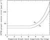Fig. 6 Predicted HTPM proper-motion error as function of the Hipparcos broad-band magnitude following Eqs. (23), (23). We require perspective-acceleration-induced proper-motion errors to be an order of magnitude smaller (factor of safety = FoS = 10; see Sect. 7.2).

6.3. Results of the application

We applied the Gaussian and robust criteria, as described in Sects. 5.1 and 5.2, respectively, to the XHIP catalogue. The results are presented in Table A.1 (Appendix A). The run time for N = 10   000 Monte-Carlo simulations is typically ~0.7 s per star and processing the full set of 117   955−11   171 = 106   784 XHIP entries with significant parallaxes (Sect. 4.4) hence takes about one day.

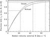Fig. 7 The fraction of stars with XHIP literature radial velocities which are contained in the radial-velocity interval [m − R,m + R]  as function of R, with m = −2.21 km s-1 the mean vr for the Gaussian criterion and m = −2.00 km s-1 the median vr for the robust criterion (Sects. 2.2 and 6.2). For the Gaussian criterion, we represent the histogram of literature radial velocities by a Gauss with standard deviation σ = 22.44 km s-1 (Fig. 1). The dashed lines represent the classical limits 1σ = 68.27%, 2σ = 95.45%, and 3σ = 99.73%. The fraction of stars with the robust criterion builds up more slowly as a result of the non-Gaussian broad wings as well as outliers representing halo and runaway stars. Since the Gaussian criterion ignores these features, it returns biased results for stars without literature radial velocity (see Sect. 6.3).

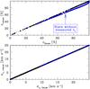Fig. 8 Comparison of the robust and Gaussian criteria for all stars with σϖ/ϖ better than 5%. The top panel compares the confidence levels while the bottom panel compares the radial-velocity standard errors σvr required to reach a confidence level c = 68.27%. The top panel shows two branches of data points: the linear, one-to-one branch corresponds to stars with a measured radial velocity, whereas the lower, curved branch corresponds to stars without measured radial velocity in the XHIP catalogue. As explained in Sect. 6.2, the latter objects suffer from a bias in the Gaussian confidence level cGauss.

Figures 9, 10 and Tables 2, 3 show the results for the confidence levels of the literature radial velocities contained in the XHIP catalogue. We find, not surprisingly since perspective-acceleration-induced proper-motion errors are relevant only for nearby, fast-moving stars – which are relatively rare – that the majority of stars have confidence levels exceeding c = 99.73%. This indicates that, at the c = 99.73% confidence level, the available radial velocity is sufficiently precise or, for stars without literature radial velocity, that the absence of a literature radial velocity, and hence the assumption v_r = −2.00 km s^-1 for the robust criterion or v_r = −2.21 km s^-1 for the Gaussian criterion, is acceptable. This holds for more than 100   000 stars using the robust criterion (Table 3) and more than 85   000 stars using the Gaussian criterion (Table 2). The large difference between the two criteria does not come unexpectedly:

• 1.

  We already argued in Sect. 5.2 that the Gaussiancriterion is biased for distant stars, with distant meaning that theparallax probability distribution has an associated asymmetricdistance probability distribution. For such stars, the Gaussiancriterion systematically underestimates the mean value ofΣ and hence returns too conservative (small) values for σ_vr for a given value of the confidence level c and too pessimistic (small) values of c for a given value of σ_vr.

• 2.

  We already argued in Sect. 6.2 that the Gaussian criterion is biased for stars without literature radial velocity. For such stars, the Gaussian criterion systematically returns too optimistic (large) values of the confidence level c since it ignores the broad wings of the observed distribution of radial velocities (Figs. 1, 7, and 8) and also ignores the probability that the object is actually a halo (or runaway) star.

The robust criterion does not suffer from these biases and hence, being more reliable, is prefered for all stars. The Gaussian criterion, nonetheless, provides a useful and also easily interpretable reference test case and we hence decided to retain it. Figure 8 shows that, for nearby stars with literature radial velocities, the Gaussian and robust criteria return equivalent results.

For a small but non-negligible number of stars, Table 3 indicates insatisfactory results: 206 stars have a confidence level c < 68.27%: 97 of these do have a literature radial velocity in the XHIP catalogue but one which is insufficiently precise. The remaining 109 stars do not have a spectroscopically measured radial velocity (at least not one contained in the XHIP catalogue). New spectroscopy is hence required for these stars to guarantee a confidence level of at least 68.27%. For increased confidence levels, the numbers obviously increase: if requiring a c = 99.73% confidence level for all objects, for instance, the number of “problem stars” increases to 6562, split into 382 with insufficiently-precise known radial velocity and 6180 without known radial velocity. We conclude that, depending on the confidence level one wants to achieve, hundreds to thousands of stars need to be spectroscopically re-measured.

Figure 11 shows the robust confidence level versus Hp magnitude. One can see that the typical star which needs a high-priority spectroscopic measurement (i.e., c < 68.27%) has Hp in the range 8–12 mag. Figure 12 shows the radial-velocity precision required to reach c = 68.27% (computed with the robust criterion) versus magnitude. Precisions vary drastically, from very stringent values well below 1 km s^-1 to very loose values, up to several tens of km s^-1.

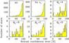
Fig. 9 Histograms of the Gaussian confidence level c from Sect. 5.1 for all stars combined, stars without measured radial velocity, and stars with measured radial velocity as function of radial-velocity quality grade Qvr (see Sect. 2.2 and Appendix A). The vast majority of objects have c > 95.45% (see Table 2); they have been omitted from the histograms to improve their legibility.

Fig. 10 As Fig. 9, but for the robust criterion from Sect. 5.2.

7. Discussion

7.1. HTPM bright limit

The HTPM catalogue will contain the intersection of the Hipparcos and Gaia catalogues. Whereas the Hipparcos catalogue (ESA 1997b), which contains 117 955 entries with astrometry (and 118 218 entries in total), is complete to at least V = 7.3 mag (ESA 1997a, Sect. 1.1), the Gaia catalogue will be incomplete at the bright end. Gaia’s bright limit is G = 5.7 mag (de Bruijne 2012), where G is the white-light, broad-band Gaia magnitude, which is linked to the Hipparcos Hp, the Cousins I, and the Johnson V magnitudes through (Jordi et al. 2010): $\begin{array}{ccc}\mathit{G}\mathrm{-}\mathit{V}& \mathrm{=}& \mathrm{-}\mathrm{0.0447}\mathrm{-}\mathrm{0.1634}\mathrm{(}\mathit{Hp}\mathrm{-}\mathit{I}\mathrm{)}\\ & \mathrm{+}& \mathrm{0.0331}\mathrm{(}\mathit{Hp}\mathrm{-}\mathit{I}{\mathrm{)}}^{\mathrm{2}}\mathrm{-}\mathrm{0.0371}\mathrm{(}\mathit{Hp}\mathrm{-}\mathit{I}{\mathrm{)}}^{\mathrm{3}}\mathit{.}\end{array}$(26)For stars in the Hipparcos catalogue, the colour G − Hp ranges between −0.5 and 0.0 mag, with a mean value of −0.3 mag. This means that G = 5.7 mag corresponds roughly to Hp ≈ 6.0 mag. In practice, therefore, we are not concerned with the brightest ~4509 stars in the sky. The expected number of HTPM-catalogue entries is therefore ~117   955−4509 ≈ 113   500. The number of entries with significant parallax measurements equals 117   955−11   171 = 106   784, of which 106   784−4468 = 102   316 have G > 5.7 mag.

7.2. Proper-motion-error threshold

For both the Gaussian and the robust criteria, we adopt, somewhat arbitrarily, the rule that the perspective-acceleration-induced HTPM proper-motion error caused by radial-velocity errors shall be an order of magnitude smaller than the predicted standard error of the HTPM proper motion itself (Sect. 6.1). The adopted Factor of Safety (FoS) is hence 10. Some readers may find that this “rule” is too stringent. Unfortunately, there is no easy (linear) way to scale our results if the reader wants to adopt a different value for the FoS. Clearly, the value of Σ in each Monte-Carlo run is linearly proportional to the FoS (see, for instance, Fig. 2). However, the robust confidence level c_robust and the radial-velocity standard error σ_vr required to meet a certain value of c_robust do not linearly depend on Σ but on the properties of the, in general asymmetric, distribution of the N = 10   000 values of Σ resulting from the Monte-Carlo processing. To zeroth order, however, one can assume a linear relationship between σ_vr and Σ and hence the adopted FoS, as is also apparent from the “error-free” criterion ${\mathit{\sigma }}_{{\mathit{v}}_{\mathit{r}}}\mathit{<}\frac{\mathrm{1}}{\mathrm{2}}\mathrm{\Sigma }$ derived for c = 68.27% in Sect. 4.1. This is in particular a fair approximation for small variations around the default value (FoS = 10) in combination with nearby stars, which are most interesting because these are most sensitive to perspective acceleration. The Monte-Carlo distribution of Σ values for these objects is generally well behaved, i.e., symmetric and with σ_ϖ ≪ ϖ and hence σ_Σ ≪ μ_Σ (see, for instance, Fig. 4; see also Sect. 5.1). Figure 13 shows, as an example for the nearby star HIP 57367 (see Table 4), how σ_vr (required for c_robust = 68.27%) and c_robust vary as function of the FoS. Linear scaling around the default FoS = 10 provides a decent approximation, at least over the range 10/2 = 5 < FoS < 20 = 10 × 2.

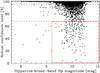Fig. 11 Robust confidence level c versus Hipparcos broad-band magnitude. The red box in the bottom-right corner denotes the approximate area for high-priority follow-up spectroscopy: stars with confidence level c < 68.27% and mag. The latter restriction roughly reflects Gaia’s – and hence HTPM’s – bright limit (Sect. 7.1).

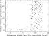Fig. 12 Radial-velocity precision (standard error) for stars with robust confidence level c < 68.27% required to upgrade their confidence level to c = 68.27%.

7.3. Number of Monte-Carlo simulations

To take measurement errors in the XHIP astrometry and literature radial velocities into account, we adopt a Monte-Carlo scheme in which we run a number N of Monte-Carlo simulations for each star in which we randomly vary the astrometric and spectroscopic data within their respective error bars (see Sect. 4.4). Clearly, the higher the value of N is, the more reliable the results are. We adopted N = 10   000 as a practical compromise, resulting in an acceptable, typical run time of ~1 s per star as well as smooth distributions of Σ (see, for instance, Fig. 4 or 5). To investigate the repeatability and hence reliability of our robust confidence levels c_robust and radial-velocity errors σ_vr, we have repeated the entire processing with N = 10   000 runs 100 times for the 206 stars with c_robust < 68.27% (Sect. 6.3) and find that the typical variation of the confidence level and the radial-velocity error, quantified by the standard deviation divided by the average of the distribution containing the 100 results, is less than 0.1% and 0.2%, respectively; the maximum variation among the 206 objects is found for HIP 107711 and amounts to 0.5% and 0.6%, respectively.

7.4. High-priority and challenging stars

Table 4 shows the ten stars with the lowest robust confidence level. These stars are the highest-priority targets for spectroscopic follow-up. Nine of the ten entries do have a literature radial velocity but one which is insufficiently precise. The highest-priority object (HIP 57367) does not yet have a spectroscopic radial velocity and needs a measurement with a standard error better than 1 km s^-1. For this particular object, this challenge seems insurmountable since it is one of the 20 white dwarfs with Hipparcos astrometry (Vauclair et al. 1997), objects for which it is notoriously difficult to obtain – even low-precision – spectroscopic radial velocities.

Table 5 shows the ten stars, among the subset of stars with unacceptably-low robust confidence level (c_robust < 68.27%), with the smallest radial-velocity standard errors required to raise the robust confidence level to c_robust = 68.27%. Since c_robust < 68.27%, these stars do clearly need spectroscopic follow-up. However, the radial-velocity standard errors reach values as small as 0.04 km s^-1, which is a real challenge, not only in terms of the required signal-to-noise ratio of the spectroscopic data but also in view of the definition of the radial-velocity zero-point at this level of precision (Crifo et al. 2010) as well as potential systematic errors in the radial velocities, both with instrumental origin and with astrophysical causes such as radial-velocity differences between various absorption lines etc. (see Lindegren & Dravins 2003, for a detailed discussion of this and other effects).

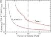Fig. 13 Dependence, for HIP 57367 (see Table 4), of σvr (required to reach crobust = 68.27%) and the robust confidence level crobust on the Factor of Safety (FoS), i.e., the minimum factor between the predicted HTPM standard error and the perspective-acceleration-induced HTPM proper-motion error caused by radial-velocity errors. The default FoS value adopted in this study is 10. The object is representative for a nearby star with a well-determined parallax. The straight, red lines indicate linear scaling relations starting from the default value FoS = 10.

Table 2 in Dravins et al. (1999) shows the top-39 of stars in the Gliese & Jahreiss (1995) preliminary third catalogue of nearby stars ranked according to the magnitude of the perspective acceleration (which is propertional to ϖμ). Similarly, Table 1.2.3 in ESA (1997a) shows the top-21 of stars in the Hipparcos catalogue for which the magnitude of the perspective acceleration is significant enough to have been taken into account in the Hipparcos data processing (the accumulated effect on position is proportional to ϖμ | v_r | ). On the contrary, the top-10 Tables 4 and 5 have been constructed based on the sensitivity of the perspective acceleration to radial-velocity errors (Sect. 4.3) and the associated confidence level of the available literature radial velocity. Hence, although there is a significant overlap of stars between the various tables, they are understandably not identical.

7.5. Object-by-object analyses and other literature sources

In general, and in particular for the most interesting, delicate, or border cases, it will be useful to perform a more in-depth literature search for and study of radial velocities and other available data before embarking on ground-based spectroscopy. For instance, we found a SIMBAD note on the Hipparcos catalogue (ESA 1997a,b, CDS catalogue I/239) for HIP 114110 (c_robust = 71.23%) and HIP 114176 (c_robust = 60.00%) that they are non-existing objects: “HIP 114110 (observed with HIP 14113⁵) and HIP 114176 (observed with HIP 114177) are noted as probable measurements of scattered light from a nearby bright star. The non-reality of 114110 and 114176 (traced to fictitious entries in the WDS and INCA) has been confirmed by MMT observations reported by Latham (priv. comm., 8 May 1998), and confirmed by inspection of the DSS [J. L. Falin, 12 May 1998]”. In addition, the completeness and coverage level of the XHIP radial-velocity compilation is not known. We did query SIMBAD as well as the Geneva-Copenhagen-Survey (GCS, CORAVEL) database (Nordström et al. 2004, CDS catalogue V/117) and the RAVE database (Siebert et al. 2011, CDS catalogue III/265, with 77,461 entries with a mean precision of 2.3 km s^-1) for radial velocities for the 109 stars without XHIP radial velocity and with confidence level below 68.27% but did not find new data. Unfortunately, the treasure contained in the full CORAVEL database (45 263 late-type Hipparcos stars with precisions below 1 km s^-1), the public release of which was announced in Udry et al. (1997) to be before the turn of the previous millennium, remains a mystery to date. All in all, dedicated studies for individual objects might pay off by reducing the needs for spectroscopic follow-up.

7.6. Urgency of the spectroscopic follow-up

Mignard (2009) already acknowledges that, since the perspective-acceleration-induced proper-motion error can be calculated as function of radial velocity, a factor – effectively the sensitivity coefficients C_α and C_δ from Eqs. (13), (14) in Sect. 4.3 – can be published to correct the HTPM proper motion for a particular star a posteriori when v_r becomes known or when a more precise v_r becomes available. Therefore, both the reference radial velocity v_r and parallax ϖ used in the HTPM derivation will be published together with the proper-motion values themselves. This means that the spectroscopic follow-up identified in this paper is not time-critical: the HTPM catalogue can and will be published in any case, even if not all required spectroscopic follow-up has been completed. Of course, the implication for stars without the required radial-velocity knowledge will be that their HTPM proper motions will include a (potentially) significant perspective-acceleration-induced error.

8. Conclusions

We have conducted a study of the requirements for the availability of radial velocities for the Hundred-Thousand-Proper-Motion (HTPM) project (Mignard 2009). This unique project will combine Hipparcos astrometry from 1991.25 with early-release Gaia astrometry (~2014.5) to derive long-time-baseline and hence precise proper motions. For the nearest, fast-moving stars, the perspective acceleration of the objects on the sky requires the presence of radial velocities for the derivation of the proper motions. We have quantitatively determined, for each star in the Hipparcos catalogue, the precision of the radial velocity that is required to ensure that the perspective-acceleration-induced error in the HTPM proper motion caused by the radial-velocity error is negligible. Our method takes the Hipparcos measurement errors into account and allows the user to specify his/her own prefered confidence level (e.g., 68.27%, 95.45%, or 99.73%). The results are available in Table A.1 (Appendix A). We have compared the radial-velocity-precision requirements to the set of 46   392 radial velocities contained in the XHIP compilation catalogue (Anderson & Francis 2012) and find that, depending on the confidence level one wants to achieve, hundreds to thousands of stars require spectroscopic follow-up. The highest-priority targets are 206 objects with a confidence level below 68.27%; 97 of them have a known but insufficiently precise radial velocity while the remaining 109 objects have no literature radial velocity in the XHIP compilation catalogue at all. The typical brightness of the objects requiring their radial velocity to be (re-)determined is Hp ≈ 8−12 mag and the radial-velocity precisions vary drastically, ranging from 0.04 km s^-1 for the most extreme case (HIP 87937, also known as Barnard’s star) to a few tens of km s^-1. With only few exceptions, the spectral types are K and M; 73% of them are in the south. Gaia’s Radial-Velocity Spectrometer (RVS; Cropper & Katz 2011) will deliver radial velocities for all stars in the HTPM catalogue with Gaia-end-of-mission precisions below a few km s^-1 (and ~10 km s^-1 for early-type stars; de Bruijne 2012); however, these performances require full calibration of the instrument and data and hence will most likely only be reached in the final Gaia data release, at which time the HTPM proper motions will be superseded by the Gaia proper motions. Fortunately, the spectroscopic follow-up is not time-critical in the sense that the HTPM catalogue will be published with information (sensitivity coefficients and reference parallax and radial velocity) to correct the proper motions a posteriori when (improved) radial velocities become available.

We finally note that the spectroscopic follow-up requirements for the HTPM proper motions quantified in this work will be dwarfed by the requirements coming from the end-of-mission Gaia proper motions, to be released around ~2021: for instance for the stars in the HTPM catalogue, for which the HTPM proper-motion standard errors are 30−190 μas yr^-1, the Gaia proper-motion standard errors reach the bright-star floor around 3–4 μas yr^-1 (de Bruijne 2012), which means that the spectroscopic requirements for the correction of perspective acceleration in the Gaia astrometry, with a 5-year baseline, will be a factor ~2–10 more demanding.

Acknowledgments

It is a pleasure to thank Mark Cropper for discussions about radial-velocity surveys and the referee, François Mignard, for his constructive criticism which helped to improve our statistical methodology. This research has made use of the SIMBAD database and VizieR catalogue access tool, both operated at the Centre de Données astronomiques de Strasbourg (CDS), and of NASA’s Astrophysics Data System (ADS).

References

Appendix A: The results data file

Table A.1 describes the results data file, which is available at the CDS.

All Tables

All Figures

	Fig. 1 Distribution of all 46 392 radial velocities contained in the XHIP catalogue. The smooth, red curve fits the histogram with a Gaussian normal distribution. The best-fit mean and standard deviation are μ = −2.21 km s-1 and σ = 22.44 km s-1, respectively.
In the text

Fig. 2 Schematic diagram showing how to quantify the sensitivity of the proper motion to a change in (read: measurement error of) radial velocity. A change in the radial velocity Δvr introduced before the backward solution leads to a certain (HTPM) proper-motion error Δμ. The linear dependence is commented on in Sect. 4.3. Since the magnitude of the proper-motion error does not depend on the sign but only on the magnitude of the radial-velocity variation, the sensitivity curve is symmetric with respect to the true radial velocity. The dashed horizontal line denotes the maximum perspective-acceleration-induced proper-motion error we are willing to accept in the HTPM proper motion. The distance Σ between the intersection points of the dashed horizontal line and the solid sensitivity curves determines the tolerance on the radial-velocity error.

In the text

Fig. 3 Sensitivity of the HTPM proper motion in right ascension to radial velocity for HIP 70890 (Proxima Centauri). The sensitivity is linear and has a value Cα = −74.59 μas yr-1 per km s-1 (Sect. 4.3). The dashed horizontal line indicates the maximum-tolerable perspective-acceleration-induced proper-motion error caused by an incorrect radial velocity. Since the expected HTPM standard error in right ascension is 97 μas yr-1 for this star, we set this threshold to 97/10 = 9.7 μas yr-1. This implies, for a confidence level c = 68.27%, that the maximum-acceptable radial-velocity standard error σvr for this object is $\frac{\mathrm{1}}{\mathrm{2}}\mathrm{\Sigma }\mathrm{=}\mathrm{0.13}$ km s-1.

In the text

	Fig. 4 Histogram of the distribution of Σ in the N = 10   000 Monte-Carlo simulations for star HIP38 (ϖ = 23.64 ± 0.66 mas, so 3% relative error). The smooth, red curve is a Gaussian fit of the histogram; it provides a good representation.
In the text

	Fig. 5 Histogram of the distribution of Σ in the N = 10   000 Monte-Carlo simulations for star HIP8 (ϖ = 4.98 ± 1.85 mas, so 37% relative error). The smooth, red curve is a Gaussian fit of the histogram; it provides a poor representation and does not account for the tail in the distribution.
In the text

	Fig. 6 Predicted HTPM proper-motion error as function of the Hipparcos broad-band magnitude following Eqs. (23), (23). We require perspective-acceleration-induced proper-motion errors to be an order of magnitude smaller (factor of safety = FoS = 10; see Sect. 7.2).
In the text

Fig. 7 The fraction of stars with XHIP literature radial velocities which are contained in the radial-velocity interval [m − R,m + R]  as function of R, with m = −2.21 km s-1 the mean vr for the Gaussian criterion and m = −2.00 km s-1 the median vr for the robust criterion (Sects. 2.2 and 6.2). For the Gaussian criterion, we represent the histogram of literature radial velocities by a Gauss with standard deviation σ = 22.44 km s-1 (Fig. 1). The dashed lines represent the classical limits 1σ = 68.27%, 2σ = 95.45%, and 3σ = 99.73%. The fraction of stars with the robust criterion builds up more slowly as a result of the non-Gaussian broad wings as well as outliers representing halo and runaway stars. Since the Gaussian criterion ignores these features, it returns biased results for stars without literature radial velocity (see Sect. 6.3).

In the text

Fig. 8 Comparison of the robust and Gaussian criteria for all stars with σϖ/ϖ better than 5%. The top panel compares the confidence levels while the bottom panel compares the radial-velocity standard errors σvr required to reach a confidence level c = 68.27%. The top panel shows two branches of data points: the linear, one-to-one branch corresponds to stars with a measured radial velocity, whereas the lower, curved branch corresponds to stars without measured radial velocity in the XHIP catalogue. As explained in Sect. 6.2, the latter objects suffer from a bias in the Gaussian confidence level cGauss.

In the text

	Fig. 9 Histograms of the Gaussian confidence level c from Sect. 5.1 for all stars combined, stars without measured radial velocity, and stars with measured radial velocity as function of radial-velocity quality grade Qvr (see Sect. 2.2 and Appendix A). The vast majority of objects have c > 95.45% (see Table 2); they have been omitted from the histograms to improve their legibility.
In the text

	Fig. 10 As Fig. 9, but for the robust criterion from Sect. 5.2.
In the text

	Fig. 11 Robust confidence level c versus Hipparcos broad-band magnitude. The red box in the bottom-right corner denotes the approximate area for high-priority follow-up spectroscopy: stars with confidence level c < 68.27% and mag. The latter restriction roughly reflects Gaia’s – and hence HTPM’s – bright limit (Sect. 7.1).
In the text

	Fig. 12 Radial-velocity precision (standard error) for stars with robust confidence level c < 68.27% required to upgrade their confidence level to c = 68.27%.
In the text

Fig. 13 Dependence, for HIP 57367 (see Table 4), of σvr (required to reach crobust = 68.27%) and the robust confidence level crobust on the Factor of Safety (FoS), i.e., the minimum factor between the predicted HTPM standard error and the perspective-acceleration-induced HTPM proper-motion error caused by radial-velocity errors. The default FoS value adopted in this study is 10. The object is representative for a nearby star with a well-determined parallax. The straight, red lines indicate linear scaling relations starting from the default value FoS = 10.

In the text

References

- Anderson, E., & Francis, C. 2012, Astron. Lett., 38, 331 [NASA ADS] [CrossRef] [Google Scholar]
- Antoja, T., Figueras, F., Romero-Gómez, M., et al. 2011, MNRAS, 418, 1423 [NASA ADS] [CrossRef] [Google Scholar]
- Arenou, F., & Luri, X. 1999, in Harmonizing Cosmic Distance Scales in a Post-Hipparcos Era, eds. D. Egret, & A. Heck, ASP Conf. Ser., 167, 13 [Google Scholar]
- Arenou, F., Lindegren, L., Froeschle, M., et al. 1995, A&A, 304, 52 [NASA ADS] [Google Scholar]
- Bailer-Jones, C. A. L. 2010, MNRAS, 403, 96 [NASA ADS] [CrossRef] [Google Scholar]
- Crifo, F., Jasniewicz, G., Soubiran, C., et al. 2010, A&A, 524, A10 [NASA ADS] [CrossRef] [EDP Sciences] [Google Scholar]
- Cropper, M., & Katz, D. 2011, in EAS Pub. Ser., 45, 181 [Google Scholar]
- de Bruijne, J. H. J. 1999, MNRAS, 310, 585 [NASA ADS] [CrossRef] [Google Scholar]
- de Bruijne, J. H. J. 2012, Ap&SS, 341, 31 [NASA ADS] [CrossRef] [Google Scholar]
- de Bruijne, J. H. J., Hoogerwerf, R., & de Zeeuw, P. T. 2001, A&A, 367, 111 [NASA ADS] [CrossRef] [EDP Sciences] [Google Scholar]
- de Bruijne, J. H. J., Kohley, R., & Prusti, T. 2010, in SPIE Conf. Ser., 7731 [Google Scholar]
- Delhaye, J. 1965, in Galactic Structure, eds. A. Blaauw, & M. Schmidt, 61 [Google Scholar]
- Dravins, D., Lindegren, L., & Madsen, S. 1999, A&A, 348, 1040 [NASA ADS] [Google Scholar]
- Elias, F., Alfaro, E. J., & Cabrera-Caño, J. 2006, AJ, 132, 1052 [NASA ADS] [CrossRef] [Google Scholar]
- ESA 1997a, The Hipparcos and TYCHO catalogues, Astrometric and photometric star catalogues derived from the ESA Hipparcos Space Astrometry Mission, ESA SP, 1200 [Google Scholar]
- ESA 1997b, VizieR Online Data Catalog, I/239 [Google Scholar]
- Eyer, L., Suveges, M., Dubath, P., et al. 2011, in EAS Pub. Ser., 45, 161 [Google Scholar]
- Gliese, W., & Jahreiss, H. 1995, VizieR Online Data Catalog, V/70 [Google Scholar]
- Gómez, F. A., Helmi, A., Brown, A. G. A., & Li, Y.-S. 2010, MNRAS, 408, 935 [NASA ADS] [CrossRef] [Google Scholar]
- Gradshteyn, I. S., & Ryzhik, M. 2007, Tables of Integrals, Series, and Product (7th edition), eds. A. Jeffrey, & D. Zwillinger (Academic Press) [Google Scholar]
- Høg, E., Fabricius, C., Makarov, V. V., et al. 2000a, VizieR Online Data Catalog, I/259 [Google Scholar]
- Høg, E., Fabricius, C., Makarov, V. V., et al. 2000b, A&A, 355, L27 [NASA ADS] [Google Scholar]
- Hoogerwerf, R., de Bruijne, J. H. J., & de Zeeuw, P. T. 2001, A&A, 365, 49 [NASA ADS] [CrossRef] [EDP Sciences] [Google Scholar]
- Jordi, C., Gebran, M., Carrasco, J. M., et al. 2010, A&A, 523, A48 [NASA ADS] [CrossRef] [EDP Sciences] [Google Scholar]
- Joshi, Y. C. 2007, MNRAS, 378, 768 [NASA ADS] [CrossRef] [Google Scholar]
- Katz, D., Cropper, M., Meynadier, F., et al. 2011, in EAS Pub. Ser., 45, 194 [Google Scholar]
- Kordopatis, G., Recio-Blanco, A., de Laverny, P., et al. 2011, A&A, 535, A106 [NASA ADS] [CrossRef] [EDP Sciences] [Google Scholar]
- Kovalevsky, J. 1998, A&A, 340, L35 [NASA ADS] [Google Scholar]
- Lindegren, L., & Dravins, D. 2003, A&A, 401, 1185 [NASA ADS] [CrossRef] [EDP Sciences] [Google Scholar]
- Lindegren, L., Babusiaux, C., Bailer-Jones, C., et al. 2008, in IAU Symp., 248, eds. W. J. Jin, I. Platais, & M. A. C. Perryman, 217 [Google Scholar]
- Lindegren, L., Lammers, U., Hobbs, D., et al. 2012, A&A, 538, A78 [NASA ADS] [CrossRef] [EDP Sciences] [Google Scholar]
- Liu, J.-C., Zhu, Z., & Hu, B. 2011, Res. Astron. Astrophys., 11, 1074 [NASA ADS] [CrossRef] [Google Scholar]
- Madsen, S., Dravins, D., & Lindegren, L. 2002, A&A, 381, 446 [NASA ADS] [CrossRef] [EDP Sciences] [Google Scholar]
- Mignard, F. 2009, Gaia Data Processing and Analysis Consortium (DPAC) technical note Gaia-C3-TN-OCA-FM-040, The Hundred-Thousand-Proper-Motion project [Google Scholar]
- Mignard, F., & Klioner, S. A. 2010, in ed. S. A. Klioner, P. K. Seidelmann, & M. H. Soffel, IAU Symp., 261, 306 [Google Scholar]
- Mouret, S. 2011, Phys. Rev. D, 84, 122001 [NASA ADS] [CrossRef] [Google Scholar]
- Nordström, B., Mayor, M., Andersen, J., et al. 2004, A&A, 418, 989 [NASA ADS] [CrossRef] [EDP Sciences] [Google Scholar]
- Oort, J. H. 1927, Bull. Astron. Inst. Netherlands, 3, 275 [NASA ADS] [Google Scholar]
- Perryman, M. 2009, Astronomical Applications of Astrometry: Ten Years of Exploitation of the Hipparcos Satellite Data, ed. M. Perryman (Cambridge University Press) [Google Scholar]
- Perryman, M. A. C., Lindegren, L., Kovalevsky, J., et al. 1997, A&A, 323, L49 [NASA ADS] [Google Scholar]
- Perryman, M. A. C., de Boer, K. S., Gilmore, G., et al. 2001, A&A, 369, 339 [NASA ADS] [CrossRef] [EDP Sciences] [Google Scholar]
- Pourbaix, D. 2008, in IAU Symp. ed. W. J. Jin, I. Platais, & M. A. C. Perryman, 248, 59 [Google Scholar]
- Röser, S., Schilbach, E., Schwan, H., et al. 2008, A&A, 488, 401 [NASA ADS] [CrossRef] [EDP Sciences] [Google Scholar]
- Röser, S., Demleitner, M., & Schilbach, E. 2010, AJ, 139, 2440 [NASA ADS] [CrossRef] [Google Scholar]
- Schönrich, R., & Binney, J. 2009, MNRAS, 399, 1145 [NASA ADS] [CrossRef] [Google Scholar]
- Schönrich, R., Binney, J., & Dehnen, W. 2010, MNRAS, 403, 1829 [NASA ADS] [CrossRef] [Google Scholar]
- Schwarzschild, K. 1907, Nachrichten von der Gesellschaft der Wissenschaften zu Göttingen, 614 [Google Scholar]
- Seeliger, H. 1900, Astron. Nachr., 154, 65 [NASA ADS] [CrossRef] [Google Scholar]
- Siebert, A., Williams, M. E. K., Siviero, A., et al. 2011, AJ, 141, 187 [NASA ADS] [CrossRef] [Google Scholar]
- Sozzetti, A. 2011, in EAS Publ. Ser., 45, 273 [Google Scholar]
- Tanga, P., Hestroffer, D., Delbò, M., et al. 2008, Planet. Space Sci., 56, 1812 [Google Scholar]
- Udry, S.,Mayor, M.,Andersen, J., et al. 1997, in Hipparcos – Venice ’97, eds. R. M. Bonnet, E. Høg, P. L. Bernacca, et al., ESA SP, 402, 693 [Google Scholar]
- van Leeuwen, F. 2007, Hipparcos, the New Reduction of the Raw Data, Astrophys. Space Sci. Lib., 350 [Google Scholar]
- van Leeuwen, F. 2008, VizieR Online Data Catalog, I/311 [Google Scholar]
- Vauclair, G., Schmidt, H., Koester, D., & Allard, N. 1997, A&A, 325, 1055 [NASA ADS] [Google Scholar]
- Wilkinson, M. I., Vallenari, A., Turon, C., et al. 2005, MNRAS, 359, 1306 [NASA ADS] [CrossRef] [Google Scholar]
- Zacharias, N., Finch, C., Girard, T., et al. 2010, AJ, 139, 2184 [NASA ADS] [CrossRef] [Google Scholar]