| Issue |
A&A
Volume 546, October 2012
|
|
|---|---|---|
| Article Number | A44 | |
| Number of page(s) | 15 | |
| Section | Stellar atmospheres | |
| DOI | https://doi.org/10.1051/0004-6361/201218988 | |
| Published online | 02 October 2012 | |
HD 96446: a puzzle for current models of magnetospheres?⋆
1
LESIA, Observatoire de Paris, CNRS UMR 8109, UPMC, Université Paris
Diderot, 5 place Jules
Janssen, 92190
Meudon, France
e-mail: This email address is being protected from spambots. You need JavaScript enabled to view it.
2
Department of Physics & Astronomy, The University of
Western Ontario, London, Ontario,
N6A 3K7,
Canada
3
Armagh Observatory, College Hill, BT61 9DG
Armagh, Northern
Ireland
4
Bartol Research Institute, University of Delaware,
Newark, DE
19716,
USA
5
Department Physics and Astronomy, Uppsala
University, Box 516,
751 20
Uppsala,
Sweden
6
Dominion Astrophysical Observatory, Herzberg Institute of
Astrophysics, National Research Council of Canada, West Saanich Road 5071, Victoria, BC
V9E 2E7,
Canada
Received: 8 February 2012
Accepted: 3 August 2012
Abstract
Context. Oblique magnetic dipole fields have been detected in Bp stars for several decades, and more recently also in normal massive stars. In the past decade, it has been established that stellar magnetospheres form through the channelling and confinement of an outflowing stellar wind by the stellar magnetic field. This explains specific properties of magnetic massive stars, such as their rotationally modulated photometric light curve, Hα emission, UV spectra, and X-ray emission.
Aims. In the framework of the MiMeS (Magnetism in Massive Stars) project, four HARPSpol observations of the magnetic Bp star HD 96446 have been obtained. HD 96446 is very similar to σ Ori E, the prototype of centrifugally supported rigidly rotating magnetospheres (CM) and is therefore a perfect target to study the validity of this model.
Methods. We first updated the basic parameters of HD 96446 and studied its spectral variability. We then analysed the HARPSpol spectropolarimetric observations using the LSD (Least-Squares Deconvolution) technique to derive the longitudinal magnetic field and Zeeman signatures in various types of lines. With LTE spectrum modelling, we derived constraints on the field modulus, the rotational velocity, and the inclination angle, and measured non-solar abundances of several elements which we checked with NLTE modelling. Finally, we calculated the magnetic confinement and Alfvén and Kepler radii from the stellar magnetic field and rotation properties, and we examined the various types of magnetospheres that may be present around HD 96446.
Results. We find radial velocity variations with a period around 2.23 h, that we attribute to β Cep-type p-mode pulsations. We detect clear direct magnetic Stokes V signatures with slightly varying values of the longitudinal magnetic field, typical of an oblique dipole rotator, and show that these signatures are not much perturbed by the radial velocity variations. The magnetic confinement parameter and Alfvén radius in the centrifugally supported, rigidly-rotating magnetosphere (CM) model points towards the presence of confined material in the magnetosphere. However, HD 96446 does not present signatures of the presence of such confined material, such as Hα emission.
Conclusions. We conclude that, even though HD 96446 fulfills all criteria to host a CM with confined material, it does not. The rotation period must be significantly revised, or another model of magnetosphere with a leakage mechanism will need to be developed to explain the magnetic environment of this star.
Key words: stars: magnetic field / stars: early-type / stars: individual: HD 96446 / stars: fundamental parameters / stars: abundances / stars: winds, outflows
Based on observations obtained with the HARPSpol spectropolarimeter at ESO, Chile (Program ID 187.D-0917).
© ESO, 2012
1. Introduction
1.1. Magnetospheres
MiMeS (Magnetism in Massive Stars) is an international project based on three large programmes of observations with ESPaDOnS at CFHT (Hawaii, PI Wade), Narval at TBL (France, PI Neiner), and HARPSpol at ESO (Chile, PI Alecian). One of the MiMeS results is the confirmation of the interplay between radiative, magnetic, and Coriolis forces which give rise to centrifugally supported rigidly-rotating magnetospheres (usually shortened as RRM or CM; here we adopt CM) when the star is sufficiently magnetic and rotating fast enough, i.e. when the magnetic confinement parameter η∗ > 1 (e.g. Townsend & Owocki 2005; Townsend et al. 2007; ud-Doula et al. 2009). In this case, particles from the line-driven wind are channeled along the magnetic lines from both magnetic poles to the magnetic equator, where they collide and form clouds or a disk at the top of magnetic loops. The shock at the magnetic equator produces X-rays, and the matter accumulated in the magnetosphere produces Hα emission.
The axis of the magnetic field and the axis of stellar rotation are usually not aligned, i.e. there exists a non-zero obliquity angle β between the two axes. We therefore observe the magnetic dipole and magnetosphere under various angles as the star rotates. This gives rise to rotational modulation in various observable quantities, in particular the Hα emission, UV wind lines, X-ray emission, and photometry (e.g. Oksala et al. 2011; Wade et al. 2011).
Instead of a CM, a dynamical magnetosphere (DM) can exist in some cases, where the rotation is too slow and material only gets temporarily suspended in the closed magnetic field loops. In this case matter is constantly renewed in the magnetosphere.
1.2. The Bp star HD 96446
HD 96446 (=V430 Car) is a well-known magnetic B2p He-strong photometric variable (Borra & Landstreet 1979; Bohlender et al. 1987; Mathys 1991). From photometric variations, Matthews & Bohlender (1991, hereafter MB91) determined the rotation period to be 0.85137 d.
IUE spectra of HD 96446 revealed that the wind sensitive C iv lines at 1548, 1550 Å are always observed in emission with weak variability, while the Si iv lines at 1394, 1403 Å are only seen weakly in absorption (Shore & Brown 1990). In the framework of an oblique rotator with a magnetically confined radiative wind, Shore & Brown (1990) concluded that the inclination angle i of the rotation axis must be close to 0°, while the obliquity angle β must be lower than 70°. From the photometric variations, MB91 proposed i = 3° and indicated in addition that β must be higher than 60°. Consequently, previous modelling attempts suggest that 60° < β < 70°.
HD 96446 is a priori a twin of σ Ori E, the prototype used to develop CM models, and it is consequently a perfect target to test the validity of such models. In the framework of the MiMeS project, we therefore obtained HARPSpol observations of HD 96446 (see Sect. 2). We have updated its basic parameters (Sect. 3), and studied its spectral variations (Sect. 4). We then carried out a spectropolarimetric analysis (Sect. 5) to derive the strength and apparent variation of its magnetic field. We did magnetic LTE (local thermodynamic equilibrium) and NLTE (non-LTE) modelling of its spectra to derive constraints on the magnetic field modulus, projected rotational velocity vsini, inclination angle i, and chemical abundances (Sect. 6). This allowed us to derive the magnetic field configuration of HD 96446 and to test the rotation period published in the literature. In Sect. 7 we finally derive the magnetic confinement properties of HD 96446 in order to discuss the validity of the CM and DM models for HD 96446, and of the published stellar rotation period.
2. Observations and methods
We used the HARPSpol polarimeter (Piskunov et al. 2011), combined with the HARPS spectrograph installed at the 3.6 m-ESO telescope in La Silla Observatory (Chile), to obtain spectra of HD 96446 with a measured resolving power λ/Δλ of about 106000, and covering the 380–690 nm wavelength region. All spectra were recorded as sequences of 4 individual sub-exposures of 900 seconds each, taken with different orientations of the quarter-wave retarder plate (with angles at 45, 135, 225, and 315°), in order to yield a full circular polarisation analysis. The log of the observations is shown in Table 1.
The data were reduced using the REDUCE package described in Piskunov & Valenti (2002), which performs optimal extraction of our cross-dispersed echelle spectra. The wavelength calibration was performed using a ThAr spectrum recorded at the beginning of each night. Each individual spectrum was then normalised by correcting the blaze shape and dividing by a smooth function that was fitted to an upper envelope of the continuum of the order-merged spectrum. Finally we derived the continuum-normalised circular polarisation (V/Ic) spectra by combining the continuum-normalised individual spectra, using the ratio method described by Bagnulo et al. (2009). After reduction, we obtained the intensity Stokes I and the circular polarisation Stokes V spectra of the star, both normalised to the continuum. A null spectrum (N), usually used to diagnose spurious polarisation signatures, was also computed. I spectra were used to study the parameters of the star, abundances and variability, while V spectra were used to study the magnetic field.
The analysis of the individual spectra revealed shifts in radial velocity between each sub-exposures due to pulsations (see Sect. 4.4). These are detected in the null N spectra and could affect the Zeeman signatures in the Stokes V spectra. We have therefore corrected each individual spectrum by its measured radial velocity (Vrad, see Table 3) by performing a linear interpolation of each individual spectrum on the ThAr velocity grid shifted by Vrad/c (where c is the light velocity). Then we combined them to produce velocity-shift corrected Stokes I and V, and null N spectra. Both non-corrected and corrected spectra have been analysed in this paper.
For the magnetic analysis, to increase the effective signal to noise ratio (S/N) of our data, we applied the least-squares deconvolution (LSD; Donati et al. 1997) procedure using subsamples of a tailored line mask of appropriate temperature and gravity. The LSD procedure is adequate in the weak-field approximation, if one only uses lines that have the same shape as one another, and assumes wavelength-independent limb darkening. The weak-field approximation assumes that the Zeeman splitting is a fraction of the Doppler width (Jefferies et al. 1989), which is indeed the case for HD 96446. The mask was first computed using a Kurucz ATLAS 9 atmosphere model with Teff = 22 000 K and log g = 4.0. We then removed from the mask all H lines as well as lines with broad wings. Finally, the depths of the lines have been adjusted to get a reasonable agreement between the convolved spectrum calculated with LSD and the observed spectrum. The final mask includes 320 photospheric lines. We calculated the LSD I, V, and N profiles using a submask with all but He lines i.e. 282 lines, as well as extracting element-specific lists of 35 He lines, 56 O lines, and 48 C lines from the original mask.
When using all but He lines, the S/N of the LSD Stokes V profiles was ~11 times larger than the S/N in the original spectra (see Table 1) and allowed us to clearly detect Zeeman signatures in each observation. Signatures were also observed when using the other submasks and even in some individual lines.
3. Basic parameters of HD 96446
The physical parameters of HD 96446 were discussed in some detail by MB91. We can bring these results up to date. The main changes in input data for this exercise are (1) a 2.12 ± 0.45 mas parallax measurement of the distance from Hipparcos (van Leeuwen 2007), which is equivalent to a distance of  pc compared to the value of 700 pc previously adopted by MB91; and (2) a somewhat lower value of Teff = 21 600 ± 800 K, which is consistent with the studies by Zboril et al. (1997), Hunger & Groote (1999) and Netopil et al. (2008), rather than the hotter value of 25 250 K adopted by MB91. (Note that we take a rather more conservative uncertainty for Teff than is usual.)
In reasonable agreement with other recent determinations, we take E(B − V) = 0.12 ± 0.03, and we estimate AV = 0.37 ± 0.1 mag with a standard total-to-selective extinction of RV = 3.1. Using the bolometric correction BC = 2.15 ± 0.2 mag derived by Balona (1994) for a normal star of this temperature, but assigning a larger uncertainty than usual to allow for the effects of peculiarity, we find an absolute bolometric magnitude for HD 96446 of Mbol = −4.19 ± 0.52 mag, where the main contributor to the uncertainty is from the distance. This value is more than one magnitude fainter than the value adopted by MB91. From this we find log (L/L⊙) = 3.58 ± 0.22 and thus log R = 11.49 ± 0.19, corresponding to a radius of about 4.45 ± 2.0 R⊙, a result to which the uncertainty in both Teff and log (L/L⊙) contribute.
Comparing the values of Teff and log (L/L⊙) to the evolutionary tracks of Bressan et al. (1993) and Bertelli et al. (1994) for bulk chemical composition Z = 0.02, we deduce that the mass of HD 96446 is M = 8.2 ± 0.7 M⊙.
The basic parameters of HD 96446 are summarised in the top part of Table 2.
4. Variability of HD 96446
4.1. Previous magnetic measurements
The disk-averaged line-of-sight component of the magnetic field, ⟨ Bz ⟩ , of HD 96446 has been measured a number of times by several different techniques. The first measurements were obtained with a photoelectric Balmer-line Zeeman analyser, which measured the circular polarisation in the wings of Hβ through 5 Å wide interference filters (Borra & Landstreet 1979; Bohlender et al. 1987). As such measurements obtain a polarisation signal from only a single spectral line, the precision was not high; measurement uncertainties were of order 230 G. However, because the quarter-wave plate in the polarisation analyser is switched many times a second, the measurements are completely unaffected by drifts of radial velocity such as may be present in pulsating stars (see below). A total of 11 measurements were made over several years. The field strengths were found scattered around −1650 G, with somewhat larger amplitude than expected from a constant field, but these measurements were not numerous or precise enough, nor suitably spaced, to allow the detection of the stellar rotation period.
A second series of measurements of ⟨ Bz ⟩ was obtained with a Zeeman analyser on the CASPEC spectrograph with a resolving power of 16000, mounted on the 3.6-m telescope at ESO-La Silla (Mathys 1991). Two spectra were recorded on the CCD detector, each proportional to one sense of circular polarisation, and subtraction of the signals yielded the Stokes V spectrum. As a single exposure was obtained for each measurement, again the results are insensitive to possible radial velocity variations during the integration, which affects both spectra in the same way. Nine field measurements were obtained, based on polarisation measurements of 11 spectral lines of C, N, Ne, Si, Al and Fe, with uncertainties varying between 100 and 400 G. The measured fields range from −1425 to −435 G during a time interval of about two years. Consequently, this series seems to be offset in mean value by roughly 700 G from the values obtained with the Balmer line magnetograph. Again, somewhat more scatter is observed than would be expected from the standard errors of measurement.
If we assume that the 700 G difference in mean field between the Hβ and CASPEC field measurements can be treated as a simple change of scale, and add 700 G to the CASPEC data, the combined data sets can be used to search for a possible stellar rotation period. Non-linear least squares sine-wave fits to the combined Hβ and CASPEC data for periods between 0.6 and 20 d show that a huge number of periods can be found that satisfy χ2/ν < 1.62, the upper limit at the 95% confidence level for 20 data points with 17 degrees of freedom. Although ⟨ Bz ⟩ variations may be present, the uncertainties in both magnetic data sets are too large compared to the plausible range of variation (an amplitude of variation of 3−400 G might be present), so that these magnetic measurements do not clearly demonstrate that magnetic variability is present, and they do not yield any hint of the actual rotation period if this period modulates ⟨ Bz ⟩ .
4.2. Photometric variability
MB91 obtained 51 differential Johnson UBV photometric measurements of HD 96446 relative to the standard star HR 4342 during two-hour runs on four consecutive nights in 1987 at the Las Campanas Observatory. 15 supplementary measures were obtained on five nights during one week in 1990 at ESO. They found that the scatter in the Johnson magnitudes of HD 96446 was considerably larger than the scatter between two constant comparison stars, and consequently computed a Fourier amplitude spectrum for frequencies in the range of 0−50 c d-1 to determine the frequencies present in the data. Their power spectrum for V shows strong broad peaks at around 0.25, 1.2, and 2.1 c d-1, which are present in the 1987 data alone. Each broad peak contains many narrow peaks selected by the 3-year interval between the two observing runs. In order to find a plausible candidate for the stellar rotation period, MB91 assumed that the highest power spectrum peak at a period P of about 0.85 d provides the most probable period, so they searched for periods that provide a good fit to both the photometric and Hβ and CASPEC ⟨ Bz ⟩ data near this period. The best candidate period they found was P = 0.85137 ± 0.00018 d, although they also found nearby aliases with nearly the same fit quality.
MB91 note that there are 1 c d-1 aliases to their preferred period with periods near 5.72 d, although the quality of the fit is not as good. They concluded that 0.85 d is the most probable rotation period of HD 96446. Mathys (1991) and Bychkov et al. (2005) agreed that the 0.85 d period fits the magnetic data quite satisfactorily.
However, MB91 noted that even when the photometric data were fitted to a sinusoid with P = 0.85137 d, the scatter around the best-fit sinusoid was larger than expected. They subtracted the best-fit sinusoid from the UBV data and searched for the next significant period, which they found in the U photometry at 0.25703 d. They identified this period as a probable β Cep pulsational variation.
We have calculated least squares sine-wave fits to the 51 V photometric data from 1987. As found by MB91, good sinusoidal fits (χ2/ν of about 2.5 or less) to the data can be found for periods around 0.47 ± 0.02 d, 0.87 ± 0.10 d and 6 ± 2.5 d. These three periods are clearly aliases of a single period, produced by the sampling of the data with 1-day intervals. When a sine wave fit with period 0.866 d, amplitude 11.7 mmag, and appropriate phase is subtracted from the 1987 data, the structure in the fit spectrum as a function of period is found to have decreased in amplitude by almost an order of magnitude (top panel of Fig. 1). Although, there is still some periodic signal in these pre-whitened data, most of the structure and amplitude in the sine-wave fit spectrum is due to a single frequency, which might be any of the three aliases mentioned above. As already shown by MB91, these data therefore provide very strong evidence for the presence of a periodic variation in the light of HD 96446, but from the 1987 data alone we cannot conclude which of the three period ranges contains the physical period.
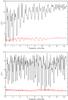 |
Fig. 1 Frequency spectra of the goodness-of-fit parameter χ2/ν of least squares sine wave fit to 1987 (top) and 1990 (bottom) MB91 V magnitude data. The upper fit spectrum of each panel shows the fit spectrum to the original data. The lower spectrum of the top and bottom panels is the fit spectrum after a sine wave with frequency 1.155 c d-1 (period 0.866 d), amplitude 11.7 mmag, and with frequency 10.80 c d-1 (period 0.0926 d), amplitude 9.2 mmag respectively, and appropriate phase, has been subtracted from the measured V magnitudes. |
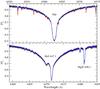 |
Fig. 2 Hα (top panel) and He i 4471 and Mg ii 4481 (bottom panel) lines observed in the 4 HARPSpol spectra, superimposed on each other. No variability is observed, in particular no possible emission variability. |
The 15 V magnitude data from the 1990 run were treated in the same way. The fit spectrum of these data is very different from that of the 1987 data. The dominant (best fit) frequency, with χ2/ν close to 1.0, is at 10.80 d-1, corresponding to a period of 0.0926 ± 0.0003 d, and the fit spectrum contains much more fine structure due to aliasing. When a sine wave of this period, amplitude 9.2 mmag, and appropriate phase is subtracted from the photometry, sine-wave fitting of the residual magnitudes yields a virtually featureless fit spectrum (bottom panel of Fig. 1). Thus, all the variation in the 1990 V data appears to be at a period of 0.0926 d. There is no hint at all of the three period aliases that dominate the 1987 data. This situation certainly raises questions as to whether the periodic variation seen in 1987 could actually be a rotation period.
Since the obvious photometric variations occurring in the two data sets are dominated by such very different frequencies, we did not carry out sine wave fitting to the two data sets combined.
4.3. Absence of emission and spectrum variations
No emission was observed in the Balmer lines of our HARPSpol spectra (see top panel of Fig. 2) contrary to what was proposed by MB91 as a consequence of the rapid rotation corresponding to their adopted rotation period.
Photometric measurements of line strength by Pedersen & Thomsen (1977) found marginal evidence for a period P = 23 d in the line strength of the He i line at 4026 Å. The line variations in this star were, however, described as being very close to the threshold of detectability, and this period has not emerged in other data.
Although we have spectra of very high resolving power and S/N, we observe no significant variability in the equivalent widths, depths, or profiles of the spectral lines of HD 96446, of the kind we would expect to find in a magnetic chemically peculiar star. Figure 2 shows the Hα, He i 4471 and Mg ii 4481 lines of the four superimposed HARPSpol spectra and indeed reveals no variation in these lines.
4.4. Radial velocity variations
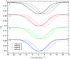 |
Fig. 3 LSD I profiles of individual subexposures obtained using the mask with all but He lines. The subexposures of the 4 polarisation measurements are shown from top to bottom. The profiles have been arbitrarily shifted by –0.1, –0.2 and –0.3 in intensity to ease the reading of the figure. The 4 subexposures of each polarisation measurements are drawn with solid, dotted, dashed, and dahsed-dotted lines in chronological order. |
When examining the LSD profiles of the four sub-exposures making up each polarisation measurement, we noticed very significant variation in the radial velocity of the mean profile from one subexposure to the next, with a pattern which suggests periodic variation with a period of the order of 0.1 d.
We therefore measured the radial velocity of each individual subexposure obtained with HARPSpol by fitting a Gaussian to the LSD I profile calculated with the mask including all metallic lines except He. The measurements are listed in Table 3. The typical uncertainty is 0.1 km s-1.
We measured substantial radial velocity variations between the individual subexposures (see Fig. 3), over a velocity range of about 6 km s-1. In principle, these variations could be the result of either binarity or pulsations. HD 96446 is a B2 star and therefore could well be a pulsating star of β Cep or SPB type, or both (a “hybrid” pulsator). As mentioned above, MB91 already detected variations with a period at 0.26 d, which they interpreted in terms of pulsations.
We performed a search for periodicity in the radial velocity measurements using our non-linear least-squares sine wave fitting programme and found a unique period at P = 0.09291 ± 0.00003 d, i.e. about 2.23 h. A sinusoidal fit of the data leads to a mean radial velocity of 3.8 km s-1 and a semi-amplitude of 4.1 km s-1. The lower portion of the spectrum of the goodness-of-fit parameter χ2/ν as a function of frequency for the original radial velocity data, and the full spectrum for the data with a sine wave of period 0.09291 d, amplitude 4.1 km s-1, and appropriate phase subtracted, are shown in Fig. 4. This period fits the radial velocity measurements very well, with a minimum χ2/ν = 1.61 (assuming a standard error of 0.1 km s-1; see Fig. 5). Note that in the prewhitened fit spectrum there is no trace of the 0.85 d period, nor indeed of any further period.
Fixing the minimum radial velocity to phase 0, we derived the ephemeris  (1)A dynamical plot of the 16 LSD I profiles, folded in phase with this ephemeris, is shown in Fig. 6. The bottom panel shows the residuals obtained from a profile calculated by shifting the 16 profiles to a radial velocity equal to 0 and averaging these 16 recentred profiles. The average profile obtained this way is shown with a dashed red line in the top panel of Fig. 6.
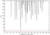 |
Fig. 4 Frequency spectra of the goodness-of-fit parameter χ2/ν of least squares sine wave fit to our HARPSpol subexposure radial velocity data. The upper fit spectrum shows the fit spectrum to the measured data from Table 3. The lower spectrum is the fit spectrum after a sine wave with period 0.09291 d, amplitude 4.1 km s-1, and appropriate phase has been subtracted from the measured radial velocities. |
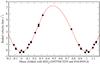 |
Fig. 5 Radial velocity measurements folded in phase with the period P = 0.0929 d and HJD0 = 2 455 704.5255. The solid red line shows a sinusoidal fit to the data. |
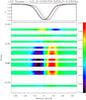 |
Fig. 6 Top panel: LSD I profiles (black solid lines) of individual subexposures obtained using the mask with all but He lines and the average profile (dashed red line, see text). Bottom: dynamical plot of the residuals of the profiles relative to the mean profile, folded in phase with P = 0.0929 d. The vertical dashed lines indicate ± 4.112 km s-1 centred on 3.8325 km s-1 and correspond to the excursion domain of the centre of the line. |
The P = 0.0929 d period corresponds, within uncertainties, to the period detected in the MB91 photometry from 1990. This period is typical of β Cep-type p-mode pulsations (Aerts et al. 2010). Consequently, we interpret both the radial velocity variations and the photometric variations found in the 1990 V photometry from MB91 as caused by the presence of a pressure mode of β Cep-type pulsations. The main mode of β Cep stars is often a radial mode. Radial modes are at the origin of stronger radial velocity shifts than non-radial modes. Therefore, the pulsation mode detected here may be radial. Note, however, that pulsation modes, especially radial ones, usually produce not only a velocity shift but also an asymetric distortion of the profiles. This distortion is not clearly observed here, probably because vsini is small while the Zeeman line broadening is large. However, as we will see below, we find indication of this distortion when calculating LSD V and N profiles.
To summarise, we find clear evidence in the available photometry and our own radial velocity measurements of variability with two periods. The period P = 0.0929 d which is found in our HARPSpol subexposure velocities, and in the 1990 (but not the 1987) V photometry of MB91, is probably a β Cep pulsation period. The second period, which might be near 0.47, 0.87, or 6 d, but is most probably about 0.87 d, has been interpreted as the rotation period of HD 96446 (MB91). However, the absence of this period in the 1990 V photometry of MB91 makes this identification uncertain. This period may instead be a symptom of SPB star g-mode pulsation, which typically occurs with one or more periods of the order of one or several days. Thus HD 96446 may be a “hybrid” B pulsator. In this case however, the detection of the g-mode but not the p-mode in the 1987 data would suggest that the amplitude of the respective modes changes significantly with time. We will look for further evidence about the nature of the 0.87 d variation below.
5. HARPSpol magnetic field measurements
5.1. Effects of radial velocity variations on the LSD profiles
The HARPSpol observations of HD 96446 were carried out using the beam exchange technique, widely used in high-resolution spectropolarimetry (Donati et al. 1997; Bagnulo et al. 2009). As described above, four sub-exposures with different orientation of the quarter-wave retarder plate were combined using the “ratio method” to produce the Stokes V spectrum and a null N spectrum, which is used to diagnose possible spurious polarisation. This procedure assumes that there is no intrinsic change of the stellar spectra for the entire duration of observations. Examination of the Stokes I of individual sub-exposures of HD 96446 showed that this assumption is not satisfied for this star as there are definite radial velocity variations with P = 2.23 h. A consequence of these velocity shifts could be spurious signatures or distorsion of Stokes V and N spectra. It is therefore important to assess how much the radial velocity shifts affect the observed Stokes V and N signatures, and in particular if they could explain the weak variations observed in the Stokes V profiles (see top curves in left panel of Fig. 8).
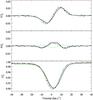 |
Fig. 7 Simulated Stokes V (top), N (middle) and I (bottom) spectra assuming a −1 kG field and the radial velocity shifts measured in Sect. 4.4. |
Using LSD Stokes I profiles extracted from individual sub-exposures, we have quantitatively assessed the impact of velocity shifts on both the N and V signatures. Assuming a line of sight field of −1 kG and using the weak field approximation, we have computed synthetic LSD Stokes V profiles from the derivative of the corresponding I spectra, created the right- and left-hand polarised beams (I ± V) and used the resulting spectra as an input for the same demodulation procedure as was applied to observations. The resulting Stokes I, V and N spectra are illustrated in Fig. 7.
We found that the relative amplitude and shape of the N signatures can be attributed to velocity shifts. In particular, a different shape of the N profile for the third observation (see middle curves in left panel of Fig. 8) is explained by a different direction of the velocity change. Consequently, there is no doubt that the N signatures are directly linked to the line profile variations and in particular the radial velocity shifts.
At the same time, the distortion of the synthetic Stokes V is weak compared to the changes observed in the HARPSpol profiles and it does not visibly affect the longitudinal field measurements: the mean field from four sub-exposures always deviates by less than 1% from the value derived from the demodulated Stokes V signal. Consequently, the effect of the radial velocity shifts on the Stokes V profiles is negligible. The Stokes V signatures are due to the presence of a magnetic field and not to the radial velocity shifts, and the velocity shifts cannot account for the weak variations observed in the Stokes V profiles.
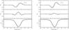 |
Fig. 8 LSD V (top), N (middle), and I (bottom) profiles of HD 96446 calculated using all photospheric but H and He lines, without (left) or with (right) correction of the radial velocity shifts. Full black line: 23/05, red-dashed line: 24/05 3:30, green dot-dashed line: 24/05 23:14, blue dot-dot-dashed line: 27/05. The mean error bars are plotted in the top box with the respective colour and in chronological order. |
Nevertheless, we corrected the individual exposures from the radial velocity shifts and recalculated the LSD profiles from these corrected data (see Sect. 2). The right panel of Fig. 8 shows that indeed this correction significantly reduced the N signatures, although some signal remains due to the line profile distortions that are not corrected for. The weak variability in the Stokes V signatures does not disappear after the correction for radial velocity shifts, which confirm that these variations are related to the magnetic field itself.
5.2. ⟨ Bz ⟩ measurements and Stokes profiles
Using the Stokes I and V profiles calculated with the LSD submasks described above, we measured the longitudinal magnetic fields of each observation, as described in Alecian et al. (2009). We performed this calculation with and without correcting for the radial velocity shifts in the individual subexposures. The results we obtained are compatible, within the error bars, whether or not we corrected for the radial velocity shifts. In the remaining of the paper, we use the corrected LSD profiles.
For this calculation we integrated over a velocity range of ± 20 km s-1 for masks that included all lines except He lines, as well as for the masks with only O or C lines, while we integrated over ± 100 km s-1 for the He line mask. We also calculated the longitudinal magnetic field in the Hα line. In this case we integrated over a velocity range of ± 60 km s-1, which is the range that shows Stokes V signal. The values are reported in Table 4 for each submask. The full range of the I profile of the Hα line covers ± 470 km s-1.
The values we obtained from the mask with all but He lines or with He lines only were very similar to each other, despite the difference in the I profiles and width of the integration range used in the LSD. They were also similar to those obtained by Mathys (1991). Longitudinal field values obtained from O or C lines only were different by ~100 G but were however compatible with those obtained from using only He lines, within the error bars. From the core of Hα we obtained field values about 500 G lower than for other lines. In the literature (MB91, Mathys 1991) a discrepancy of ~700 G had already been noticed between field measurements made using the wings of Hβ and metallic lines. However, H lines are more difficult to analyze because of their broad wings and these new longitudinal field values may therefore be influenced by the I profile. Integrating over a velocity range that includes the full wings provides field values that are compatible with the ones found using LSD for other lines in the HARPSpol spectra. However, the longitudinal field calculated using this full range led to more variable values for the four measurements and was dominated by noise.
In our four polarised spectra obtained over four nights, we detected clear Zeeman signatures in many individual spectral lines in addition to the signatures observed in the LSD V profiles (top curves of Fig. 8). Using LSD profiles, however, provides more accurate measurements of the longitudinal magnetic fields. Small but significant variations in the V spectrum, as well as in the longitudinal magnetic field values, were detected during the run while the four observations were obtained at three different rotational phases (see Table 1). Assuming Prot = 0.85 d (MB91), observations #2 and #3 were indeed taken at about the same rotation phase, however the V profiles of #1 and #2 ressemble each other more.
The lack of strong variation in the Stokes V profiles indicates that only one magnetic pole is visible over the rotation period. Together with a low vsini, it suggests a low inclination angle i, as predicted by Shore & Brown (1990) from UV wind lines and determined spectroscopically (i ≤ 4°) by Zboril & North (1999).
Using i = 3° and β = 65° (see Sect. 1), we found that our ⟨ Bz ⟩ measurements are compatible with a dipole field with Bpol ~ 9000 G.
6. Spectrum modelling
For many kinds of early-type peculiar stars, the physical situation in the atmosphere may be rather complex. If a magnetic field is present, it has some unknown distribution of field strength and direction over the stellar surface. Various elements in the atmosphere may be distributed non-uniformly, in the form of patches, and may also be non-uniform in the local vertical direction (stratification). Pulsation may also be present. All of these complications modify the spectral lines produced by the atmosphere, and to extract useful information about stellar parameters these phenomena are either treated in a rather approximate way, or require detailed modelling with appropriate inversion codes.
Hotter stars, with effective temperatures above about 15 000 K, have the additional complication that many atomic levels have populations not accurately predicted by the assumption of LTE (for more discussion see Lanz & Hubeny 2007). These effects are modelled by specialised non-LTE radiative transfer codes, which in general do not have descriptions of any of the other phenomena mentioned above built into them. Thus we have a dilemma – to use spectrum synthesis codes with the capability of modelling the complications specific to upper main sequence magnetic and chemically peculiar stars, or codes designed to deal with non-LTE level populations. Neither solution is very satisfactory.
Recently, Przybilla et al. (2011) have demonstrated that there is a viable compromise solution to this problem. They have carefully compared the output of their non-LTE line synthesis method, based on ATLAS9 LTE model atmospheres and the non-LTE codes DETAIL and SURFACE, with high-S/N, high-resolution spectra of a number of early B stars for which they have determined very accurate fundamental parameters, and have established which observed lines are well reproduced by their own synthetic spectra. Then they have compared the output of their code with both fully LTE calculations using ATLAS/SYNTHE, and non-LTE synthesis using TLUSTY/SYNSPEC. They have shown that for many lines of some important ions, and for some lines of most ions studied, the results of LTE synthesis yield correct line profiles and deduced abundances up to Teff ≈ 22 000 K. Thus it appears that we can use an LTE line synthesis code to model spectral lines in an early B magnetic star, such as HD 96446, provided we can identify spectral lines for which LTE computations give largely correct results. In addition, the spectral lines of HD 96446 are quite sharp, which should provide strong constraints on certain parameters.
To study the line profiles of HD 96446, we use the programme ZEEMAN (Landstreet 1988), which computes synthetic spectra in LTE for specified values of Teff and log g. The computed spectrum is compared to the observed one, and parameters can be iteratively adjusted to find abundances log (NX/NH) together with the best fit radial velocity Vrad, rotational velocity vsini and microturbulence parameter ξt. For a magnetic star it is usually assumed that ξt = 0, but line broadening is provided by Zeeman splitting. ZEEMAN can correctly compute the polarised spectrum of a star permeated by a specified magnetic field: the four equations of radiative transfer for the four Stokes components are solved simultaneously, taking into account the polarisation properties of the various component of the spectral lines, which are split and polarised by the Zeeman effect.
6.1. Mean field modulus and v sin i
A first reconnaissance was carried out by modelling the three fairly strong lines of Si iii at 4552, 4567 and 4574 Å in the HARPSpol I spectrum #3 of HD 96446. These lines are subject to rather large non-LTE corrections (Becker & Butler 1990a,b), but although the abundance of Si derived from LTE spectrum synthesis of the lines is seriously in error, line shape parameters are trustworthy. Assuming at first that the magnetic field effects on the line shapes are negligible, we find that the best joint fits to the three Si iii lines occur for ξt = 5 ± 1 km s-1 and vsini = 5 ± 2 km s-1. Thus the projected rotational velocity is very low indeed.
However, the magnetic field of this star is sufficiently strong that it does affect the line shapes, and so the vsini value needs to be found from a synthesis including the effect of the field. From the discussion above of magnetic measurements of the star, it seems very likely that ⟨ Bz ⟩ values of at least 1500 G occur at times. From studies of other magnetic stars, it is found that the mean field modulus ⟨ |B| ⟩ must be of order three or more times larger than the largest ⟨ Bz ⟩ value (Landstreet & Mathys 2000), so the typical field strength in the stellar atmosphere is expected to be of order 5000 G. This is large enough to produce detectable line splitting in the I spectrum, and in fact when the same three strong lines of Si iii were modelled with a field of this order, it was found that (1) the various line shapes are better predicted with broadening produced by a magnetic field than with vsini or microturbulent velocity broadening; and (2) that the maximum value of vsini decreased to or below the value of 5 km s-1 found with non-magnetic spectrum synthesis.
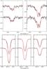 |
Fig. 9 Upper panel: LTE fit of strongly Zeeman split Fe iii lines at 5063 and 5074 Å with ⟨ |B| ⟩ = 4800 G and vsini = 3 km s-1. The fits are shown to the two spectra (#3 and #4) that clearly reveal splitting of the 5074 Å line. Lower panel: comparison of LTE fits to Si iii 4552, 4567 and 4574 lines in spectrum #3 with ξt = 5, vsini = 6 km s-1 and no magnetic field (upper curves), to LTE fits (lower curves) with the magnetic model of the upper panel. |
To obtain a more precise measurement of ⟨ |B| ⟩ , a search was made in the stellar spectrum for lines of useful depth with particularly large Zeeman splitting. The Fe iii lines at 5063 and 5074 Å, which have a Landé factor of 2.5 and 2, respectively, i.e. which are strongly split by the magnetic field, were selected for closer study. In the I spectra having the highest S/N, the 5074 Å line is clearly split by the field into a doublet, and the 5063 Å line has a rather square, broad profile, also due to Zeeman splitting. We fitted LTE models to these lines and found a best fit with ⟨ |B| ⟩ = 4800 G and vsini = 3 ± 2 km s-1. Fitting again the Si iii line triplet at 4552, 4567 and 4574 Å showed that this field strength is consistent with the variation of the line profiles (Fig. 9). Values of vsini ≥ 6 km s-1 can therefore definitely be excluded.
The magnetic line splitting was detected clearly in HARPSpol spectra #3 and #4. The other two spectra do not have high enough S/Ns for the splitting to be clearly observed. For the two spectra in which splitting is detected, the same value of ⟨ |B| ⟩ was found.
6.2. Magnetic field structure and inclination i
With now more than 20 measurements of the magnetic field strength ⟨ Bz ⟩ available, two measurements of ⟨ |B| ⟩ , an upper limit to vsini, and a provisional rotation period of 0.85 d found by photometry, we can consider what constraints can be put on the magnetic field structure of HD 96446.
Several important problems are presented by this rather large amount of data. (1) The three available sets of measurements of ⟨ Bz ⟩ do not agree among themselves very well. There seems to be an overall uncertainty in the scale of the field of almost a factor of two, and also some significant uncertainty about how variable it is. (2) Although a very tight constraint is available on vsini, it appears that a still smaller value than the safe upper limit of 6 km s-1 may apply. This would strongly constrain possible models (as we will see below). (3) It is very uncertain that the 0.85 d period is actually the rotation period. Furthermore, we will see below that such a short period creates real difficulties for the magnetic field model.
We first assume that the rotation period is actually 0.85 d, and that the value of vsini is about 3 km s-1. veq is then 266 ± 120 km s-1 (where the 1σ error bar follows from the error on the radius), i.e it has a minimum value of 146 km s-1. Therefore the value of i is no larger than about 1.2°. Even if vsini is as large as 6 km s-1, the maximum allowed value of i is only about 2.3°, and it is very likely closer to 1°. We now consider a field model of a simple magnetic dipole of polar field strength Bpol, inclined by an angle β to the rotation axis. The importance of such a simple model is that most of the contribution to the observed ⟨ Bz ⟩ comes from this component of the actual, more complex, field; higher order field moments are very inefficient at producing globally coherent longitudinal field (Landstreet 1988). In this model possible variations of the longitudinal field are due to the line of sight rotating around the stellar rotation axis, and viewing the global field from different directions.
We may obtain a first estimate of the global field using a simple relationship found by Preston (1967):  (2)where r is the ratio of the smaller extremum value of ⟨ Bz ⟩ (of either sign) to the larger extremum value; r can take any value from + 1 to −1 for different stars. The field values are usually taken from the variation of ⟨ Bz ⟩ with rotational phase, but if this is not known, they may be estimated from the observed range of values. MB91 have phased the magnetic data with their 0.85 d period; the resulting variation suggests that r ≈ 0.63 for the Balmer line magnetograph field measurements, while rescaling the CASPEC data from this curve to the original values gives r ≈ 0.42. From the smaller set of ⟨ Bz ⟩ measurements from HARPSpol, which may not cover the full range of field strengths, we estimate r ≈ 0.77. From Eq. (2), it is clear that a very small value of i, as we have for the period P = 0.85 d, leads to a large value of β. For the three ⟨ Bz ⟩ data sets, assuming i is 2.3°, its upper limit, we find β values of respectively 80°, 84°, and 73° (Balmer line, CASPEC, and HARPSpol). That is, the dipolar component of the field distribution must be observed from near the magnetic equator in order for the field variations observed to be possible with an excursion of the line of sight closer to and farther from the negative magnetic pole by less than 5°.
But if the magnetic field is observed along a line of sight that is almost perpendicular to the field axis, the polar field must be very large for the component along the line of sight to be as large as 1−2 kG. Using the results from Landstreet (1988), we estimate roughly that the polar field strength of the required dipole component is of order 30 kG if the Balmer line or CASPEC field strengths are most representative of the stellar field, or at least about 10 kG on the basis of the less complete set of HARPSpol field measurements.
We next consider whether these large deduced polar field values are consistent with the measured values of ⟨ |B| ⟩ , about 4800 G. Landstreet (1988) has shown that for simple field models, the value of ⟨ |B| ⟩ is generally at least about 0.6 times as large as the polar field. This completely rules out the field model we are considering on the basis of the Balmer line and CASPEC magnetic measurements; the predicted value of ⟨ |B| ⟩ is about three times larger than the observed value. If the older magnetic measurements underestimate r and/or overestimate the global field strength, and the four HARPSpol measurements are more representative, then this model is marginally possible, by tuning all the parameters to their limiting values. Thus the very small value of i implied by the assumption that 0.85 d is the rotation period makes it very difficult to find even a very simple, fully consistent model of the magnetic field.
On balance, it appears that the assumption that the period of rotation is the 0.85 d period detected in the photometry may well be incorrect. This is already suggested by MB91 as well as by our own analysis (see Sect. 4.2). This suspicion about the very short period (and very small i) is reinforced by the fact that the range in V magnitude is about 0.02 mag, with a displacement on the observed stellar hemisphere of at most 4.5°. If this same star were observed from a different direction, such that i were, say, 40 or 50°, we would expect a variation in V magnitude at least roughly 10 times larger, which would suggest a variation in V almost an order of magnitude larger than is usually seen in magnetic Ap-Bp stars. Again this seems unlikely.
Therefore we consider the possibility that the rotation period is several days (as suggested by measurements of ⟨ Bz ⟩ obtained over three consecutive nights in all three types of magnetic data) rather than 0.85 d. In this case the value of i is not strongly constrained by the ratio of vsini to veq; i could be as large as perhaps 30°. If this were the case, the constraints on the magnetic field model become much less severe. The observed variation in ⟨ Bz ⟩ can be obtained from a line of sight that passes much closer to the magnetic pole, so the required polar field strength is smaller, and can easily be made consistent with the observed values of ⟨ |B| ⟩ .
Field models that satisfy these relaxed constraints can be found by using the tools described by Landstreet & Mathys (2000). It is found that there are reasonable models consistent with any one of the three ⟨ Bz ⟩ datasets. Each of the three models involve (dipole) polar field strengths of several kG (5000 to 10 000 G), values of β in the range of 35 to 60°, and values of i between 4 and 15°. Since, with the period unknown and the apparent inconsistencies between ⟨ Bz ⟩ data sets, we do not know enough to specify which (if any) of these models is correct, it is perhaps best to adopt a very schematic model for the long-period case. We adopt i = 10°, β = 45°, and Bpol = 6500 G as reasonably representative parameter values to use in the rest of the paper.
The parameters determined here are summarised in the bottom part of Table 2.
6.3. Abundances
Chemical abundances in peculiar stars provide very important constraints on physical processes that occur in the upper envelopes of such stars. These abundances reflect the competing actions of atomic diffusion under the influences of gravity and radiative levitation, of mixing processes such as convection and meridional circulation, and of mass loss, some or all of which may be modified by the presence of a magnetic field. It is therefore quite valuable to determine the abundances of elements in the stellar atmosphere.
To enable us to identify spectral lines for which LTE computations give correct abundances, we have adopted a simple method. We have available an ESPaDOnS spectrum of the hot non-magnetic star α Pyx = HD 74575, for which the fundamental parameters and the abundances of common elements have been determined with extremely high precision by Przybilla et al. (2008), and whose fundamental parameters are only slightly different from those of HD 96446. We have carried out spectrum synthesis of α Pyx with the parameters and abundances found by Przybilla et al., and identified spectral lines whose strengths are correctly computed using LTE. Then we use our magnetic LTE code ZEEMAN to synthesise various spectral regions of HD 96446, adjusting the adopted abundances to fit those lines identified from the α Pyx study as safe to use in LTE. In general, to avoid problems connected with the different behaviour of lines broadened by microturbulence compared to lines broadened by a magnetic field, we have tried to use mostly rather weak lines, with equivalent widths Wλ of less than about 50 mÅ.
Using this technique, we have been able to obtain reasonably reliable hemispheric average abundances for 10 chemical elements in the atmosphere of HD 96446, as listed in Table 5. The uncertainties are estimated from discrepancies from one region to another, or from estimates of the effect of using only one or two lines.
For He, there are several lines of He i, and one of He ii, that are well fit in α Pyx with LTE computations at solar abundance. Furthermore, Przybilla et al. (2011) have shown that the lines used by us are well modelled around the temperature of HD 96446 by LTE synthesis. The lines listed in Table 5 were fit by adjusting the abundance of He, and a general best fit is found with more than four times the solar abundance of He. The star is definitely He-rich. However, all the He i line profiles fit in HD 96446 are poorly matched by the computed profiles, in all cases in the sense that the computed cores are too strong, while the computed wings are not deep enough (Fig. 10). The simplest interpretation of this result is that He is somewhat stratified in HD 96446, with a higher He abundance near continuum optical depth one, where the strong damping wings are formed, compared to the abundance at small continuum optical depth.
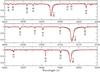 |
Fig. 10 Three spectral windows in HD 96446, each containing a single He i line. The observed spectrum (#3) is shown in black, the LTE fits in red. |
A visible peculiarity of the He i line at 4713 Å is that it shows a strong asymmetry: the core has a bulge on the long-wavelength side, and the wing on the same side of the line is broader and deeper than that on the short-wavelength side. This is due to the fact that this line is a triplet, with a weaker component 0.2 Å longward of the main component, producing a clearly visible asymmetry in the computed profile because the star has such a tiny projected rotation velocity. The similarly strong singlet line at 5047 Å shows no strong asymmetry. However, the singlet line at 4437 Å has a more puzzling profile. This line is strongly asymmetric, with a depressed long-wavelength wing. A similar asymmetry is seen in the magnetic Herbig AeBe star HD 200775 (Alecian et al. 2008), but there it seems to be a consequence of binarity. There is no known blending line here. The most plausible explanation for the asymmetry in this line is that it is the result of the presence of a blend with a 3He line, which is visible in a few stars of exceptionally low vsini (Bohlender 2005, see also Bohlender et al., in prep.). Several He i lines are illustrated in Fig. 10.
Most of the lines of C that are present in the spectrum are lines of C ii. Almost all of them are considerably weaker in α Pyx than in the computed LTE spectrum, and cannot be reliably used for abundance analysis. Przybilla et al. (2011) have also shown that most lines of C ii are unsuitable for LTE abundance analysis. However, according to Przybilla et al. (2011) and our own experiments, the triplet of C iii lines at 4650 Å seems reliable, as does multiplet (16) of C ii, and these lines have been used to obtain the abundance of C.
Many lines of N ii and O ii are present in the spectrum. In α Pyx, the LTE synthesis tends to agree with the weaker observed lines but to predict lines that are too strong for stronger observed lines. Thus weaker lines were used for abundance analysis. However, in HD 96446 the LTE abundances that correctly reproduce the weak lines used mostly give good agreement with the stronger lines as well. These two elements tend to be well reproduced by LTE line synthesis in this star, consistent with the conclusions of Przybilla et al. (2011).
The abundance of Mg has been found from a single strong line, at 4481 Å, which is not in the dominant ionisation stage. Nevertheless, synthesis of this line for α Pyx suggests that the line gives usefully accurate results.
Si has a number of obvious lines in the spectrum of HD 96446. However, judging from the synthesis of the spectrum of α Pyx, most of these lines are strongly out of LTE. LTE abundances deduced from lines of Si ii are at least a factor of 10 lower than those deduced from lines of Si iii. The calculations of Becker & Butler (1990a,b) certainly suggest that this is the case, but even these NLTE line strength computations do not represent well the full extent of departure from LTE, and do not yield concordant abundances of Si ii and Si iii for α Pyx. We have relied on one line of Si iii at 4683.02 Å, for which LTE line strength computations are consistent with the essentially solar Si abundance claimed by Przybilla et al. (2008), and one line of Si iv at 4654.31 Å. LTE computations of line strengths of other Si lines with the adopted abundance of Si for HD 96446 show discrepancies compared to the observed lines that are quite large, but similar to those found from solar abundance LTE computations for α Pyx.
A few lines of S ii that are well fit in α Pyx suggest that the abundance of this element is almost one dex below the solar value.
Several weak lines of Ar ii are well fit in α Pyx with solar abundance in LTE, and well fit in HD 96446 with an underabundance of about a factor of two.
Fe iii is represented by weak lines of multiplet (4), around 4400 Å, and multiplet (5), around 5100 Å. Most of these are well fit in α Pyx with solar abundance, and in HD 96446 with an iron abundance about two times lower. Two of the lines of multiplet (5) have unusually large Landé factors, and are the lines used to estimate the value of ⟨ |B| ⟩ above.
The general quality of the LTE fits is shown in three spectral segments in Fig. 10. Overall, although the synthetic spectrum is computed in LTE, the fit to most lines is quite reasonable. One glaring exception is the Si ii 5041 Å line, which illustrates the large discrepancies found between LTE line computations and some of the observed lines, particularly for Si.
The important conclusion that emerges from Table 5 is the following: although the spectrum of HD 96446 does not appear on casual inspection to be particularly unusual for a B2 main sequence star, it seems to reveal substantial chemical peculiarities in addition to the characteristic of having a He-rich atmosphere. In fact, every other element for which we are able to obtain an abundance seems to be underabundant with respect to the solar abundances, by a factor of typically 2.5 to 5. Thus, any model that is invoked to explain the overabundance of He in the atmosphere should be able to explain the widespread underabundances of most other light elements. Either these elements are sinking down below the stellar atmosphere, or they are being ejected upwards more rapidly than they are being replenished from below.
6.4. Non-LTE sanity check
NLTE synthetic spectra were calculated using the TLUSTY BSTAR2006 grid of model atmospheres (Lanz & Hubeny 2007) and the SYNSPEC code (version 48; Hubeny 1988; Hubeny & Lanz 1992). Contrary to the LTE models, the NLTE models do not include magnetic fields. They are calculated here only to confirm that the parameters and abundances determined from LTE modelling are not influenced too much by NLTE effects.
We calculated synthetic spectra with Teff = 21 000 K, log g = 4.0 with both solar abundances and with the abundances determined from the LTE modelling above (see Fig. 11). To be consistent with our LTE models, we use the solar abundances of Asplund et al. (2009) rather than those of Grevesse & Sauval (1998) used by default in the BSTAR2006 grid. Overall, and especially for strong lines, the abundances determined from the LTE modelling fit the observed spectrum better than the solar abundances, although some weak lines are less well fitted. Some of these discrepancies are probably due to blends or possibly to the presence of the magnetic field. This confirms that the parameters and abundances determined from LTE modelling are adequate.
Figure 12 shows the NLTE models for the Si iii triplet at 4552, 4567 and 4575 Å with the two sets of abundances. As expected, neither the solar abundances nor those determined with the LTE modelling fit the observed spectra well. The tests presented in Przybilla et al. (2011) show that LTE models can be superior to NLTE models, even for hot stars, when the chosen atomic models used for the NLTE computations are too simplified. In particular, Przybilla et al. (2011) suggested that the Si atomic model used in TLUSTY/SYNSPEC is too schematic. See also the discussion about these lines in Sect. 6.3.
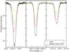 |
Fig. 12 NLTE models with solar (red line) and LTE abundances (green line) of the Si iii triplet. |
For HD 96446, we conclude that our LTE and NLTE modelling are consistent, and that the precision on the stellar parameters and abundances determined from the LTE modelling is sufficient for the goal of the present paper.
7. Magnetospheres
7.1. Magnetic confinement
The competition between the magnetic field and stellar wind is characterised by the magnetic confinement parameter, η∗, defined by ud-Doula & Owocki (2002), which depends on the stellar equatorial magnetic field strength, radius, and wind momentum. When η∗ > 1, wind material can be channeled and confined into a circumstellar magnetosphere.
For a dipolar field, above the Alfvén radius  , the wind dominates and stretches open the magnetic field lines. Below RA, the wind material coming from both magnetic hemispheres is trapped in closed magnetic loops. If stellar rotation is weak, the material is pulled back onto the stellar surface by gravity.
However, for a star with rotation period Prot and surface orbital period Porb ≡ 2πR/vK (where  is the Keplerian orbital speed for the assumed stellar mass M and equatorial radius R), material trapped at or above the Kepler co-rotation radius RK ≡ (Porb/Prot)2/3 can be centrifugally supported against gravitational infall. In cases with RA > RK, this rotationally supported, magnetically confined material accumulates to form a centrifugal magnetosphere (CM). But when RK > RA > R, i.e. strong magnetic confinement but slow rotation, the transient suspension of material in closed loops leads to a dynamical magnetosphere (DM). See ud-Doula et al. (2008), Petit et al. (2012) and Sundqvist et al. (2012) for more details.
HD 96446 is very similar in mass and temperature to σ Ori E, the prototype for the CM model. Its wind was detected in UV lines with a terminal velocity close to v∞ = 1000 km s-1. From our magnetic measurement we estimated the polar field strength of HD 96446 to be ~9000 G, while the spectrum modelling led typically to ~6500 G. With a stellar radius R = 4.45 R⊙ and assuming a mass-loss rate similar to σ Ori E (~10-9 M⊙ yr-1), the magnetic confinement parameter η∗ is of order 105, meaning that matter should be strongly confined in the magnetosphere. Reducing η∗ to unity would require Bpol < 16 G, a value completely excluded by our observations. Even assuming a much stronger mass loss than the one of σ Ori E, the required Bpol would be much lower than the observed one to reach η∗ < 1 (see the upper section of Table 6).
7.2. Centrifugally supported magnetosphere
The MB91 rotation period of 0.85 d is a plausible factor (~2.2) longer than the surface orbital period of Porb = 0.38 d, and moreover seems to fit well with some of the historical magnetic data. For such a period, one obtains a Kepler radius RK ≈ 1.6R that is substantially within the Alfvén radius, RA ≈ 20.1−23.6R. This suggests that HD 96446 is rotating fast enough to have a stable CM.
However, no sign of the presence of confined material was detected in our data, for example through Hα emission. In addition, there is no detection of X-ray emission: measurements by Grillo et al. (1992) give an upper limit on the X-ray luminosity an order of magnitude lower than observed from σ Ori E.
One explanation for the lack of confined material in spite of the large η∗ could be that the wind is not dense enough to form emitting clouds, or that it does not cool to a temperature at which Hα is strongly emitted. However, given the similarity in spectral type to σ Ori E, the mass loss rate, and the cooling rate, should be quite similar. Given also the similarity in RA and RK, the characteristic magnetospheric confinement time tconf should be similar as well (of the order of a few months), implying then a comparable magnetospheric mass Ṁtconf (where Ṁ is the mass loss rate) and emission measure  , and consequently a similar level of Hα emission.
Assuming that Prot = 0.85 d, the fact that HD 96446 shows no such emission would thus represent a serious challenge to the CM model that had proved so successful for modelling σ Ori E.
7.3. Constraints on possible longer rotation period
As one potential solution to the puzzling lack of magnetospheric emission, let us consider now whether the actual rotation period could be substantially longer than the MB91 inferred value of 0.85 d. In the present paper, we have already questioned the correctness of this rotation period.
First, for the vsini = 3 km s-1, as determined in Sect. 6.1, i has to be lower than 30° for any rotation period considered in this article (see Sect. 6.2). Because we do not expect much visible rotational modulation (nor ⟨ Bz ⟩ modulation) when i is small, the detection of P = 0.85 d in photometric data of MB91 might instead be attributed to pulsations. Indeed Mathys (1994) already pointed out that, when assuming Prot = 0.85 d, the oblique rotator model is not satisfactory.
We showed above that the MB91 photometric data can also be phased relatively well with Prot = 5.73 d. This gives a Kepler radius RK ≈ 5.5R with the adopted M that, while still much below the Alfvén radius RA ≈ 20.1−23.6R, now implies that the accumulated high density material is distributed over a much larger volume. Still, only a much stronger (probably unrealistic) mass loss rate would make it possible to decrease RA to RK (see the middle part of Table 6).
However, even under the conservative assumption that the total confined mass Ṁtconf is not reduced by the increased RK (e.g. by a smaller confinement time by the weaker field, or the reduced solid angle of stellar wind feeding regions at or above RK), the overall emission measure should be reduced proportionally to the inverse of the volume ( ). Compared to the previous assumption of Prot = 0.85 d and thus RK = 1.6R, adopting instead a rotation of 5.73 d with RK = 5.5R thus implies a substantial reduction (1.6/5.5)3 ≈ 0.02 in the emission measure. In this case, the resulting net Hα emission may indeed not be detectable, thus explaining the lack of observed emission for HD 96446. Theoretical work about these scaling issues is discussed in more detail in an upcoming paper by Petit et al. (in prep.); see also Townsend (2008).
Using the fundamental parameters of the star derived above, a rotation period of several tens of days would even be possible. The last part of Table 6 shows that any period up to Prot = 39.8 or 50.7 d (for Bpol = 6500 or 9000 G, respectively) would lead to RA > RK, i.e. a CM. This implies i < 32 or 42.5°, respectively.
In the case of a large angle i, rotational modulation of the magnetic data should lead to Stokes V profiles that are varying significantly in shape. The Stokes V profiles observed in the historical magnetic data as well as in our HARPSpol data are always similar and correspond to the negative pole seen pole-on. This behaviour does not fit with a large i angle. Following Sect. 6.2 we must keep i < 30°, i.e. the rotation period should remain below 19.3 days (see last line of Table 6).
Therefore we conclude that Prot must be long enough (several days) to explain the lack of Hα emission in a CM, but not too long (below ~20 days) to explain the small but non-zero Stokes V variation.
7.4. Dynamical magnetosphere
Trapped material below RK lacks sufficient centrifugal support and so falls back onto the star on a dynamical (free fall) timescale, typically about a day, much less than the few-hundred-day confinement inferred for the CM of σ Ori E. Even this transient suspension still leads to a relative overdense region around the magnetic equator, representing then a DM. When RK > RA, i.e. for HD 96446 when Prot > 40−50 d and consequently i > 32−42.5°, only a DM can exist (at R < r < RA). However, when RK < RA, a DM can still exist at R < r < RK and, if η∗ > 1, coexist with a CM (at RK < r < RA).
As mentioned above, the Stokes V variations do not fit with a large angle i, i.e. with the very long rotation period required for a pure DM at R < r < RA.
For stars with a sufficiently high mass-loss rate to accumulate a suitably large magnetospheric mass Ṁtconf in the modest 1-d confinement time, there can still be substantial Hα emission, e.g. as shown by Sundqvist et al. (2012) for the slowly rotating O star HD 191612. However, in a B-type star like HD 96446, the relatively low mass-loss rate means that any dynamical infall regions do not have sufficient mass or emission measure to produce observable Hα emission. Therefore a DM could indeed exist at R < r < RK < RA in HD 96446, without producing Hα emission.
8. Conclusion
In our HARPSpol observations of HD 96446, we found clear direct magnetic signatures in the Stokes V profiles of HD 96446, and inferred slightly varying values of the longitudinal magnetic field, typical of an oblique dipole rotator observed at low stellar inclination. We also detected radial velocity variations with a period P = 0.0929 d, which we attribute to β Cep-type p-mode pulsations. Moreover, we re-determined the stellar parameters of HD 96446 and determined its chemical abundances: HD 96446 appears strongly enriched in He, similarly to σ Ori E, and depleted in all other studied elements.
Using our results for the magnetic field and the properties of the wind, we calculated that the confinement parameter is much higher than the value at which material is confined in a magnetosphere at the stellar magnetic equator. However, HD 96446 does not present signatures of the presence of such confined material; in particular, it does not show Hα emission or X-ray emission. Therefore we concluded that, even though HD 96446 is very similar to the archetypal CM star σ Ori E, its magnetosphere is different and does not produce emission.
The most likely explanation is that the rotation period is longer (between a few and 20 days) than the one proposed by MB91, i.e. long enough to shift the Kepler radius sufficiently outward to dilute the volume emission measure from a CM but short enough to keep the Stokes V variation low. In addition, a DM could be present closer to the star, without producing emission.
Since doubts have been cast on the available value of the rotation period, intensive monitoring of HD 96446 with high-resolution spectropolarimetry over a few months is necessary to determine its exact rotation period and confirm the diluted CM scenario.
Another explanation would be to invoke a leakage mechanism (see ud-Doula et al. 2008, 2009). Such models of magnetospheres including complex leakage do not exist yet but will be developed and tested within the MiMeS project.
Acknowledgments
We wish to thank the Programme National de Physique Stellaire (PNPS) for their support to MiMeS. We also thank Rich Townsend for useful discussions. J.D.L. acknowledges financial support from the Natural Sciences and Engineering Research Council of Canada. O.K. is a Royal Swedish Academy of Sciences Research Fellow, supported by grants from Knut and Alice Wallenberg Foundation and Swedish Research Council. This research has made use of the SIMBAD database operated at CDS, Strasbourg (France), and of NASA’s Astrophysics Data System (ADS).
References
- Aerts, C., Christensen-Dalsgaard, J., & Kurtz, D. W. 2010, Asteroseismology (Springer) [Google Scholar]
- Alecian, E., Catala, C., Wade, G. A., et al. 2008, MNRAS, 385, 391 [NASA ADS] [CrossRef] [Google Scholar]
- Alecian, E., Wade, G. A., Catala, C., et al. 2009, MNRAS, 400, 354 [NASA ADS] [CrossRef] [Google Scholar]
- Asplund, M., Grevesse, N., Sauval, A. J., & Scott, P. 2009, ARA&A, 47, 481 [NASA ADS] [CrossRef] [Google Scholar]
- Bagnulo, S., Landolfi, M., Landstreet, J. D., et al. 2009, PASP, 121, 993 [NASA ADS] [CrossRef] [Google Scholar]
- Balona, L. A. 1994, MNRAS, 268, 119 [NASA ADS] [CrossRef] [Google Scholar]
- Becker, S. R., & Butler, K. 1990a, A&AS, 84, 95 [NASA ADS] [Google Scholar]
- Becker, S. R., & Butler, K. 1990b, A&A, 235, 326 [NASA ADS] [Google Scholar]
- Bertelli, G., Bressan, A., Chiosi, C., Fagotto, F., & Nasi, E. 1994, A&AS, 106, 275 [NASA ADS] [Google Scholar]
- Bohlender, D. 2005, in EAS Publ. Ser., 17, ed. G. Alecian, O. Richard, & S. Vauclair, 83 [Google Scholar]
- Bohlender, D. A., Landstreet, J. D., Brown, D. N., & Thompson, I. B. 1987, ApJ, 323, 325 [NASA ADS] [CrossRef] [Google Scholar]
- Borra, E. F., & Landstreet, J. D. 1979, ApJ, 228, 809 [NASA ADS] [CrossRef] [Google Scholar]
- Bressan, A., Fagotto, F., Bertelli, G., & Chiosi, C. 1993, A&AS, 100, 647 [NASA ADS] [Google Scholar]
- Bychkov, V. D., Bychkova, L. V., & Madej, J. 2005, A&A, 430, 1143 [NASA ADS] [CrossRef] [EDP Sciences] [Google Scholar]
- Donati, J.-F., Semel, M., Carter, B. D., Rees, D. E., & Collier Cameron, A. 1997, MNRAS, 291, 658 [NASA ADS] [CrossRef] [MathSciNet] [Google Scholar]
- Grevesse, N., & Sauval, A. J. 1998, Space Sci. Rev., 85, 161 [NASA ADS] [CrossRef] [Google Scholar]
- Grillo, F., Sciortino, S., Micela, G., Vaiana, G. S., & Harnden, Jr., F. R. 1992, ApJS, 81, 795 [NASA ADS] [CrossRef] [Google Scholar]
- Hubeny, I. 1988, Comput. Phys. Commun., 52, 103 [NASA ADS] [CrossRef] [Google Scholar]
- Hubeny, I., & Lanz, T. 1992, A&A, 262, 501 [NASA ADS] [Google Scholar]
- Hunger, K., & Groote, D. 1999, A&A, 351, 554 [NASA ADS] [Google Scholar]
- Jefferies, J., Lites, B. W., & Skumanich, A. 1989, ApJ, 343, 920 [NASA ADS] [CrossRef] [Google Scholar]
- Landstreet, J. D. 1988, ApJ, 326, 967 [NASA ADS] [CrossRef] [Google Scholar]
- Landstreet, J. D., & Mathys, G. 2000, A&A, 359, 213 [NASA ADS] [Google Scholar]
- Lanz, T., & Hubeny, I. 2007, ApJS, 169, 83 [CrossRef] [Google Scholar]
- Mathys, G. 1991, A&AS, 89, 121 [NASA ADS] [Google Scholar]
- Mathys, G. 1994, in Pulsation; Rotation; and Mass Loss in Early-Type Stars, ed. L. A. Balona, H. F. Henrichs, & J. M. Le Contel, IAU Sym., 162, 169 [Google Scholar]
- Matthews, J. M., & Bohlender, D. A. 1991, A&A, 243, 148 [NASA ADS] [Google Scholar]
- Netopil, M., Paunzen, E., Maitzen, H. M., North, P., & Hubrig, S. 2008, A&A, 491, 545 [NASA ADS] [CrossRef] [EDP Sciences] [Google Scholar]
- Oksala, M. E., Wade, G. A., Townsend, R. H. D., et al. 2011, MNRAS, 1620 [Google Scholar]
- Pedersen, H., & Thomsen, B. 1977, A&AS, 30, 11 [NASA ADS] [Google Scholar]
- Petit, V., Owocki, S. P., Oksala, M. E., & the MiMeS Collaboration 2012 [arXiv:1111.1238] [Google Scholar]
- Piskunov, N. E., & Valenti, J. A. 2002, A&A, 385, 1095 [NASA ADS] [CrossRef] [EDP Sciences] [Google Scholar]
- Piskunov, N., Snik, F., Dolgopolov, A., et al. 2011, The Messenger, 143, 7 [NASA ADS] [Google Scholar]
- Preston, G. W. 1967, ApJ, 150, 547 [NASA ADS] [CrossRef] [Google Scholar]
- Przybilla, N., Nieva, M.-F., & Butler, K. 2008, ApJ, 688, L103 [NASA ADS] [CrossRef] [Google Scholar]
- Przybilla, N., Nieva, M.-F., & Butler, K. 2011, J. Phys. Conf. Ser., 328, 012015 [NASA ADS] [CrossRef] [Google Scholar]
- Shore, S. N., & Brown, D. N. 1990, ApJ, 365, 665 [NASA ADS] [CrossRef] [Google Scholar]
- Sundqvist, J. O., ud-Doula, A., Owocki, S. P., et al. 2012, MNRAS, 423, L21 [NASA ADS] [CrossRef] [Google Scholar]
- Townsend, R. H. D. 2008, MNRAS, 389, 559 [NASA ADS] [CrossRef] [Google Scholar]
- Townsend, R. H. D., & Owocki, S. P. 2005, MNRAS, 357, 251 [NASA ADS] [CrossRef] [MathSciNet] [Google Scholar]
- Townsend, R. H. D., Owocki, S. P., & ud-Doula, A. 2007, MNRAS, 382, 139 [NASA ADS] [CrossRef] [Google Scholar]
- ud-Doula, A., & Owocki, S. P. 2002, ApJ, 576, 413 [NASA ADS] [CrossRef] [Google Scholar]
- ud-Doula, A., Owocki, S. P., & Townsend, R. H. D. 2008, MNRAS, 385, 97 [NASA ADS] [CrossRef] [Google Scholar]
- ud-Doula, A., Owocki, S. P., & Townsend, R. H. D. 2009, MNRAS, 392, 1022 [NASA ADS] [CrossRef] [Google Scholar]
- van Leeuwen, F. 2007, Hipparcos, the New Reduction of the Raw Data. Astrophysics and Space Science Library, 350 [Google Scholar]
- Wade, G. A., Howarth, I. D., Townsend, R. H. D., et al. 2011, MNRAS, 416, 3160 [NASA ADS] [CrossRef] [Google Scholar]
- Zboril, M., & North, P. 1999, A&A, 345, 244 [NASA ADS] [Google Scholar]
- Zboril, M., North, P., Glagolevskij, Y. V., & Betrix, F. 1997, A&A, 324, 949 [NASA ADS] [Google Scholar]
All Tables
All Figures
|
Fig. 1 Frequency spectra of the goodness-of-fit parameter χ2/ν of least squares sine wave fit to 1987 (top) and 1990 (bottom) MB91 V magnitude data. The upper fit spectrum of each panel shows the fit spectrum to the original data. The lower spectrum of the top and bottom panels is the fit spectrum after a sine wave with frequency 1.155 c d-1 (period 0.866 d), amplitude 11.7 mmag, and with frequency 10.80 c d-1 (period 0.0926 d), amplitude 9.2 mmag respectively, and appropriate phase, has been subtracted from the measured V magnitudes. |
| In the text | |
|
Fig. 2 Hα (top panel) and He i 4471 and Mg ii 4481 (bottom panel) lines observed in the 4 HARPSpol spectra, superimposed on each other. No variability is observed, in particular no possible emission variability. |
| In the text | |
|
Fig. 3 LSD I profiles of individual subexposures obtained using the mask with all but He lines. The subexposures of the 4 polarisation measurements are shown from top to bottom. The profiles have been arbitrarily shifted by –0.1, –0.2 and –0.3 in intensity to ease the reading of the figure. The 4 subexposures of each polarisation measurements are drawn with solid, dotted, dashed, and dahsed-dotted lines in chronological order. |
| In the text | |
|
Fig. 4 Frequency spectra of the goodness-of-fit parameter χ2/ν of least squares sine wave fit to our HARPSpol subexposure radial velocity data. The upper fit spectrum shows the fit spectrum to the measured data from Table 3. The lower spectrum is the fit spectrum after a sine wave with period 0.09291 d, amplitude 4.1 km s-1, and appropriate phase has been subtracted from the measured radial velocities. |
| In the text | |
|
Fig. 5 Radial velocity measurements folded in phase with the period P = 0.0929 d and HJD0 = 2 455 704.5255. The solid red line shows a sinusoidal fit to the data. |
| In the text | |
|
Fig. 6 Top panel: LSD I profiles (black solid lines) of individual subexposures obtained using the mask with all but He lines and the average profile (dashed red line, see text). Bottom: dynamical plot of the residuals of the profiles relative to the mean profile, folded in phase with P = 0.0929 d. The vertical dashed lines indicate ± 4.112 km s-1 centred on 3.8325 km s-1 and correspond to the excursion domain of the centre of the line. |
| In the text | |
|
Fig. 7 Simulated Stokes V (top), N (middle) and I (bottom) spectra assuming a −1 kG field and the radial velocity shifts measured in Sect. 4.4. |
| In the text | |
|
Fig. 8 LSD V (top), N (middle), and I (bottom) profiles of HD 96446 calculated using all photospheric but H and He lines, without (left) or with (right) correction of the radial velocity shifts. Full black line: 23/05, red-dashed line: 24/05 3:30, green dot-dashed line: 24/05 23:14, blue dot-dot-dashed line: 27/05. The mean error bars are plotted in the top box with the respective colour and in chronological order. |
| In the text | |
|
Fig. 9 Upper panel: LTE fit of strongly Zeeman split Fe iii lines at 5063 and 5074 Å with ⟨ |B| ⟩ = 4800 G and vsini = 3 km s-1. The fits are shown to the two spectra (#3 and #4) that clearly reveal splitting of the 5074 Å line. Lower panel: comparison of LTE fits to Si iii 4552, 4567 and 4574 lines in spectrum #3 with ξt = 5, vsini = 6 km s-1 and no magnetic field (upper curves), to LTE fits (lower curves) with the magnetic model of the upper panel. |
| In the text | |
|
Fig. 10 Three spectral windows in HD 96446, each containing a single He i line. The observed spectrum (#3) is shown in black, the LTE fits in red. |
| In the text | |
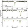 |
Fig. 11 Same as Fig. 10 but for NLTE models with solar (red line) and LTE abundances (green line). |
| In the text | |
|
Fig. 12 NLTE models with solar (red line) and LTE abundances (green line) of the Si iii triplet. |
| In the text | |
Current usage metrics show cumulative count of Article Views (full-text article views including HTML views, PDF and ePub downloads, according to the available data) and Abstracts Views on Vision4Press platform.
Data correspond to usage on the plateform after 2015. The current usage metrics is available 48-96 hours after online publication and is updated daily on week days.
Initial download of the metrics may take a while.