| Issue |
A&A
Volume 545, September 2012
|
|
|---|---|---|
| Article Number | A50 | |
| Number of page(s) | 9 | |
| Section | Numerical methods and codes | |
| DOI | https://doi.org/10.1051/0004-6361/201219076 | |
| Published online | 05 September 2012 | |
Fast calculation of the Lomb-Scargle periodogram using nonequispaced fast Fourier transforms
LESIA, Observatoire de Paris, CNRS, UPMC, Université
Paris-Diderot, 5 place Jules
Janssen, 92195
Meudon, France
e-mail: This email address is being protected from spambots. You need JavaScript enabled to view it.
Received:
20
February
2012
Accepted:
23
July
2012
Abstract
We present a code for the fast computation of the Lomb-Scargle periodogram that uses nonequispaced fast Fourier transforms (FFTs). The computation time has the classical O(Nlog N) behaviour of FFTs, but is shorter by about one order of magnitude than the “classical” fast algorithm by Press and Rybicki, and is about five times shorter that the best GPU-based implementations of the usual O(N2) algorithm. This performance is achieved without sacrificing accuracy, as revealed by comparing the computations done with our FFT-based algorithm and a naïve one.
Key words: methods: data analysis / methods: numerical / stars: oscillations
© ESO, 2012
1. Introduction
The lightcurves obtained with spatial missions such as CoRoT (Michel et al. 2008) and Kepler (Koch et al. 2010) generally consist of extremely large numbers of samples (typically several hundreds of thousands). In addition, these long times-series cannot be evenly sampled over their full duration (e.g., because of the passage of the spacecraft through radiation belts, or because some CCD pixels may be dead, etc.). As a result, the search for periods in the lightcurves cannot be made with direct recourse to the fast Fourier transform (FFT).
In the presence of a nonuniformly sampled lightcurve, it is not uncommon to transform it by interpolation into one with a uniform sampling before doing spectral analysis via FFT. This, however, is not entirely satisfactory since it modifies the statistical properties of the data by introducing artificial data.
One of the most popular alternatives is the accelerated computation of the Lomb-Scargle periodogram proposed by Press & Rybicki (1989), which dramatically improves, in terms of running time, on the original periodogram developed by Lomb (1976) and Scargle (1982). Interestingly, the basic idea behind the Lomb-Scargle periodogram was originally presented in Gottlieb et al. (1975). Though this results in the evaluation of an approximation to the periodogram, it has been generally adopted not only because it is fast, but also because it retains a good accuracy. Another approach was proposed by Townsend (2010), where instead of evaluating an approximation, the exact periodogram is evaluated by leveraging the computing power of graphics processing units (GPUs). In spite of relying on a O(N2) algorithm (where N is the number of samples), this runs on a state-of-the art GPU and is slightly faster than the “classical” O(Nlog N) algorithm by Press & Rybicki on a conventional processor (CPU).
In this paper, we propose to evaluate an approximation to the Lomb-Scargle periodogram by taking advantage of comparatively recent algorithms developed for the fast calculation of Fourier transforms of nonuniformly sampled times-series. Thus, we use the software library developped by Keiner et al. (2009), namely the library of nonequispaced FFTs (NFFTs). The computational time scales with the number of data samples, N, practically as O(Nlog N) (for the details, see Keiner et al. 2009); however, the implied constant in the O-notation is smaller than that of Press & Rybicki mainly owing to the use the state-of-the-art FFT implementation in the FFTW library (Frigo & Johnson 2005). The accuracy of the NFFT is excellent (Steidl 1998).
The paper is organised as follows. In Sect. 2, we briefly recall the formalism of the Lomb-Scargle periodogram. Section 3 introduces the general ideas behind the NFFT algorithms. A code for computing an NFFT-based periodogram is presented in Sect. 4. Benchmarking computations and comparisons with existing codes are presented in Sect. 5. Finally, several perspectives are outlined in Sect. 6.
2. The Lomb-Scargle periodogram
Here we give a brief overview of the formalism of the Lomb-Scargle periodogram. Given a set
of N measurements yi at
observation times
ti (i = 1,...,N),
the Lomb-Scargle normalised periodogram at frequency f is
defined as (Press & Rybicki 1989) ![Mathematical equation: \begin{eqnarray} \label{eq:periodo}\nonumber P_N(f) & = &\frac{1}{2\sigma^2} \left\{ \frac{\left[\sum_i(y_i - \bar{y}) \cos \omega(t_i - \tau)\right]^2} {\sum_i \cos^2 \omega(t_i - \tau)} \right. \\ && \left. + \frac{\left[\sum_i(y_i - \bar{y}) \cos \omega(t_i - \tau)\right]^2} {\sum_i \cos^2 \omega(t_i - \tau)} \right\}, \end{eqnarray}](/articles/aa/full_html/2012/09/aa19076-12/aa19076-12-eq9.png) (1)where
ω = 2πf,
(1)where
ω = 2πf,  ,
and σ2 are the mean and variance of the measurements,
respectively, given by
,
and σ2 are the mean and variance of the measurements,
respectively, given by  (2)and the time-offset τ is
defined by
(2)and the time-offset τ is
defined by  (3)Here and throughout this section, the
summations run from i = 1 to i = N.
(3)Here and throughout this section, the
summations run from i = 1 to i = N.
Scargle (1982) and Schwarzenberg-Czerny (1998) investigated the statistical distribution of the
periodogram under the assumption that the measurements originate from pure Gaussian white
noise. Schwarzenberg-Czerny (1998) showed that, in
this case, a periodogram, normalised by the total variance as in Eq. (1), follows a Beta distribution
Ix [1,(N − 3)/2] , defined
as  (4)with
x = 2PN(f)/N,
and where B(a,b) and Bx(a,b)
are, respectively, the Beta function and the incomplete version thereof, defined as (NIST 2011)
(4)with
x = 2PN(f)/N,
and where B(a,b) and Bx(a,b)
are, respectively, the Beta function and the incomplete version thereof, defined as (NIST 2011)
 (5)In the case of Gaussian white noise, the
false-alarm probability that a periodogram comprising M independent
frequencies will exhibit a peak due to chance fluctuations is
(5)In the case of Gaussian white noise, the
false-alarm probability that a periodogram comprising M independent
frequencies will exhibit a peak due to chance fluctuations is ![Mathematical equation: \begin{eqnarray} \label{eq:fap} \nonumber P_{\mathrm{FA}} &=& 1 - \left[1 - I_x\left(1, \frac{N-3}{2}\right)\right]^M \\[2mm] &=& 1 - \left[1 - \left(1 - \frac{2P_N(f)}{N}\right)^{(N-3)/2}\right]^M \cdot \end{eqnarray}](/articles/aa/full_html/2012/09/aa19076-12/aa19076-12-eq25.png) (6)The non-trivial question of whether we can
determine the number of independent frequencies in a periodogram has been addressed in the
literature (Horne & Baliunas 1986; Frescura et al. 2008), and is not considered here because
that would be beyond the scope of this paper.
(6)The non-trivial question of whether we can
determine the number of independent frequencies in a periodogram has been addressed in the
literature (Horne & Baliunas 1986; Frescura et al. 2008), and is not considered here because
that would be beyond the scope of this paper.
As noted by Press & Rybicki (1989), the sums
that occur in Eq. (1) can be greatly
simplified. If we define ![Mathematical equation: \begin{equation} \label{eq:defsums} \begin{array}{ll} \displaystyle S_y = \sum_i(y_i-\bar{y}) \sin\omega t_i , & \displaystyle C_y = \sum_i(y_i-\bar{y}) \cos\omega t_i , \\[2mm] \displaystyle S_2 = \sum_i \sin 2\omega t_i , & \displaystyle C_2 = \sum_i \cos 2\omega t_i , \end{array} \end{equation}](/articles/aa/full_html/2012/09/aa19076-12/aa19076-12-eq26.png) (7)then
(7)then ![Mathematical equation: \begin{eqnarray} && \displaystyle \sum_i(y_i-\bar{y})\cos\omega(t_i-\tau) = C_y\cos\omega\tau + S_y\sin\omega\tau, \nonumber\\[2mm] && \displaystyle \sum_i(y_i-\bar{y})\sin\omega(t_i-\tau) = S_y\cos\omega\tau - C_y\sin\omega\tau, \nonumber\\[2mm] && \displaystyle \sum_i\cos^2\omega(t_i-\tau) = \frac{N}{2} + \frac{1}{2}C_2\cos 2\omega\tau + \frac{1}{2}S_2\sin 2\omega\tau, \nonumber\\[2mm] && \displaystyle \sum_i\sin^2\omega(t_i-\tau) = \frac{N}{2} - \frac{1}{2}C_2\cos 2\omega\tau \label{eq:sums} - \frac{1}{2}S_2\sin 2\omega\tau. \end{eqnarray}](/articles/aa/full_html/2012/09/aa19076-12/aa19076-12-eq27.png) (8)These simplifications form the basis of the
code proposed in Press et al. (1992). These authors
emphasised that if the ti were evenly spaced,
the above sums could be evaluated by two complex FFTs before substituting them back into
Eqs. (1) and (3). To be able to use FFTs despite the nonuniformity of the
ti, they invented the so-called
extirpolation process, which is based on the Lagrange interpolation (see
their paper for details). Here, we instead propose to bypass the extirpolation process, and
to directly compute the sums given in Eq. (8)
by using complex NFFTs, since a new numerical tool to evaluate these now exists under the
form of a freely available, high-quality library written in C language (Keiner et al. 2009).
(8)These simplifications form the basis of the
code proposed in Press et al. (1992). These authors
emphasised that if the ti were evenly spaced,
the above sums could be evaluated by two complex FFTs before substituting them back into
Eqs. (1) and (3). To be able to use FFTs despite the nonuniformity of the
ti, they invented the so-called
extirpolation process, which is based on the Lagrange interpolation (see
their paper for details). Here, we instead propose to bypass the extirpolation process, and
to directly compute the sums given in Eq. (8)
by using complex NFFTs, since a new numerical tool to evaluate these now exists under the
form of a freely available, high-quality library written in C language (Keiner et al. 2009).
3. The NFFT algorithm and library
We present the principles of the computation of an NFFT, to ensure that the library implementing it does not appear as a mere black box, and that motivated users will be able to understand and adjust the fine tunings offered by the library.
If a continuous signal y(t) is sampled every
Δt seconds at N observation times
tj = jΔt (j = 0,...,N − 1),
a time series
yj = y(tj)
is obtained. Its discrete Fourier transform is defined as 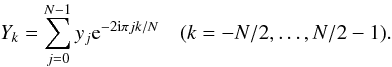 (9)The domain of k is written so
as to reflect that there are only N independent discrete frequencies
fk = k/(NΔt),
and that these satisfy
(9)The domain of k is written so
as to reflect that there are only N independent discrete frequencies
fk = k/(NΔt),
and that these satisfy  (10)where
fc = 1/(2Δt) is the Nyquist
frequency. The inverse transform is
(10)where
fc = 1/(2Δt) is the Nyquist
frequency. The inverse transform is  (11)The mathematicians who developed the
NFFT (Keiner et al. 2009) define the
nonequispaced discrete Fourier transform (NDFT) as the generalisation of
Eq. (11) without the normalising constant
(11)The mathematicians who developed the
NFFT (Keiner et al. 2009) define the
nonequispaced discrete Fourier transform (NDFT) as the generalisation of
Eq. (11) without the normalising constant
 (12)where the complex quantities
Yk are given,
xj, are reduced times, called
nodes, satisfying
−1/2 ≤ xj < 1/2, and one does not
necessarily have M = N. (If N is odd, the
summation runs from − [N/2] to [N/2] , where the
brackets mean the integer part.) This can be written in matrix-vector notation as
(12)where the complex quantities
Yk are given,
xj, are reduced times, called
nodes, satisfying
−1/2 ≤ xj < 1/2, and one does not
necessarily have M = N. (If N is odd, the
summation runs from − [N/2] to [N/2] , where the
brackets mean the integer part.) This can be written in matrix-vector notation as
 (13)where A is a complex
M × N matrix
(Ajk = e−2iπkxj).
This matrix is generally not square, and had it been so, it would generally be neither
orthogonal nor invertible. The definition of the inverse NDFT is therefore a complicated
issue. It is, instead, customary to consider the adjoint NDFT defined by
(13)where A is a complex
M × N matrix
(Ajk = e−2iπkxj).
This matrix is generally not square, and had it been so, it would generally be neither
orthogonal nor invertible. The definition of the inverse NDFT is therefore a complicated
issue. It is, instead, customary to consider the adjoint NDFT defined by
 (14)where AH is the adjoint
(or conjugate transpose) of matrix A. This corresponds to the sums
(14)where AH is the adjoint
(or conjugate transpose) of matrix A. This corresponds to the sums
 (15)which is the customary formulation needed for
the computation of a periodogram.
(15)which is the customary formulation needed for
the computation of a periodogram.
In view of the duality expressed by Eqs. (13) and (14), it turns out that the same methods can be applied to compute the sums in Eqs. (12) and (15).
The NFFT is an efficient computation of the NDFT defined in Eq. (12). To this end, the trigonometric polynomial
 (16)is first approximated by suitable linear
combinations of translates of a window function ϕ having good localization
in time/space and frequency1. The function
y(x) in Eq. (16) is periodic and has a period equal to 1, therefore the function
ϕ(x), too, is chosen to be 1-periodic. Introducing an
oversampling factor σ > 1 and setting
n = σN, y(x) is
approximated by
(16)is first approximated by suitable linear
combinations of translates of a window function ϕ having good localization
in time/space and frequency1. The function
y(x) in Eq. (16) is periodic and has a period equal to 1, therefore the function
ϕ(x), too, is chosen to be 1-periodic. Introducing an
oversampling factor σ > 1 and setting
n = σN, y(x) is
approximated by  (17)The question is then to define
gl such that
s1 ≈ y. Converting the right-hand side of
Eq. (17) to the frequency domain yields
(17)The question is then to define
gl such that
s1 ≈ y. Converting the right-hand side of
Eq. (17) to the frequency domain yields
 (18)where
  (19)and
  (20)If Φ(k) becomes sufficiently
small for |k| > n/2 and if Φ(k) ≠ 0
for −n/2 ≤ k < n/2, then comparison of
Eqs. (16) and (18) suggests that one defines
ĝk such that
(20)If Φ(k) becomes sufficiently
small for |k| > n/2 and if Φ(k) ≠ 0
for −n/2 ≤ k < n/2, then comparison of
Eqs. (16) and (18) suggests that one defines
ĝk such that  (21)From Eq. (19), gl is now given by
 (22)which can be computed by an FFT of length
n. If ϕ is also localised in the time domain, so that it
can be approximated by a 1-periodic function ψ
(22)which can be computed by an FFT of length
n. If ϕ is also localised in the time domain, so that it
can be approximated by a 1-periodic function ψ![Mathematical equation: \begin{equation} \label{eq:psi} \psi(x) = \varphi(x) \chi_{[-m/n,m/n]}(x) \qquad (m < n, m\in\mathbb{N}), \end{equation}](/articles/aa/full_html/2012/09/aa19076-12/aa19076-12-eq74.png) (23)where m is a cutoff parameter
and
χ [−m/n,m/n] (x)
is the characteristic function defined as
(23)where m is a cutoff parameter
and
χ [−m/n,m/n] (x)
is the characteristic function defined as
![Mathematical equation: \begin{equation} \chi_{[-m/n,m/n]} (x) = \left\{ \begin{array}{ll} 1, &\quad -m/n \le x \le m/n, \\ 0, &\quad \mbox{otherwise}, \end{array} \right. \end{equation}](/articles/aa/full_html/2012/09/aa19076-12/aa19076-12-eq77.png) (24)then an approximation to
s1 is defined by
(24)then an approximation to
s1 is defined by ![Mathematical equation: \begin{equation} \label{eq:trunc} s(x_j) = \sum_{l = -n/2}^{n/2-1} g_l \psi(x_j - l/n) = \sum_{l=[nx_j] - m}^{[nx_j] + m} g_l \psi(x_j - l/n). \end{equation}](/articles/aa/full_html/2012/09/aa19076-12/aa19076-12-eq79.png) (25)To summarise, one has
(25)To summarise, one has  (26)which translates into the following three-step
algorithm. Given a suitably chosen window function ϕ, we (i) compute
Gk according to Eq. (21); (ii) compute the Fourier transform of
Gk using FFT, which is efficiently achieved
with the help of the FFTW library (Frigo & Johnson
2005); (iii) compute the sum
s(xj) of Eq. (25). Each of these three steps is linear and can
be conveniently represented by a matrix (respectively, D, F, and
B), so that Eq. (13) reads
(26)which translates into the following three-step
algorithm. Given a suitably chosen window function ϕ, we (i) compute
Gk according to Eq. (21); (ii) compute the Fourier transform of
Gk using FFT, which is efficiently achieved
with the help of the FFTW library (Frigo & Johnson
2005); (iii) compute the sum
s(xj) of Eq. (25). Each of these three steps is linear and can
be conveniently represented by a matrix (respectively, D, F, and
B), so that Eq. (13) reads
 (27)As noted earlier, for the computation of a
periodogram we actually need the adjoint NFFT, i.e.,
(27)As noted earlier, for the computation of a
periodogram we actually need the adjoint NFFT, i.e.,  (28)This is essentially the same algorithm taken in
reverse order, therefore its performances are the same as that for the direct NFFT. In
particular, the arithmetical complexity of the algorithm can be shown to be
O(Nlog N + M) (Keiner et al. 2009).
(28)This is essentially the same algorithm taken in
reverse order, therefore its performances are the same as that for the direct NFFT. In
particular, the arithmetical complexity of the algorithm can be shown to be
O(Nlog N + M) (Keiner et al. 2009).
In addition, we note that the two approximations in Eq. (26) introduce, respectively, an aliasing error and a truncature error, both of which could be rigorously analysed for various window functions (e.g. Potts et al. 1998). This contrasts with several of the earlier NFFT algorithms.
The above NFFT algorithm and its adjoint are efficiently implemented in the NFFT library (Keiner et al. 2009), written in C language and freely downloadable2. This library is not limited to one-dimensional Fourier transforms that are nonequispaced in time, and provides a large bestiary of transforms in several dimensions; in particular, the case nonequispaced in both time and frequency is considered. The library also provides iterative methods to compute the corresponding inverse transforms. Moreover, several of the more important window functions considered in the literature are implemented, and their parameters have default values that yield smaller aliasing and truncating errors.
4. An NFFT-based Lomb-Scargle periodogram code
We now present nfftls, a code for computing a Lomb-Scargle periodogram that is a straightforward implementation of Eq. (1) rewritten in terms of the sums in Eq. (8) computed using NFFTs.
The periodogram is output on a uniform frequency grid  (29)where the frequency spacing is given by
 (30)Cover is an
oversampling parameter3, and the number of frequencies
is
(30)Cover is an
oversampling parameter3, and the number of frequencies
is  (31)The control parameter
Chigh is the ratio of the highest desired frequency,
fhigh, to the Nyquist frequency,
fc = Nt/(2T),
that would be obtained if the Nt data points
were evenly sampled over the total sampling time
T = tNt − t1.
The oversampling parameter and the high frequency parameter are both user inputs. It should
be emphasised that in practice the choice of these parameters must be guided by the data
sampling and the scientific problem at hand.
(31)The control parameter
Chigh is the ratio of the highest desired frequency,
fhigh, to the Nyquist frequency,
fc = Nt/(2T),
that would be obtained if the Nt data points
were evenly sampled over the total sampling time
T = tNt − t1.
The oversampling parameter and the high frequency parameter are both user inputs. It should
be emphasised that in practice the choice of these parameters must be guided by the data
sampling and the scientific problem at hand.
As mentioned in Sect. 3, the NFFT library assumes that
the time range is the interval [−1/2,1/2); therefore, before the computation of the NFFTs,
the original time range must be mapped to this interval. This is achieved by applying the
following transformation  (32)with
  , where ϵ is an arbitrarily
small number (typically 10-5).
, where ϵ is an arbitrarily
small number (typically 10-5).
Figure A.1 lists the C99 code for the computation of the Fourier transform of an unevenly sampled times-series with the help of the NFFT library. We note that, owing to the implementation of the library, not the direct transform (Eq. (12)), but the adjoint transform (Eq. (15)) must be computed. Moreover, we note that the Fourier transform is not normalised. Though the function computes the transform at all frequencies −mδf ≤ f ≤ mδf (with m = Nf), it outputs only the positive frequency part, since only strictly positive frequencies are involved in the computation of the periodogram.
For the computation of the transforms in Eq. (7) at angular frequencies 2ω, it suffices to compute a Fourier
transform of the observational window (i.e., with the data samples equal to 1.0) that is
twice as long as that of the data 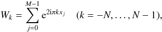 (33)and to take every second Fourier component. It
turns out that the extra calculation that needs to be made negligly affects the time
performances of the code.
(33)and to take every second Fourier component. It
turns out that the extra calculation that needs to be made negligly affects the time
performances of the code.
The outline of the program is then very simple:
-
1.
Read the input data (times-series).
-
2.
Compute the mean and the variance of the data.
-
3.
Centre the data around their mean.
-
4.
Reduce the time span to the interval [−1/2,1/2), taking oversampling into account (Eq. (32)).
-
5.
Determine the maximum frequency element to be output.
-
6.
Compute the Fourier transform of the data (Eq. (15) expressed in NFFT terms as Eq. (28)).
-
7.
Compute the Fourier transform (of double length) of the window (Eq. (33) expressed as Eq. (28) where y has all its components equal to unity).
-
8.
Compute the sums of Eq. (8), then the periodogram (Eq. (1)).
-
Output the periodogram.
-
10.
Output false-alarm probability (Eq. (6)) vs. frequency (optional).
We note that steps 5 to 8 are actually wrapped into a C function that returns a C-structure containing the two arrays that make up the periodogram, viz. the frequencies and the corresponding periodogram ordinates. Figure A.2 lists the code of that function.
5. Tests and comparisons with existing codes
The tests were conducted on two platforms. One is a laptop Dell Latitude E6400 that runs 64-bit Ubuntu GNU/Linux, with 3 GB of RAM. It has an Intel(R) Core(TM)2 Duo P9700 Processor, with a cache size of 6 MB and a clock speed of 2.8 GHz. The other one is a 64-bit Debian GNU/Linux server with 47 GB of RAM. It has four hexa-core Intel(R) Xeon(R) Processors X5650, each with a cache size of 12 MB and a clock speed of 2.66 GHz. No attempt was made to parallelise the code, and the program was run on only one core of a single chip. Hence, as the clock speeds of both platforms are quite similar, the running times of the same program executed on them essentially differ because of the effects of the cache and RAM sizes. The executables were created on both machines with the GNU gcc compiler (v4.6.1 for the laptop and v4.4.5 for the server), using the standard C99 language (option -std=c99) and the -O2 optimization flag.
For the validation of our code nfftls, we used several sets of simulated data, regularly as well as irregularly sampled, some with gaps. We compared the results with a code based on a straightforward implementation of the DFT, which is hence very slow because it is based on a O(N2) algorithm. The maximal absolute deviation between the results of both codes was found to be of the order of 10-8. In addition, the presence of gaps in the data or a random sampling did not alter the performances of nfftls, in terms of neither runtime nor numerical accuracy.
For the performance comparisons, we used the following codes: fasper, the fast algorithm proposed by Press & Rybicki (1989), in its C version (Press et al. 1992), and culsp the GPU-based algorithm proposed by Townsend (2010).
One should be aware that the GPU-based algorithm, culsp, is a straightforward implementation of exact expressions for the Fourier transforms, whilst fasper and nfftls are both implementations of approximate expressions thereof (reverse interpolation or extirpolation in fasper, and those summarised by Eq. (26), and described in Sect. 3, in nfftls) in order to take advantage of the FFT.
To compare the performances of our code to Townsend’s culsp 2010, we used the same validation data set, namely the 150-day photometric time-series of the large-amplitude β Cephei pulsator V1449 Aql (HD 180642) obtained by the CoRoT mission4 (Belkacem et al. 2009). After removal of the flux measurements flagged as bad, the times-series comprised 382 003 points, unevenly sampled. Whilst the sampling of the data set is mostly regular (with a sampling interval of about 32 s), there are gaps of various sizes (see Fig. 1).
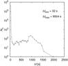 |
Fig. 1 Histogram of the sampling intervals in the V1149 Aql data set. The number of sampling intervals, NΔ, of a given value, Δt, is plotted only up to Δt = 2000 s; the maximal sampling interval is a huge gap of Δtmax = 9504 s. The minimal sampling interval Δtmin = 32 s corresponds to the nominal observation mode. |
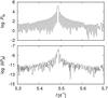 |
Fig. 2 Upper plot: part of the L-S periodogram for V1449 Aql; lower
plot: absolute deviation |

The periodogram of V1449 Aql was computed with nfftls. Figure 2 (upper plot) displays the part surrounding the peak corresponding to the
dominant 0.18 d pulsation period (Waelkens et al.
1998). To get an idea of the accuracy, we also computed the periodogram using an
implementation of the DFT that is a straightforward translation of Eq. (15). Figure 3 shows a scatter plot of the straightforward DFT- and NFFT-based periodograms
against one another over the full frequency range. The good agreement between both codes is
clear: no point in the plot departs from the diagonal line
 , the maximal absolute “error” is
 (see lower plot in Fig. 2), and the corresponding relative “error” is of the order of
10-13. This illustrates that the approximation performed by the NFFT-based code
in computing a periodogram is extremely good. We note that a relative error of about that
same size is measured when comparing the absolute value of a DFT computed without recourse
to the FFT and one computed by using the NFFT library. All computations were done in double
precision.
(see lower plot in Fig. 2), and the corresponding relative “error” is of the order of
10-13. This illustrates that the approximation performed by the NFFT-based code
in computing a periodogram is extremely good. We note that a relative error of about that
same size is measured when comparing the absolute value of a DFT computed without recourse
to the FFT and one computed by using the NFFT library. All computations were done in double
precision.
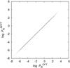 |
Fig. 3 Scatter plot of the NFFT-based periodogram against the straightforward DFT-based periodogram for V1449 Aql. |
Periodogram computation times in seconds.
To measure the performance of nfftls and ease the comparison, we adopted Townsend’s approach. We averaged the periodogram computation time over 100 runs (the typical running time for one computation is so short, that repetition was necessary). To make a fair comparison, we took into consideration only the time necessary to execute steps 5 to 8 (inclusive) of the code outline given in Sect. 4. Table 1 lists the mean periodogram computation time ⟨ tcalc ⟩ and the corresponding standard deviation σ(tcalc) for nfftls running on both the laptop and the server; for comparison, we also list the performances of a code based on fasper and Townsend’s code culsp. We modified the function fasper by Press et al. (1992) by introducing instructions for timing the code at places most similar to those they have in nfftls, so that the comparison of running times was as fair as possible. In addition, we note that the computations in fasper are done essentially in single precision, whilst they are done in double precision in nfflts. The use of single precision generally seriously impairs the accuracy, and depending on the computer architecture, the running time may also be affected5. We note that if the running time values for nfftls are corrected by adding the time necessary for executing steps 2 to step 4, this amounts to increasing the corresponding tabulated values by ~8 ms, which is negligible.
Townsend’s platform has a clock frequency of 2.33 GHz, which is not very different from that of our platforms (2.67 GHz and 2.80 GHz), therefore one may infer that the running times of nfftls and fasper on his platform would be comparable to that displayed in Table 1 (the RAM size of Townsend’s platform is 8 GB, hence bracketed by the RAM sizes of our platforms).
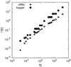 |
Fig. 4 Running time as a function of the length of the times-series of fasper and nfftls. The dotted straight line is a least squares fit with a function proportional to Ntlog Nt. |
Figure 4 plots the running time of fasper and nfftls as a function of the length Nt of the times-series. The times-series for a given Nt is obtained by downsampling the original one. Although both are O(Ntlog Nt) codes, clearly, the latter runs faster, viz. at least about six times faster, as indicated in Table 1. This difference in performance may be ascribed in large part to the implementation of the FFT on which both codes rest, and in particular to the use of the FFTW library in computing NFFTs.
In addition, nffls outperforms the GPU-based codes, typically running about four times faster than a code running on a Tesla C1060, one of the upper-end GPUs available on the market. Moreover, the computation with GPUs are still limited to a single precision accuracy, whilst codes running on CPUs can benefit from the built-in double precision of the standard C libraries. This presumably explains the great difference in the relative errors registered by nfftls and culsp. As far as the computation of periodogram ordinates is concerned, this should not be too great a problem since the relative errors are very small in both cases. In this context, the most important considerations are the good performances in terms of running time.
Finally, we note that we found no improvement could be achieved by changing the default settings of the NFFT library, namely by departing from the Kaiser-Bessel window function (Jackson et al. 1991; Fourmont 1999) and/or by modifying default values of the parameters that control the quality of the NFFT approximation (viz. the “internal” oversampling and the cutoff parameter mentioned in Sect. 3).
6. Conclusions and perspectives
We have shown that the use of NNFTs could significantly shorten the running time for computing the periodogram of nonuniformly sampled light curves whilst ensuring an excellent accuracy. This, of course, assumes that the libraries used provide state-of-the-art implementations of the FFT and of the NFFTs. In this respect, the quality of the treatment of the approximations done by Keiner et al. (2009) in computing NFFTs makes their library highly commendable.
One should be aware that, for the mass treatment of the many stars for which space missions are now providing very long lightcurves, even a gain in running time of about one order of magnitude, as we obtain, over the “classical” accelerated algorithm by Press & Rybicki (1989) is a valuable improvement. In addition, not only periodogram-orientated programs but virtually any spectral analysis program that must deal with irregularly sampled data could benefit from using NFFTs.
For example, Scargle (1989) discusses in detail Fourier transforms and correlation functions of irregularly sampled data, but provides an implementation of the DFT based on a O(N2) algorithm, which is therefore virtually impractical for very long times-series. Nothing in his discussion, however, prevents the replacement of his implementation with an NFFT, which would result in a dramatic decrease in running time. To this end, the implementation given in Fig. A.1 may serve as a guide. At this point, we wish to mention that the inversion back to the time domain performed by taking the FFT of a DFT evaluated at evenly spaced frequencies, as proposed by Scargle, might be replaced with the use of one of the iterative solvers proposed by Keiner et al. (2009) in their NFFT library; typically, a solver iteratively solves, e.g., Eq. (13) for Y given y.
Among the various programs that may greatly benefit from the use of NFFTs, we only mention the one that is most used in stellar astronomy: sigspec by Reegen (2007). Though an extremely effective tool, it is terribly slow because it does not make any recourse to the use of FFTs. Unfortunately, the complexity of the source code and its author’s death make the corresponding adaptation a challenging (though certainly worthwhile) task.
In view of the already very good performances reached in computing an NFFT-based periodogram on a single processor core, it will be interesting to investigate whether parallelism may bring further improvement. We note that there have been some recent developments (Pippig 2009) towards producing a parallel version of the NFFT library6. However, we find that the available software remains insufficiently robust for it to serve as a basis for a code delivered to a large community.
The general trends in computer technology is not only towards multicore CPUs but also towards programmable GPUs. In addtion, computations of NFFTs on GPUs have started to appear (Sørensen et al. 2008). However, GPU computing remains too hardware-dependent, and monothread CPU computing is much easier to program7.
We therefore believe that the excellent performances that can be obtained with monothread computing using high-quality libraries, such as the FFTW and NFFT libraries, should continue to make codes such as nfftls extremely attractive.
The approximation of a function by translates of a basis function is a well-known method in approximation theory (e.g. Schaback 1995).
Note that this oversampling parameter has nothing to do with the “internal” parameter of the same name used in the NFFT approximation.
The CoRoT space mission, launched on 2006 December 27, was developed and is operated by the CNES, with participation of the Science Programs of ESA, ESA’s RSSD, Austria, Belgium, Brazil, Germany, and Spain.
In C, this generally results in an increase in running time since the mathematical libraries for this language are in double precision.
But this situation may change in a near future, as Intel recently (Aug. 2011) announced they are porting their Cilk Plus C/C++ language extensions for multithreaded parallel computing into the GNU Compiler collection (http://software.intel.com/en-us/articles/intel-cilk-plus-open-source/).
References
- Belkacem, K., Samadi, R., Goupil, M.-J., et al. 2009, Science, 324, 1540 [NASA ADS] [CrossRef] [Google Scholar]
- Fourmont, K. 1999, Ph.D. Thesis, Mathematisch-Naturwissenschaftlichen Fakulät der Westfälischen Wilhelms-Universität Münster, Germany [Google Scholar]
- Frescura, F. A. M., Engelbrecht, C. A., & Frank, B. S. 2008, MNRAS, 388, 1693 [NASA ADS] [CrossRef] [Google Scholar]
- Frigo, M., & Johnson, S. G. 2005, Proc. IEEE, 93, 216 [Google Scholar]
- Gottlieb, E. W., Wright, E. L., & Liller, W. 1975, ApJ, 195, L33 [NASA ADS] [CrossRef] [Google Scholar]
- Horne, J. H., & Baliunas, S. L. 1986, ApJ, 302, 757 [NASA ADS] [CrossRef] [Google Scholar]
- Jackson, J. I., Meyer, C. H., Nishimura, D. G., & Macovski, A. 1991, IEEE Trans. Med. Imag., 10, 473 [Google Scholar]
- Keiner, J., Kunis, S., & Potts, D. 2009, ACM Trans. Math. Softw., 36, 1 [Google Scholar]
- Koch, D. G., Borucki, W. J., Basri, G., et al. 2010, ApJ, 713, L79 [NASA ADS] [CrossRef] [Google Scholar]
- Lomb, N. R. 1976, Ap&SS, 39, 447 [NASA ADS] [CrossRef] [Google Scholar]
- Michel, E., Baglin, A., Weiss, W. W., et al. 2008, Commun. Asteroseismol., 156, 73 [NASA ADS] [CrossRef] [Google Scholar]
- NIST 2011, Digital Library of Mathematical Functions, National Institute of Standards and Technology, Release date: 2011-08-29, http://dlmf.nist.gov/ [Google Scholar]
- Pippig, M. 2009, Ph.D. Thesis, Chemnitz University of Technology [Google Scholar]
- Potts, D., Steidl, G., & Tasche, M. 1998, in Modern Sampling Theory: Mathematics and Applications, eds. J. Benedetto, & P. Ferreira, 249 [Google Scholar]
- Press, W. H., & Rybicki, G. B. 1989, ApJ, 338, 277 [NASA ADS] [CrossRef] [Google Scholar]
- Press, W. H., Tukolsky, S. A., Vetterling, W. T., & Flannery, B. P. 1992, Numerical Recipes in C: The Art of Scientific Computing, 2nd edn. (Cambridge University Press) [Google Scholar]
- Reegen, P. 2007, A&A, 467, 1353 [NASA ADS] [CrossRef] [EDP Sciences] [Google Scholar]
- Scargle, J. D. 1982, ApJ, 263, 835 [NASA ADS] [CrossRef] [Google Scholar]
- Scargle, J. D. 1989, ApJ, 343, 874 [NASA ADS] [CrossRef] [Google Scholar]
- Schaback, R. 1995, in Approximation Theory VIII, Vol. 1: Approximation and Interpolation, eds. C. Chui, & L. Schumaker (World Scientific Publishing Co., Inc.), 491 [Google Scholar]
- Schwarzenberg-Czerny, A. 1998, MNRAS, 301, 831 [NASA ADS] [CrossRef] [Google Scholar]
- Sørensen, T. S., Schaeffer, T., Noe, K. O., & Hansen, M. 2008, IEEE Trans. Med. Imag., 27, 538 [CrossRef] [Google Scholar]
- Steidl, G. 1998, Adv. Comput. Math., 9, 337 [CrossRef] [Google Scholar]
- Townsend, R. H. D. 2010, ApJS, 191, 247 [NASA ADS] [CrossRef] [Google Scholar]
- Waelkens, C., Aerts, C., Kestens, E., Grenon, M., & Eyer, L. 1998, A&A, 330, 215 [NASA ADS] [Google Scholar]
Appendix A: C-code for computing a periodogram
In this appendix, we introduce the two building blocks necessary for computing a normalised Lomb-Scargle periodogram by using NFFTs. The complete program, nfftls, is freely available, under the GNU General Public License (GPLv3)8.
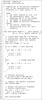 |
Fig. A.1 Function for computing an NFFT. |
Figure A.1 presents the function, nfft, that computes the NFFT of a times-series (the so-called dirty spectrum) or the corresponding observational window. To compute the latter, a NULL pointer must be provided as the argument for the measurements.
If the appropriate flags in the nnft_plan are set after it has been initialised
(line 26), an optimisation is obtained by precomputing the values of
 for k = −N/2,...,/N2−1
(Eq. (20)). The library’s default
settings are such that the test on line 46 evaluates to true, so that another optimisation
is done by precomputing (line 47) the values of
ψ(xj − l/n)
for j = 1,...,M and
l = [nxj] − m,..., [nxj] + m
(Eq. (25)). We tried to improve the
performance by varying these flags, but did not find any significant difference in the
code performance. The library’s defaults seem to conform perfectly to our needs. For more
details on the available optimisations, the reader is referred to Keiner et al. (2009).
for k = −N/2,...,/N2−1
(Eq. (20)). The library’s default
settings are such that the test on line 46 evaluates to true, so that another optimisation
is done by precomputing (line 47) the values of
ψ(xj − l/n)
for j = 1,...,M and
l = [nxj] − m,..., [nxj] + m
(Eq. (25)). We tried to improve the
performance by varying these flags, but did not find any significant difference in the
code performance. The library’s defaults seem to conform perfectly to our needs. For more
details on the available optimisations, the reader is referred to Keiner et al. (2009).
Figure A.2 presents the function periodogram used to compute the periodogram proper. Before the call, the user must have centred the measurements around their mean, and the observation times must have been reduced so as to lie in the interval [−1/2,1/2). The function returns the results in a C-structure, LS, defined as
            typedef struct  {
               double* freqs; //   (>0)   frequencies
               double* Pn;   //   periodogram ordinates
               int nfreqs;   //    number of frequencies
            } LS;
whose members are labelled freqs and Pn are two dynamically allocated arrays of size nfreqs. This structure is allocated by the function itself (lines 26−29); it is however the responsibility of the user to free the corresponding memory.
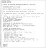 |
Fig. A.2 Function for computing an NFFT-based LS periodogram. |
The undisplayed header file declar.h (line 3) contains the declarations of the function nfft as well as of the auxiliary functions
-
sign (line 48), which transfers the sign of itssecond argument to its first argument, i.e. sign(a, b) returns |a|sgnb,where sgn(x) yields the sign of x ;
-
square (lines 50−51), which returns the square of its argument;
-
xmalloc (lines 26–28, 32, 35), which is a wrapper of the standard function malloc that terminates the program with a message in the case of an error.
In practice, simple functions such as sign and square are inlined in the code.
We note that the function periodogram differs from the function fasper from Numerical Recipes (Press et al. 1992) in two important ways. Firstly, the sums of the trigonometric functions at 2ω in Eq. (7) are evaluated from Fourier transforms of the observational window of a length twice that of the data (lines 36 and 43). Secondly, and more importantly, the Fourier transforms are evaluated as NFFTs (lines 33 and 36). In addition, periodogram does not determine the peak of the maximal height in the periodogram and the corresponding false-alarm probability. In the spirit of the C language, this is instead delegated to another function (not displayed since it is a trivial translation of Eq. (6)).
All Tables
All Figures
|
Fig. 1 Histogram of the sampling intervals in the V1149 Aql data set. The number of sampling intervals, NΔ, of a given value, Δt, is plotted only up to Δt = 2000 s; the maximal sampling interval is a huge gap of Δtmax = 9504 s. The minimal sampling interval Δtmin = 32 s corresponds to the nominal observation mode. |
| In the text | |
|
Fig. 2 Upper plot: part of the L-S periodogram for V1449 Aql; lower
plot: absolute deviation |
| In the text | |
|
Fig. 3 Scatter plot of the NFFT-based periodogram against the straightforward DFT-based periodogram for V1449 Aql. |
| In the text | |
|
Fig. 4 Running time as a function of the length of the times-series of fasper and nfftls. The dotted straight line is a least squares fit with a function proportional to Ntlog Nt. |
| In the text | |
|
Fig. A.1 Function for computing an NFFT. |
| In the text | |
|
Fig. A.2 Function for computing an NFFT-based LS periodogram. |
| In the text | |
Current usage metrics show cumulative count of Article Views (full-text article views including HTML views, PDF and ePub downloads, according to the available data) and Abstracts Views on Vision4Press platform.
Data correspond to usage on the plateform after 2015. The current usage metrics is available 48-96 hours after online publication and is updated daily on week days.
Initial download of the metrics may take a while.