| Issue |
A&A
Volume 545, September 2012
|
|
|---|---|---|
| Article Number | A107 | |
| Number of page(s) | 11 | |
| Section | The Sun | |
| DOI | https://doi.org/10.1051/0004-6361/201015747 | |
| Published online | 14 September 2012 | |
Modelling magnetic flux emergence in the solar convection zone
1
School of Mathematics and Statistics, Newcastle University,
Newcastle Upon Tyne,
NE1 7RU
UK
e-mail: paul.bushby@ncl.ac.uk
2
School of Mathematics and Statistics, University of St. Andrews,
North Haugh, St.
Andrews, Fife
KY16 9SS,
UK
e-mail: vasilis@mcs.st-and.ac.uk
Received:
13
September
2010
Accepted:
29
July
2012
Context. Bipolar magnetic regions are formed when loops of magnetic flux emerge at the solar photosphere. Magnetic buoyancy plays a crucial role in this flux emergence process, particularly at larger scales. However it is not yet clear to what extent the local convective motions influence the evolution of rising loops of magnetic flux.
Aims. Our aim is to investigate the flux emergence process in a simulation of granular convection. In particular we aim to determine the circumstances under which magnetic buoyancy enhances the flux emergence rate (which is otherwise driven solely by the convective upflows).
Methods. We used three-dimensional numerical simulations, solving the equations of compressible magnetohydrodynamics in a horizontally-periodic Cartesian domain. A horizontal magnetic flux tube was inserted into fully developed hydrodynamic convection. We systematically varied the initial field strength, the tube thickness, the initial entropy distribution along the tube axis and the magnetic Reynolds number.
Results. Focusing upon the low magnetic Prandtl number regime (Pm < 1) at moderate magnetic Reynolds number, we find that the flux tube is always susceptible to convective disruption to some extent. However, stronger flux tubes tend to maintain their structure more effectively than weaker ones. Magnetic buoyancy does enhance the flux emergence rates in the strongest initial field cases, and this enhancement becomes more pronounced when we increase the width of the flux tube. This is also the case at higher magnetic Reynolds numbers, although the flux emergence rates are generally lower in these less dissipative simulations because the convective disruption of the flux tube is much more effective in these cases. These simulations seem to be relatively insensitive to the precise choice of initial conditions: for a given flow, the evolution of the flux tube is determined primarily by the initial magnetic field distribution and the magnetic Reynolds number.
Key words: convection / magnetohydrodynamics (MHD) / Sun: interior
© ESO, 2012
1. Introduction
It is generally believed that most of the large-scale toroidal magnetic field in the solar interior is stored in the stably-stratified layer just below the base of the convection zone, where the toroidal field is amplified by the effects of differential rotation (see, for example, Ossendrijver 2003). Through the action of magnetic buoyancy (Parker 1955), segments of this toroidal flux rise into the convection zone, eventually emerging to form bipolar active regions at the solar surface (Zwaan 1985). Several numerical simulations of this flux emergence process have focused upon the interactions between convection and buoyant magnetic flux tubes (Dorch et al. 2001; Fan et al. 2003; Abbett et al. 2004; Stein et al. 2011), whilst others have focused upon the subsequent small-scale and large-scale evolution of the emerging field, as it rises into the photosphere/chromosphere (e.g. Cheung et al. 2007; Tortosa-Andreu & Moreno-Insertis 2009) and into the lower corona (e.g. Magara 2001; Fan 2001; Archontis et al. 2004; Martínez-Sykora et al. 2008). There have also been a number of recent reviews of flux emergence dynamics (e.g. Hood et al. 2011; Archontis 2012).
Since it is not yet possible to model the whole flux emergence process (from the base of the solar convection zone into the solar atmosphere) in a self-consistent way, it is necessary to consider local models with idealised initial conditions. Usually, the initial magnetic field distribution corresponds to a thin horizontal flux tube. This flux tube is often twisted, although the components of the magnetic field that are perpendicular to the tube axis are usually much weaker than the axial component. As a result, the dominant component of the Lorentz force corresponds to the radial gradient of the magnetic pressure. In calculations of this type, the local gas pressure is usually modified so that this initial flux tube is in approximate (total) pressure balance with its non-magnetic surroundings. The tube is then made buoyant by specifying a particular entropy distribution (or, equivalently, a density deficit) along its axis. In some models, the imposed specific entropy distribution varies along the axis of the tube, with the result that only one part of the tube is buoyant. This differential buoyancy leads to the development of Ω-like loops of magnetic flux. When convective motions are present, it is not necessary to impose a variable entropy distribution along the tube in order to obtain Ω-like loops. Convective upflows (and downflows) naturally lead to the formation of loop-like structures, provided that the magnetic Reynolds number is large enough to ensure that the magnetic field lines are (at least partially) advected with the flow.
In the absence of convective motions, there is nothing to disrupt the buoyant rise of a magnetic flux tube. The situation is clearly more complicated when the tube rises through a convective layer. In a previous study, Fan et al. (2003) used the anelastic approximation to model the interaction between uniformly buoyant magnetic flux tubes and convection in the deep layers of the solar convection zone. Varying the initial field strength in their model, they found that weak fields tended to be disrupted by the convective motions. In fact the peak field strength within the tube had to be significantly greater than the equipartition value (at which the field is in energy balance with the surrounding motions) before magnetic buoyancy could play a dominant role in the evolution of the flux tube. Similar conclusions were reached by Abbett et al. (2004) in their related study. Although we do not go into more details here, it is worth noting one further aspect of these anelastic models. Defining the magnetic Prandtl number, Pm, to be the ratio of the magnetic Reynolds number to the (fluid) Reynolds number, Fan et al. (2003) focused exclusively upon the Pm > 1 regime, at relatively low Reynolds numbers. The simulations of Abbett et al. (2004) were at higher Reynolds number, but most were still in this Pm > 1 regime. In actual fact, we would expect Pm ≪ 1 throughout the solar convection zone (see, e.g. Ossendrijver 2003). However, the low magnetic Prandtl number regime is numerically extremely challenging, which presumably explains why these studies did not focus upon this region of parameter space.
Models of flux emergence through fully compressible convection have also been carried out. It is possible to simulate this process on scales that are comparable to that of an active region (Cheung et al. 2010; Stein et al. 2011). However, it is not feasible to carry out parametric surveys in calculations of this size, so most previous studies have focused upon flux emergence through convective layers with a relatively small number of granular cells. The key finding of the compressible model of Dorch et al. (2001) is that convective disruption removes magnetic flux from the tube as it rises, thus reducing the quantity of flux that emerges at the surface layers. In some sense, therefore, convective motions reduce the efficiency of the flux emergence process. However, it is not clear to what extent this effect is parameter-dependent. Cheung et al. (2007) considered a model of compressible convection that included the effects of radiative transfer. At some instant in time, they introduced a long, uniformly-buoyant magnetic flux tube into the lower part of the domain, modifying the local gas pressure and the local velocity field so that the tube was (at least instantaneously) in equilibrium with its non-magnetic surroundings. Under the action of the vertical convective motions, they found that weak flux tubes tend to develop a sea-serpent-like form. However, as in the anelastic studies, magnetic buoyancy dominates the evolution of the tube only when the peak magnetic field strength exceeds some threshold value. At the surface these emerging fields can be strong enough to modify the granulation pattern. In their larger scale simulations, Stein et al. (2011) adopted a different approach, introducing untwisted, horizontal magnetic flux through the lower boundary of their convective domain, ensuring that it had the same entropy as the convective upflows. Like Cheung et al. (2007), they found that weak fields were susceptible to convective disruption. Fields that were strong enough to rise to the surface through the action of magnetic buoyancy tended to modify the surrounding flow, producing unrealistically hot, large granules.
Motivated by these previous studies, the aim of this paper is to investigate the parametric dependence of simulations of flux emergence across a convectively-unstable compressible layer in the “low” magnetic Prandtl number regime. Most of the compressible calculations that are described above utilise artificial viscosities to stabilise the numerical scheme, so it is difficult to define a magnetic Prandtl number in these cases although, in practice, it is likely that Pm ≈ 1 in these calculations. Therefore, this will be the first time that the Pm < 1 regime has been studied systematically in this context. Given that any initial conditions in local models of this type are likely to be highly idealised, it is important to determine the extent to which the evolution of the system is sensitive to the precise choices that are made. We therefore consider several different initial configurations, varying the peak field strength, the width (and twist) of the tube, in addition to varying the initial entropy distribution within the flux tube. By carrying out this systematic survey we hope to identify the key features of the initial configuration that determine whether or not magnetic buoyancy contributes towards the evolution of the tube. The paper is structured as follows. In the next section, we describe the governing equations, the model parameters and the choice of initial conditions under consideration. In Sect. 3, we present our numerical results. In the last section, we summarise our findings and discuss some of their implications for flux emergence in the solar convection zone.
2. Model setup
2.1. Governing equations
We consider the dynamics of a plane layer of compressible, electrically-conducting fluid that is heated from below. The fluid is characterised by various parameters (all of which we assume to be constant in this idealised model): the thermal conductivity K, the shear viscosity μ, the magnetic diffusivity η, the magnetic permeability μ0, and the specific heat capacities, cV and cP. The gas constant, R∗, is defined by R∗ = cP − cV. Choosing a Cartesian coordinate system in which the z-axis points vertically downwards (parallel to the constant gravitational acceleration gẑ), this fluid occupies the region 0 ≤ x ≤ 8d, 0 ≤ y ≤ 8d and 0 ≤ z ≤ d, where d is the depth of the domain. Periodic boundary conditions are imposed in the horizontal directions. The upper and lower boundaries are held at fixed temperature, so that T = T0 at z = 0 and T = T0 + ΔT at z = d. These surfaces are also assumed to be impermeable and stress-free. The magnetic field satisfies Bx = By = 0 at z = 0 and z = d, which corresponds to a vertical magnetic field boundary condition.
The governing equations are those of non-ideal, compressible magnetohydrodynamics, with
an appropriate equation of state for a perfect gas (see, e.g. Bushby et al. 2008). We non-dimensionalise this system (see Bushby et al. 2008, for more details), scaling all
lengths by d, whilst all time-scales are expressed in terms of an
(isothermal) acoustic travel time,
d/(R∗T0)1/2.
Hence, the fluid velocity, u, is scaled in terms of the
unperturbed isothermal sound speed at the upper surface,
(R∗T0)1/2.
The temperature, T, and density, ρ, are scaled by
T0 and ρ0 respectively (where
ρ0 is the density at the upper surface in the absence of
convection). We scale the magnetic field, B,
by (μ0ρ0R∗T0)1/2.
This choice of scaling for the magnetic field implies that the Alfvén speed at the upper
surface (like the fluid velocity) is also expressed in terms of the isothermal sound
speed. With these scalings, the governing equations become
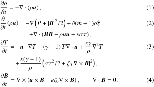 The
pressure, P, satisfies P = ρT, whilst
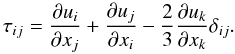
the components of the stress tensor, τ are given by
The
pressure, P, satisfies P = ρT, whilst
the components of the stress tensor, τ are given by
 (5)Note that these
equations have a simple equilibrium solution, corresponding to a hydrostatic polytropic
layer, in which
u = B = 0,
T = 1 + θz and
ρ = Tm.
(5)Note that these
equations have a simple equilibrium solution, corresponding to a hydrostatic polytropic
layer, in which
u = B = 0,
T = 1 + θz and
ρ = Tm.
Non-dimensional parameters.
2.2. Model parameters
Various non-dimensional parameters appear in this model. These are defined in Table 1. Here, γ = 5/3 is
the ratio of the specific heat capacities, m = 1.0 is the polytropic
index, whilst θ = 4.0 is a measure of the thermal stratification. This
choice of parameters implies that the layer is superadiabatically-stratified, with the
temperature varying by a factor of 5 across the layer. The parameter κ is
a non-dimensionalised thermal diffusivity, σ is the Prandtl number,
whilst ζ0 represents the ratio of the magnetic to the thermal
diffusivity at the top of the layer. To interpret these coefficients, it is convenient to
introduce the Reynolds number 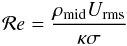 (6)(where
Urms is the rms velocity and
ρmid is the horizontally-averaged mid-layer density) and the
magnetic Reynolds number
(6)(where
Urms is the rms velocity and
ρmid is the horizontally-averaged mid-layer density) and the
magnetic Reynolds number 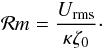 (7)Note that the depth of
the layer, which equals unity in these dimensionless units, has been used as the
characteristic lengthscale in the definitions of these Reynolds numbers. With the
parameter values that are given in Table 1,
ℛe ≈ 420 for the fully-developed hydrodynamic flow, which implies that
the convection is highly turbulent. We have chosen three values for
ζ0, which imply that ℛm ≈ 70
(for ζ0 = 0.2), ℛm ≈ 140
(for ζ0 = 0.1) or ℛm ≈ 280
(for ζ0 = 0.05). Note that the magnetic Prandtl number,
Pm = ℛm/ℛe is
either 0.17, 0.33 or 0.67. As described in the Introduction, Pm ≪ 1
throughout the solar convection zone. Although that parameter regime cannot be reached in
direct numerical simulations, we have at least ensured that
Pm < 1 in all cases. The exploration of the
“low” Pm regime is one of the novel aspects of this study.
(7)Note that the depth of
the layer, which equals unity in these dimensionless units, has been used as the
characteristic lengthscale in the definitions of these Reynolds numbers. With the
parameter values that are given in Table 1,
ℛe ≈ 420 for the fully-developed hydrodynamic flow, which implies that
the convection is highly turbulent. We have chosen three values for
ζ0, which imply that ℛm ≈ 70
(for ζ0 = 0.2), ℛm ≈ 140
(for ζ0 = 0.1) or ℛm ≈ 280
(for ζ0 = 0.05). Note that the magnetic Prandtl number,
Pm = ℛm/ℛe is
either 0.17, 0.33 or 0.67. As described in the Introduction, Pm ≪ 1
throughout the solar convection zone. Although that parameter regime cannot be reached in
direct numerical simulations, we have at least ensured that
Pm < 1 in all cases. The exploration of the
“low” Pm regime is one of the novel aspects of this study.
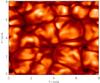 |
Fig. 1 Temperature distribution in a horizontal plane just below the upper surface of the domain, at t = 0. Brighter contours correspond to regions of warmer fluid. |
2.3. Initial conditions
All of the calculations that are considered in this paper are based upon a particular
hydrodynamic flow (as determined by the parameters that are given in Table 1). This is evolved in time until the convection has
reached a statistically-steady state. A snapshot of the resulting flow is shown in
Fig. 1. This plot shows the temperature
distribution in a horizontal plane just below the upper surface of the computational
domain. Bright contours correspond to warm upflows, whilst dark contours correspond to
cooler convective downflows. The flow is characterised by a time-dependent pattern of
granular convection, reminiscent of the one observed at the solar surface. Once the
convection has reached a statistically-steady state, we insert a magnetic field into the
flow. In what follows, we define this insertion time to be t = 0. This
magnetic field takes the form of a weakly twisted, horizontal magnetic flux tube that is
aligned with the y-axis. The radius of the tube, R, is
assumed to be 0.1 (which is 10% of the depth of the domain) in most cases, although a
small number of calculations are carried out with a wider tube (R = 0.15)
. The axis of the flux tube is centred at x = 4.0
and z = 0.75. The three components of this field are given by
![\begin{eqnarray} B_y &=& B_0 \mathrm{e}^{\left[-\left(r/R\right)^2\right]}\\ \nonumber B_x &=& 0.4 (z-0.75)B_y\\ B_z &=& -0.4 (x-4.0)B_y,\nonumber \end{eqnarray}](/articles/aa/full_html/2012/09/aa15747-10/aa15747-10-eq91.png) (8)where
(8)where
 and B0 is a free parameter that can be adjusted to control the
strength of the magnetic field. The factor of 0.4 in the definitions of
Bx and
Bz implies that the initial flux tube is
weakly twisted. The effect of increasing the twist of the tube (by increasing this factor)
is briefly discussed in the next section.
and B0 is a free parameter that can be adjusted to control the
strength of the magnetic field. The factor of 0.4 in the definitions of
Bx and
Bz implies that the initial flux tube is
weakly twisted. The effect of increasing the twist of the tube (by increasing this factor)
is briefly discussed in the next section.
The strength of the magnetic field is a free parameter at this stage. Recalling that we are working with dimensionless variables, it is important to relate the value of B0 to the properties of the flow. We define the plasma β to be the ratio of the gas pressure in the unperturbed polytrope at the initial depth of the tube (i.e. at z = 0.75) to the magnetic pressure. The three cases that are considered in detail in this paper are B0 = 0.96, B0 = 2.53 and B0 = 4.62, which correspond to β = 35, β = 5 and β = 1.5 respectively. It is also of interest to relate the initial magnetic energy density of the field to the kinetic energy density of the convection. At a depth of z = 0.75, a value of B0 = 1.25 would give a peak field strength that would be in approximate equipartition with the kinetic energy of the local convective motions. However, given that the motion is dominated by strong convective downflows, it makes more sense to define an equipartition field strength based upon the mean kinetic energy of the convective downflows at this depth. This implies an equipartition value of Beq = 0.96, which (in turn) implies that the three cases that are considered in detail in this paper correspond to B0 ≈ Beq, B0 ≈ 2.6Beq and B0 ≈ 4.8Beq. In this sense, this range of values for B0 is similar to those considered in previous studies.
Magnetic fields of this strength will exert a dynamically-significant Lorentz force upon
the flow. For a weakly twisted flux tube of this form, the x and
z components of the magnetic field are much smaller than the
By component. As a result of this, the
dominant component of the Lorentz force is due to radial gradients in the magnetic
pressure which tend to force fluid away from the tube axis. To compensate for this
magnetic pressure, we reduce the gas pressure inside the magnetic flux tube at
t = 0 in such a way that the total (gas plus magnetic) pressure
distribution inside the tube matches the gas pressure distribution just before the field
was introduced. Although the tube is not in perfect force balance with its surroundings,
this simple method produces a very good approximation to such a state. Following Cheung et al. (2007) we also modify the local velocity
field within the flux tube so as to minimise convective perturbations to the flux tube
during the early stages of evolution. Using the notation that we adopted for the magnetic
field, we set ![\begin{equation} \vec{u}_{\rm new}=\left(1-\mathrm{e}^{\left[-\left(r/R\right)^2\right]}\right)\vec{u}. \end{equation}](/articles/aa/full_html/2012/09/aa15747-10/aa15747-10-eq111.png) (9)As described in
Cheung et al. (2007), this corresponds to a
velocity field that vanishes along the axis of the tube, smoothly matching up to the
original velocity field near the edge of the tube.
(9)As described in
Cheung et al. (2007), this corresponds to a
velocity field that vanishes along the axis of the tube, smoothly matching up to the
original velocity field near the edge of the tube.
Having specified the gas pressure inside the flux tube, we are free to specify one other
thermodynamic variable. When considering buoyancy instabilities, it is natural to discuss
the entropy of the flux tube. We specify an initial entropy distribution
Snew that is maximal (and uniform) along the tube’s axis,
but matches smoothly onto the background entropy profile, S, at its outer
radius. Hence we set ![\begin{equation} S_{\rm new} = S\left(1-\mathrm{e}^{\left[-\left(r/R\right)^2\right]}\right)+S_{\!0}\,\mathrm{e}^{\left[-\left(r/R\right)^2\right]}. \end{equation}](/articles/aa/full_html/2012/09/aa15747-10/aa15747-10-eq114.png) (10)Normalising the entropy
by Smean(0.75), the horizontally-averaged entropy at
z = 0.75, we consider two different cases. In the lower entropy case,
the peak entropy along the axis of the tube is given by
S0 = 1.26Smean(0.75). This value
of S0 is comparable to the peak entropy in the convective
upflows at this depth. In the higher entropy case, we choose a value for
S0 that is 50% higher than this, i.e.
S0 = 1.9Smean(0.75). Note that
we have also considered some other cases (not shown in this paper) in which the entropy
was uniform in the region r < 0.1. In fact, these
simulations evolved in a very similar way to the radially varying cases. This is
presumably due to the fact that thermal diffusion rapidly smooths out steep gradients in
temperature (which, in turn, smooths out any sharp radial gradients in the entropy
distribution). Given that the evolution of these simulations seems to be rather
insensitive to the precise radial distribution of entropy in the vicinity of the flux
tube, only the radially non-uniform cases will be discussed in this paper.
(10)Normalising the entropy
by Smean(0.75), the horizontally-averaged entropy at
z = 0.75, we consider two different cases. In the lower entropy case,
the peak entropy along the axis of the tube is given by
S0 = 1.26Smean(0.75). This value
of S0 is comparable to the peak entropy in the convective
upflows at this depth. In the higher entropy case, we choose a value for
S0 that is 50% higher than this, i.e.
S0 = 1.9Smean(0.75). Note that
we have also considered some other cases (not shown in this paper) in which the entropy
was uniform in the region r < 0.1. In fact, these
simulations evolved in a very similar way to the radially varying cases. This is
presumably due to the fact that thermal diffusion rapidly smooths out steep gradients in
temperature (which, in turn, smooths out any sharp radial gradients in the entropy
distribution). Given that the evolution of these simulations seems to be rather
insensitive to the precise radial distribution of entropy in the vicinity of the flux
tube, only the radially non-uniform cases will be discussed in this paper.
Summary of the simulations.
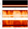 |
Fig. 2 Vertical slices through the x = 4.0 plane, showing contours of By (top), entropy (middle) and the density perturbation (bottom) for the L1 case at t = 0. |
Table 2 summarises the numerical simulations in this study. Most of the simulations (L1–L9) correspond to the lower entropy, thin tube (R = 0.1) cases, for different values of β and different values of ℛm. H1, H2 and H3 illustrate the effects of increasing the initial peak entropy within the thin flux tube (but are otherwise identical to cases L1, L2 and L3). WT1, WT2 and WT3 represent three calculations that were carried out with a wider flux tube, using the lower entropy initial conditions. Finally, in the E1 and E2 simulations, the velocity field, the gas pressure and the entropy distribution are exactly as they were before the field was introduced. Thus, no modification is made to the convection at t = 0. This implies that the Lorentz force will significantly perturb the flow during the early stages of evolution. The rationale for these particular calculations will be discussed later in the paper.
We illustrate the initial condition for one of the low entropy cases (L1) in Fig. 2, which shows the distribution of various quantities in the x = 4.0 plane. The upper plot shows contours of constant By. The localised nature of this initial flux tube is clearly apparent. The middle plot in Fig. 2 shows contours of constant entropy. It is clear from this plot that the peak entropy in the flux tube is comparable to the peak entropy in the convective upflows. We would expect a tube with this entropy distribution to be buoyant relative to its surroundings. Finally, the lower part of Fig. 2 shows the density perturbation in this plane. To obtain this plot, we have subtracted off the polytropic background stratification in order to highlight the variations in ρ due to the magnetic flux tube. As expected, the density perturbation in this strong field (β = 1.5) case takes its minimum value within the flux tube. Here, the minimum value of ρ is approximately 40% of the mean density at this depth. The associated reduction in density is smaller in the β = 5 case, and almost non-existent in the β = 35 case. This simply reflects the fact that the magnetic field is weaker in the higher β cases.
To evolve these simulations, we use a well tested mixed pseudospectral/finite difference code. All horizontal derivatives are evaluated in Fourier space, using standard fast Fourier transform (FFT) libraries. Fourth-order finite differences are used to calculate vertical derivatives. The time-stepping is carried out using a third-order Adams-Bashforth scheme, with a variable time-step. The code is parallelised using MPI. All simulations are carried out on a 512 × 512 × 96 mesh.
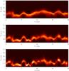 |
Fig. 3 Vertical slices through the x = 4.0 plane, showing contours of By/B0 at t = 0.36 for three different cases, L1 (β = 1.5, top), L2 (β = 5.0, middle) and L3 (β = 35, bottom). In each case, the contours are evenly spaced in the range −0.13 ≤ By/B0 ≤ 0.9. |
3. Results
3.1. Varying the initial conditions
We first consider cases L1, L2 and L3, which correspond to the lower entropy simulations at ℛm ≈ 140, for β = 1.5, β = 5 and β = 35 respectively. In all of these cases, convective motions play a significant role in determining the early evolution of the system, disrupting the flux tube by pulling out loops of magnetic field that are then advected around the domain. The early stages of convective disruption are illustrated in Fig. 3, which shows contours of By/B0 in the x = 4.0 plane for each of these cases at t = 0.36. Normalising the magnetic field by B0 allows us to compare cases with different values of β. Defining the convective turnover time, τconv, to be the inverse of the rms velocity, τconv ≈ 1.56 in these dimensionless units. Hence t = 0.36 corresponds to a small fraction of the turnover time. However, even after this short time period, we see that the flux tube has been perturbed in a significant way by the convective flows. This convective disruption is most apparent in the weaker field (higher β) cases, where small-scale perturbations to the magnetic field have produced a magnetic field with an undulating sea-serpent configuration (as observed in previous calculations, e.g. Cheung et al. 2007). Only in the β = 1.5 case does the field appear to be strong enough to partially resist the convective disruption on this time-scale. Obviously stronger fields possess a higher level of magnetic tension, which makes it more difficult for the surrounding convective motions to perturb the magnetic flux tube.
The subsequent evolution of cases L1 and L3 is illustrated in Fig. 4, which shows the contours of By/B0 in the x = 4.0 plane, for each case, at t = 0.80 and t = 1.59. At these later times, the differences between the stronger field and the weaker field case have become more pronounced. Focusing initially upon the weaker field case (L3), it is clear that the flux tube has been further disrupted by the convective motions. In the t = 0.80 plot, the upflows and downflows in the lower part of the domain have produced many loop-like structures, with several well-defined regions of negative By (which correspond to the dark contours in Fig. 4). Given the relatively weak magnetic fields that are present at this stage of the simulation (even the peak horizontal field strength is now well below the equipartition value that was discussed in the previous section), we would expect the magnetic field to play a relatively passive role in the dynamics. The efficiency with which the convective motions have advected the magnetic flux around the domain would appear to be consistent with this idea. We can see from the t = 1.59 plot for the L3 case that a strong upflow in the vicinity of y = 5 has advected some horizontal magnetic flux into the upper layers of the computational domain. Although convective disruption does also play a role in the stronger field case (L1), there are fewer loop-like structures in the magnetic field distribution at t = 0.80, which suggests that the magnetic flux tube maintains a greater degree of coherence than in the weaker field case. Furthermore, as illustrated in the t = 1.59 plot, a much broader concentration of magnetic flux rises towards the surface regions in this case than it does in the corresponding weaker field calculation. Even though the peak field strength in this emerging flux concentration is a relatively small fraction of its initial value, B0, it is still comparable to the equipartition value, which suggests that it should still exert a dynamically-significant Lorentz force upon the flow. We shall discuss the flux emergence pattern for the L1 case in more detail in the next subsection.
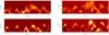 |
Fig. 4 Contours of By/B0 in the x = 4.0 plane. Top: L1 (β = 1.5) at t = 0.80 (left) and t = 1.59 (right). Bottom: the same plots for the L3 (β = 35) case. In the t = 0.80 plots, the contours are evenly spaced in the range −0.25 ≤ By/B0 ≤ 0.45, whilst the contour range is −0.22 ≤ By/B0 ≤ 0.26 in the t = 1.59 plots. |
Figures 3 and 4
clearly show that there is some dependence upon β in these simulations.
The evolution of the flux tube in the weakest field case (L3) appears to be largely
(possibly completely) determined by the surrounding convective motions. However, further
quantitative analysis is needed in order to determine whether or not magnetic buoyancy is
influencing the evolution of the flux tube in the lower β cases. In order
to investigate this possibility, we have traced the evolution of the unsigned emerging
magnetic flux at z = 0. This is given by
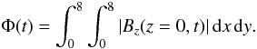 (11)To compare cases
at different values of β, we normalise this quantity by the initial flux
in the y-direction. The results of this quantitative analysis for L1, L2
and L3 are shown in Fig. 5. Cases L2 and L3 both give
very similar flux emergence rates, which indicates that the flux emergence in each case is
driven almost entirely by the convective upflows. The marginal difference between the flux
emergence rates in these two cases would then simply reflect the fact that stronger fields
are more resistant to advection by the convective motions. However, the slightly higher
flux emergence rates in simulation L1 can only be explained if magnetic buoyancy is
enhancing the flux emergence rate in this case. We therefore conclude that magnetic
buoyancy is playing a role in the evolution of the flux tube in this
lower β (stronger field) calculation, helping the convective upflows to
advect dynamically-significant concentrations of magnetic flux into the upper layers of
the domain.
(11)To compare cases
at different values of β, we normalise this quantity by the initial flux
in the y-direction. The results of this quantitative analysis for L1, L2
and L3 are shown in Fig. 5. Cases L2 and L3 both give
very similar flux emergence rates, which indicates that the flux emergence in each case is
driven almost entirely by the convective upflows. The marginal difference between the flux
emergence rates in these two cases would then simply reflect the fact that stronger fields
are more resistant to advection by the convective motions. However, the slightly higher
flux emergence rates in simulation L1 can only be explained if magnetic buoyancy is
enhancing the flux emergence rate in this case. We therefore conclude that magnetic
buoyancy is playing a role in the evolution of the flux tube in this
lower β (stronger field) calculation, helping the convective upflows to
advect dynamically-significant concentrations of magnetic flux into the upper layers of
the domain.
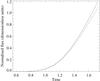 |
Fig. 5 Magnitude of the total unsigned magnetic flux, Φ(t), at z = 0, plotted against time for simulations L1, L2 and L3 (the lower entropy, thin tube, ℛm ≈ 140 cases). The solid line corresponds to L1 (β = 1.5), the dotted line corresponds to L2 (β = 5), whilst the dashed line corresponds to L3 (β = 35). In each case, the flux has been normalised by the initial magnetic flux in the y-direction. |
So far only the strength of the imposed field has been varied. As indicated in Table 2, cases H1, H2 and H3 adopt the same values of β and ℛm as L1, L2 and L3 (respectively), but this time with a higher peak entropy within the initial flux tube. Figure 6 shows the flux emergence as a function of time for these cases. Comparing this plot with Fig. 5, it is clear that there is generally an enhanced rate of flux emergence in these higher entropy calculations. This is to be expected given that the higher entropy flux tube should be more buoyant than those considered in cases L1, L2 and L3. However, it is again notable that there is only a modest dependence upon β in the weaker field cases, H2 and H3, which exhibit very similar flux emergence rates. As in the lower entropy case, there is again a slightly higher rate of flux emergence in the H1 (β = 1.5) case. As before, this suggests that magnetic buoyancy plays a role in the stronger field calculation. We can conclude from this that the enhancement of the flux emergence rate in the stronger field case is a robust result that does not depend critically upon the choice of the initial entropy distribution along the axis of the flux tube. Some simulations with even higher values of the initial entropy were considered. However the emerging flux in these cases tended to be associated with regions of exceptionally high temperature (something that is not observed in the Sun), so these calculations were not pursued in any detail.
 |
Fig. 6 As Fig. 5, but this time for the high entropy cases at ℛm ≈ 140 (H1, H2 and H3). The solid line corresponds to H1 (β = 1.5), the dotted line corresponds to H2 (β = 5), whilst the dashed line corresponds to H3 (β = 35). |
3.2. Varying the flux tube geometry
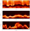 |
Fig. 7 Vertical slices through the x = 4.0 plane for the WT1 simulation, showing the density perturbation (top) and contours of constant By/B0 (middle) at t = 0.36. The lower plot shows contours of constant By/B0 at t = 0.80. In the middle plot, the contours are evenly spaced in the range −0.09 ≤ By/B0 ≤ 0.85. In the lower plot, the corresponding range is −0.06 ≤ By/B0 ≤ 0.55 |
We also considered variations in the twist and the radius of the initial magnetic flux tube. Our aim here was to determine whether it was possible to change the geometry of the tube in such a way as to enhance the effects of magnetic buoyancy. Given that this was the only lower entropy case in which there are any indications of magnetic buoyancy, we used the strong field simulation L1 (β = 1.5) as the basis for investigating these variations in the flux tube geometry. In this case, increasing the original twist by a factor of 10 does not seem to influence the evolution of the tube, or the flux emergence rate. Although this enhancement of the twist does imply that the fieldlines now make approximately 3–4 full turns around the axis of the imposed flux tube, the resulting magnetic tension is still much smaller than the initial magnetic pressure gradient across the radius of the tube. It is therefore not surprising that the dynamics are largely unaffected by this change.
Increasing the width of the flux tube has a much more significant effect upon this system. Case WT1 is identical to L1 in every respect except for the value of R, which has been increased from 0.1 to 0.15. This more than doubles the initial horizontal magnetic flux in the initial condition. The upper two plots in Fig. 7 show the density perturbation and the contours of By/B0 in the x = 4.0 plane at t = 0.36. At this instant in time there is (as in case L1) some indication of modest convective disruption, although there is still a coherent flux tube with a pronounced density deficit. Indeed, at z = 0.75, the minimum density is approximately 60% of the mean density at this depth. So even after the initial phase of evolution, this is still a configuration that should be susceptible to magnetic buoyancy. The lower plot in Fig. 7 shows the distribution of By/B0 in the same plane at t = 0.8. This plot shows that some coherent flux concentrations have risen into the upper layers of the domain. Comparing this plot with the corresponding plot for L1 at t = 0.80 (which is shown in the top left part of Fig. 4), we see that there seems to be more flux in the upper layers of the domain in the wider tube case. To illustrate this point in more quantitative terms, Fig. 8 shows the (unsigned) flux emergence as a function of time for the WT1 simulation, plotted alongside the equivalent flux emergence curve for L1. In each case, the flux is normalised by the initial imposed flux in the y-direction. Given that the (normalised) flux emergence rate is significantly higher in case WT1, we can conclude that magnetic buoyancy is playing a much more significant role in the evolution of this wider magnetic flux tube. This suggests that the efficiency of magnetic buoyancy relative to the effects of convective disruption is determined not only by the initial peak magnetic field strength, but also by the width of the imposed flux tube.
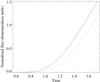 |
Fig. 8 As Fig. 5, but for simulations WT1 and L1. The solid line corresponds to the wide tube case (WT1), whilst the dotted line corresponds to the thin tube case (L1). |
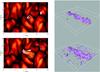 |
Fig. 9 Simulations L1 (top) and WT1 (bottom) at t = 1.59. The plots on the left-hand side show the temperature distribution in a horizontal plane just below the upper surface of the computational domain (shaded contours) and the distribution of Bz in the same horizontal plane (black and white contours). The volume renderings on the right-hand side of this figure show isosurfaces of |B| = 0.25. Some fieldlines have also been traced out along these isosurfaces in order to aid visualisation. |
The left-hand side of Fig. 9 shows the flux emergence patterns for cases L1 and WT1 at t = 1.59. In the L1 case, the vertical magnetic field distribution in the near-surface region is dominated by two well-defined bipolar magnetic regions. As illustrated in Fig. 9, these flux concentrations emerge initially within the warm granular interiors, in regions of convective upflow. However once the magnetic fields reach the near-surface layers, the horizontal convective motions start to sweep these flux concentrations into the intergranular lanes. So at later times these emerging vertical flux concentrations accumulate in the convective downflows. The flux emergence pattern in case WT1 is similar, although more flux has emerged, and the resulting magnetic field distribution is much less localised than the flux emergence pattern from case L1. The volume renderings on the right-hand side of Fig. 9 show isosurfaces of the magnetic field strength (|B| = 0.25). Although the flux tube is wider in the WT1 case, the flux tube structure is similar in both cases. It is clear that the emerging bipoles that are observed at the surface belong to the same undulating flux tube, and are therefore connected by subsurface magnetic field lines. So in each case, the flux tube has resisted convective disruption effectively enough to maintain some semblance of its initial structure throughout the flux emergence process.
3.3. Varying the magnetic Reynolds number
All of the calculations that have been described so far have a magnetic Reynolds number of ℛm ≈ 140. Although the ohmic decay time based on the depth of the layer, τη, is approximately 140 convective turnover times for ℛm ≈ 140, the decay time based upon the width of the flux tube is approximately two orders of magnitude smaller than that. Hence, magnetic dissipation must be playing some role in the evolution of the system on the time-scales of interest. The crucial question is whether or not the evolution of the system is dominated by magnetic dissipation. To investigate this issue, we varied the value of ℛm. Cases L4, L5 and L6 are identical to L1, L2 and L3 in every respect except for the fact that ℛm ≈ 70, as opposed to ℛm ≈ 140. In cases L7, L8 and L9, we adopted a higher value of ℛm ≈ 280. We also carried out some wider tube calculations (WT2 and WT3) with these values for the magnetic Reynolds number. As described in Sect. 2.2, these choices for ℛm ensure that Pm < 1 in all cases, and this restriction upon Pm is the main reason why higher values of ℛm were not considered in the present study.
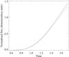 |
Fig. 10 As Fig. 5, but this time for the ℛm ≈ 70 thin tube cases (L4, L5 and L6). The solid line corresponds to L4 (β = 1.5), the dotted line corresponds to L5 (β = 5), whilst the dashed line corresponds to L6 (β = 35). |
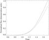 |
Fig. 11 As Fig. 5, but this time for the ℛm ≈ 280 thin tube cases (L7, L8 and L9). The solid line corresponds to L7 (β = 1.5), the dotted line corresponds to L8 (β = 5), whilst the dashed line corresponds to L9 (β = 35). |
Figures 10 and 11 show the normalised flux emergence rates for the thin flux tube, lower entropy cases with ℛm ≈ 70 and ℛm ≈ 280 respectively. These plots should be compared with Fig. 5, which shows the corresponding plot for the ℛm ≈ 140 cases. The first point to notice is that that β dependence of the flux emergence rate is strongly-dependent upon ℛm. In particular, the enhancement of the flux emergence rate due to magnetic buoyancy in the β = 1.5 simulations becomes much more pronounced at higher values of the magnetic Reynolds number. After one convective turnover time (at t ≈ 1.55), the normalised surface fluxes in the ℛm ≈ 70 simulations differ by only a few percent whereas in the ℛm ≈ 280 simulations the normalised fluxes differ by approximately 15% after a similar time period. We can conclude from this that magnetic buoyancy is more efficient at higher magnetic Reynolds number (presumably a consequence of the fact that there is less magnetic dissipation), provided that the magnetic field is strong enough initially to produce a magnetic pressure that is a significant fraction of the local gas pressure. However it is not just the efficiency of magnetic buoyancy that is dependent upon the magnetic Reynolds number. Comparing Figs. 10 and 11, we see that the flux emergence rates in the higher magnetic Reynolds number cases are systematically lower than the corresponding flux emergence rates in the smaller ℛm calculations. Although not shown here, the same is true in the wider tube calculations. The reason for this reduced flux emergence rate is that convective disruption (like magnetic buoyancy) is also more efficient at higher magnetic Reynolds numbers, because there is a greater tendency for magnetic field lines to be advected by the flow. As a result of this, loops of flux are continually removed from the tube, before being reprocessed by the local convective motions. This causes less flux to emerge at the surface of the domain. As described in the Introduction, we know from previous studies (Dorch et al. 2001) that convective motions generally reduce the efficiency of flux emergence. We can now make the stronger statement that this reduction in the flux emergence rate due to convective disruption is more pronounced at higher magnetic Reynolds numbers in the Pm < 1 parameter regime.
Given that the flux emergence rates are strongly dependent upon ℛm, we would also expect the flux emergence patterns to show a similar ℛm-dependence. Figure 12 shows the flux emergence patterns at t = 1.59, alongside a volume rendering of the associated magnetic flux tubes, for cases L7 and WT3 (the lowest β, lower entropy cases for ℛm ≈ 280). Although the strongest emerging flux concentrations are still found in the vicinity of x = 4.0, which corresponds to the location of the axis of the initial magnetic flux tube, many other weaker magnetic flux concentrations are also observed. This indicates that the flux tube has undergone more convective shredding in these higher magnetic Reynolds number cases. This convective disruption is highlighted even more clearly in the volume renderings, particularly in the wide tube case where the magnetic field distribution is highly disordered and fragmented. Although not shown here, very little convective shredding is observed in the ℛm ≈ 70 cases, and the flux emergence pattern is dominated by a small number of coherent dipoles.
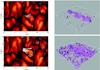 |
Fig. 12 As Fig. 9, but here for the corresponding ℛm ≈ 280, lower entropy cases, L7 (top) and WT3 (bottom). |
3.4. Non-equilibrium expanding flux tubes
In this subsection, we consider the last two cases listed in Table 2, namely E1 and E2. Here, we make no initial perturbation to the flow, pressure or entropy at t = 0. The idea of these simulations is to allow the convection to select its own “initial condition”, by adjusting itself in response to the presence of a dynamically-significant magnetic field. Any magnetic buoyancy is therefore induced in a self-consistent way, albeit from a non-equilibrium initial condition. This approach, whilst clearly oversimplified (and unrealistic for the solar convection zone), has the great advantage that it is not necessary to specify a particular distribution for any of the thermodynamic quantities along the tube, in contrast to the other cases that are considered in this paper. Given that there is considerable uncertainty regarding the most suitable initial conditions for idealised calculations of this type, we would argue that simulations E1 and E2 are useful illustrative calculations in this context.
Obviously, the initial phase of evolution of these simulations is dominated by the effects of the Lorentz force. The radial magnetic pressure gradient tends to drive fluid away from the axis of the tube. Furthermore, this occurs on an Alfvénic time-scale, which means that this process occurs very rapidly (in these cases, the Alfvén speed at the depth of the flux tube is approximately 4 times larger than a typical convective velocity). This pressure-driven radial outflow partially evacuates the flux tube. It also causes the flux tube to expand in the radial direction. By conservation of flux, this expansion leads to a reduction in the mean magnetic field strength within the magnetic flux tube. As a result of this expansion, the flux tube rapidly reaches a state in which it is in (near) total pressure balance with its surroundings. Given that this adjustment is very rapid, convective perturbations play a negligible role during this early phase of evolution.
Having established that these cases rapidly evolve towards pressure-balanced states, we now consider the subsequent evolution of each of these calculations. The initial magnetic field in case E1 is identical to that of case L1, with β = 1.5 and R = 0.1. The top two plots in Fig. 13 show a snapshot of this case at t = 0.36. The upper plot shows the density perturbation in the x = 4.0 plane, whilst the middle plot shows the By distribution in the same plane (normalised by B0). At this instant in time, the minimum density within the flux tube is approximately 75% of the mean density at z = 0.75. Although this level of partial evacuation is not negligible, it is modest compared to some of the other cases. The By/B0 distribution at t = 0.36 is comparable to that shown in the upper plot of Fig. 3 (where the same contour spacings were used). The lower plot in Fig. 13 shows the By/B0 distribution in the x = 4.0 plane at t = 0.8. Again this horizontal magnetic field distribution is comparable to that of the corresponding plot for the L1 case (shown in the top left plot in Fig. 4).
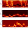 |
Fig. 13 Vertical slices through the x = 4.0 plane for the E1 simulation, showing the density perturbation (top) and contours of constant By/B0 (middle) at t = 0.36. The lower plot shows contours of constant By/B0 at t = 0.80. In the middle plot, the contours are evenly spaced in the range −0.13 ≤ By/B0 ≤ 0.9. In the lower plot, the corresponding range is −0.25 ≤ By/B0 ≤ 0.45. |
In qualitative terms, these plots clearly indicate that the flux tube in this new calculation has evolved in a rather similar way to the flux tube from the L1 case, despite the unrealistic initial conditions. Figure 14 shows the corresponding results for the E2 case (β = 1.5 and R = 0.15), which can be compared directly to WT1 (as illustrated in Fig. 7). At t = 0.36, the minimum density at z = 0.75 for this E2 case is approximately 70% of the mean density at this depth, which is slightly higher than the minimum density at this level at the corresponding stage of the WT1 simulation. However, in almost every other respect, the results from this E2 case are qualitatively rather similar to those of the WT1 simulation. The flux emergence rates for cases E1 and E2 are shown in Fig. 15. These are clearly comparable to the corresponding flux emergence curves for the L1 and WT1 cases. So although the initial conditions in cases E1 and E2 are rather idealised (and probably unrealistic), we have shown that these simulations do evolve in a similar way to our previous calculations. This suggests that local simulations of this type are relatively insensitive to the precise choice of initial conditions, with the evolution of the system (for a given value of ℛm) being determined primarily by the initial magnetic field distribution. Given the wide range of plausible choices of initial conditions in local models of this type, this is an encouraging result.
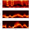 |
Fig. 14 Like Fig. 13, but this time for the E2 simulation. In the middle plot, the contours are evenly spaced in the range −0.09 ≤ By/B0 ≤ 0.85. In the lower plot, the corresponding range is −0.06 ≤ By/B0 ≤ 0.55. |
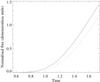 |
Fig. 15 As Fig. 5, but for simulations E1 and E2. The solid line corresponds to the wide tube case (E2), whilst the dotted line corresponds to the thin tube case (E1). |
4. Summary and discussion
We have used numerical simulations to investigate the dynamical evolution of a magnetic flux tube embedded within a granular convective layer. Throughout the calculations we have adopted the same basic hydrodynamic flow, with a Reynolds number of ℛe ≈ 420. When the magnetic flux tube is introduced, the gas pressure is adjusted so that the tube is in pressure balance with its surroundings. The tube is then made buoyant by choosing an appropriate entropy distribution. The subsequent evolution of this tube is influenced by two key processes, namely convective disruption and magnetic buoyancy. However the extent to which magnetic buoyancy plays a role in the flux emergence process depends in a rather subtle way upon the model parameters. In this systematic survey, we varied the initial peak magnetic field strength, the twist and width of the flux tube, the magnitude of the entropy along the tube axis and the magnetic Reynolds number. In all cases, the magnetic Prandtl number, Pm = ℛm/ℛe is less than unity, as would be expected for the solar convection zone. This is the first study of this type to explore this low Pm regime.
At a moderate magnetic Reynolds number of ℛm ≈ 140, the evolution of a thin magnetic flux tube is partially determined by the effects of convective disruption. In the weak field (high β) cases, the magnetic field appears to play a relatively passive role in the dynamics. However, there is an enhanced flux emergence rate in the strongest field cases due to the effects of magnetic buoyancy. Increasing the magnitude of the initial peak entropy along the tube axis does not change the β dependence, but it does increase the rate of flux emergence in all cases. Varying the twist of the flux tube does not seem to influence the evolution of the system (presumably because the magnetic tension is still much weaker than the magnetic pressure gradients in the flux tube). However, increasing the width of the tube does produce an enhanced flux emergence rate in the strong field case. This is presumably because a thicker tube is more robust, and tends to resist convective disruption more effectively than a thinner flux tube. As a result of this, the flux tube maintains its coherence more effectively during the early stages of evolution, which allows magnetic buoyancy to operate in a more efficient manner. So our main conclusion from the ℛm ≈ 140 cases is that the contribution of magnetic buoyancy to the flux emergence process is
directly related not only to the peak field strength, but also to the width of the initial magnetic flux tube.
We also varied the magnetic Reynolds number in this system in order to determine the extent to which the evolution of the tube is influenced by the effects of magnetic dissipation. This parametric survey produced two key results. Firstly, magnetic buoyancy contributes most effectively to the flux emergence process in the low β, high magnetic Reynolds number regime. Secondly, for a given value of β, the flux emergence rate is always lower in the higher ℛm regime. This is due to the fact that convective disruption is much more efficient at higher magnetic Reynolds number (where field lines are more easily advected by the flow). The extent to which this result depends upon the magnetic Prandtl number is unclear, although moving to higher ℛm (thereby increasing Pm) would be computationally simpler than reducing Pm by increasing ℛe. At higher ℛm this convective flow should be capable of sustaining a small-scale dynamo, although it is not clear how such a flow would interact with an emerging flux tube. This is a possible area for future work.
Motivated by some of the uncertainty surrounding the most appropriate choice of initial conditions for problems of this type, we also carried out some idealised simulations in which the gas pressure was not adjusted when the flux tube was introduced. We stress that this is not a realistic situation for the solar convection zone given that this leads to a strong imbalance between the magnetic pressure and the local gas pressure. However, this does allow the system to adjust to the presence of the flux tube in a self-consistent way. This adjustment occurs very rapidly and (somewhat remarkably) the subsequent evolution of the system is comparable to that of the previous set of simulations, at least at comparable magnetic Reynolds numbers. Results from these idealised calculations strongly suggest that the only aspect of the initial conditions that influences the evolution of the flux tube is the initial magnetic field distribution. This is an encouraging result because it suggests that flux emergence simulations are largely insensitive to the precise choice of initial conditions, which is a matter of considerable uncertainty in idealised models of this type.
References
- Abbett, W. P., Fisher, G. H., Fan, Y., & Bercik, D. J. 2004, ApJ, 612, 557 [NASA ADS] [CrossRef] [Google Scholar]
- Archontis, V. 2012, Philos. Trans. Roy. Soc. A, 370, 3088 [Google Scholar]
- Archontis, V., Moreno-Insertis, F., Galsgaard, K., Hood, A., & O’Shea, E. 2004, A&A, 426, 1047 [NASA ADS] [CrossRef] [EDP Sciences] [Google Scholar]
- Bushby, P. J., Houghton, S. M., Proctor, M. R. E., & Weiss, N. O. 2008, MNRAS, 387, 698 [NASA ADS] [CrossRef] [Google Scholar]
- Cheung, M. C. M., Schüssler, M., & Moreno-Insertis, F. 2007, A&A, 467, 703 [NASA ADS] [CrossRef] [EDP Sciences] [Google Scholar]
- Cheung, M. C. M., Rempel, M., Title, A. M., & Schüssler, M. 2010, ApJ, 720, 233 [NASA ADS] [CrossRef] [Google Scholar]
- Dorch, S. B. F., Gudiksen, B. V., Abbett, W. P., & Nordlund, Å. 2001, A&A, 380, 734 [NASA ADS] [CrossRef] [EDP Sciences] [Google Scholar]
- Fan, Y. 2001, ApJ, 554, L111 [NASA ADS] [CrossRef] [Google Scholar]
- Fan, Y., Abbett, W. P., & Fisher, G. H. 2003, ApJ, 582, 1206 [NASA ADS] [CrossRef] [Google Scholar]
- Hood, A. W., Archontis, V., & MacTaggart, D. 2011, Sol. Phys., 157 [Google Scholar]
- Magara, T. 2001, ApJ, 549, 608 [NASA ADS] [CrossRef] [Google Scholar]
- Martínez-Sykora, J., Hansteen, V., & Carlsson, M. 2008, ApJ, 679, 871 [NASA ADS] [CrossRef] [Google Scholar]
- Ossendrijver, M. 2003, A&ARv, 11, 287 [Google Scholar]
- Parker, E. N. 1955, ApJ, 121, 491 [NASA ADS] [CrossRef] [Google Scholar]
- Stein, R. F., Lagerfjärd, A., Nordlund, Å., & Georgobiani, D. 2011, Sol. Phys., 268, 271 [NASA ADS] [CrossRef] [Google Scholar]
- Tortosa-Andreu, A., & Moreno-Insertis, F. 2009, A&A, 507, 949 [NASA ADS] [CrossRef] [EDP Sciences] [Google Scholar]
- Zwaan, C. 1985, Sol. Phys., 100, 397 [NASA ADS] [CrossRef] [Google Scholar]
All Tables
All Figures
|
Fig. 1 Temperature distribution in a horizontal plane just below the upper surface of the domain, at t = 0. Brighter contours correspond to regions of warmer fluid. |
| In the text | |
|
Fig. 2 Vertical slices through the x = 4.0 plane, showing contours of By (top), entropy (middle) and the density perturbation (bottom) for the L1 case at t = 0. |
| In the text | |
|
Fig. 3 Vertical slices through the x = 4.0 plane, showing contours of By/B0 at t = 0.36 for three different cases, L1 (β = 1.5, top), L2 (β = 5.0, middle) and L3 (β = 35, bottom). In each case, the contours are evenly spaced in the range −0.13 ≤ By/B0 ≤ 0.9. |
| In the text | |
|
Fig. 4 Contours of By/B0 in the x = 4.0 plane. Top: L1 (β = 1.5) at t = 0.80 (left) and t = 1.59 (right). Bottom: the same plots for the L3 (β = 35) case. In the t = 0.80 plots, the contours are evenly spaced in the range −0.25 ≤ By/B0 ≤ 0.45, whilst the contour range is −0.22 ≤ By/B0 ≤ 0.26 in the t = 1.59 plots. |
| In the text | |
|
Fig. 5 Magnitude of the total unsigned magnetic flux, Φ(t), at z = 0, plotted against time for simulations L1, L2 and L3 (the lower entropy, thin tube, ℛm ≈ 140 cases). The solid line corresponds to L1 (β = 1.5), the dotted line corresponds to L2 (β = 5), whilst the dashed line corresponds to L3 (β = 35). In each case, the flux has been normalised by the initial magnetic flux in the y-direction. |
| In the text | |
|
Fig. 6 As Fig. 5, but this time for the high entropy cases at ℛm ≈ 140 (H1, H2 and H3). The solid line corresponds to H1 (β = 1.5), the dotted line corresponds to H2 (β = 5), whilst the dashed line corresponds to H3 (β = 35). |
| In the text | |
|
Fig. 7 Vertical slices through the x = 4.0 plane for the WT1 simulation, showing the density perturbation (top) and contours of constant By/B0 (middle) at t = 0.36. The lower plot shows contours of constant By/B0 at t = 0.80. In the middle plot, the contours are evenly spaced in the range −0.09 ≤ By/B0 ≤ 0.85. In the lower plot, the corresponding range is −0.06 ≤ By/B0 ≤ 0.55 |
| In the text | |
|
Fig. 8 As Fig. 5, but for simulations WT1 and L1. The solid line corresponds to the wide tube case (WT1), whilst the dotted line corresponds to the thin tube case (L1). |
| In the text | |
|
Fig. 9 Simulations L1 (top) and WT1 (bottom) at t = 1.59. The plots on the left-hand side show the temperature distribution in a horizontal plane just below the upper surface of the computational domain (shaded contours) and the distribution of Bz in the same horizontal plane (black and white contours). The volume renderings on the right-hand side of this figure show isosurfaces of |B| = 0.25. Some fieldlines have also been traced out along these isosurfaces in order to aid visualisation. |
| In the text | |
|
Fig. 10 As Fig. 5, but this time for the ℛm ≈ 70 thin tube cases (L4, L5 and L6). The solid line corresponds to L4 (β = 1.5), the dotted line corresponds to L5 (β = 5), whilst the dashed line corresponds to L6 (β = 35). |
| In the text | |
|
Fig. 11 As Fig. 5, but this time for the ℛm ≈ 280 thin tube cases (L7, L8 and L9). The solid line corresponds to L7 (β = 1.5), the dotted line corresponds to L8 (β = 5), whilst the dashed line corresponds to L9 (β = 35). |
| In the text | |
|
Fig. 12 As Fig. 9, but here for the corresponding ℛm ≈ 280, lower entropy cases, L7 (top) and WT3 (bottom). |
| In the text | |
|
Fig. 13 Vertical slices through the x = 4.0 plane for the E1 simulation, showing the density perturbation (top) and contours of constant By/B0 (middle) at t = 0.36. The lower plot shows contours of constant By/B0 at t = 0.80. In the middle plot, the contours are evenly spaced in the range −0.13 ≤ By/B0 ≤ 0.9. In the lower plot, the corresponding range is −0.25 ≤ By/B0 ≤ 0.45. |
| In the text | |
|
Fig. 14 Like Fig. 13, but this time for the E2 simulation. In the middle plot, the contours are evenly spaced in the range −0.09 ≤ By/B0 ≤ 0.85. In the lower plot, the corresponding range is −0.06 ≤ By/B0 ≤ 0.55. |
| In the text | |
|
Fig. 15 As Fig. 5, but for simulations E1 and E2. The solid line corresponds to the wide tube case (E2), whilst the dotted line corresponds to the thin tube case (E1). |
| In the text | |
Current usage metrics show cumulative count of Article Views (full-text article views including HTML views, PDF and ePub downloads, according to the available data) and Abstracts Views on Vision4Press platform.
Data correspond to usage on the plateform after 2015. The current usage metrics is available 48-96 hours after online publication and is updated daily on week days.
Initial download of the metrics may take a while.