| Issue |
A&A
Volume 544, August 2012
|
|
|---|---|---|
| Article Number | A2 | |
| Number of page(s) | 10 | |
| Section | Extragalactic astronomy | |
| DOI | https://doi.org/10.1051/0004-6361/201219481 | |
| Published online | 17 July 2012 | |
HS 1700+6416: the first high-redshift unlensed narrow absorption line-QSO showing variable high-velocity outflows
1 INAF – Istituto di Astrofisica Spaziale e Fisica cosmica di Bologna, via Gobetti 101, 40129 Bologna, Italy
e-mail: This email address is being protected from spambots. You need JavaScript enabled to view it.
2 Max-Planck-Institut für extraterrestrische Physik, Giessenbachstrasse, 85748 Garching, Germany
3 Center for Space Science and Technology, University of Maryland, Baltimore County, 1000 Hilltop Circle, Baltimore MD 21155, USA
4 Dipartimento di Astronomia, Universit degli Studi di Bologna, via Ranzani 1, 40127 Bologna, Italy
5 INAF – Osservatorio Astronomico di Bologna, via Ranzani 1, 40127 Bologna, Italy
6 Department of Physics and Astronomy, College of Charleston, Charleston, SC 29424, USA
Received: 25 April 2012
Accepted: 29 May 2012
Abstract
We present a detailed analysis of the X-ray emission of HS 1700+6416, a high-redshift (z = 2.7348) luminous quasar classified as a narrow absorption line (NAL) quasar on the basis of its SDSS spectrum. The source has been observed nine times by Chandra and once by XMM-Newton from 2000 to 2007. Long-term variability is clearly detected between the observations in the 2−10 keV flux, where it varies by a factor of three (~3−9 × 10-14 erg s-1 cm-2), and in the amount of neutral absorption (NH < 1022 cm-2 in 2000 and 2002 and NH = 4.4 ± 1.2 × 1022 cm-2 in 2007). Most interestingly, one broad absorption feature is clearly detected at 10.3 ± 0.7 keV (rest frame) in the 2000 Chandra observation, while two similar features at 8.9 ± 0.4 and at 12.5 ± 0.7 keV are visible when the eight contiguous Chandra observations of 2007 are stacked together. In the XMM-Newton observation of 2002, which is strongly affected by background flares, there is a hint of a similar feature at 8.0 ± 0.3 keV. We interpreted these features as absorption lines from a high-velocity highly ionized (i.e. Fe XXV, FeXXVI) outflowing gas. In this scenario, the outflow velocities inferred are in the range v = 0.12−0.59c. To reproduce the observed features, the gas must have a high column density (NH > 3 × 1023 cm-2), high ionization parameter (log ξ > 3.3 erg cm s-1) and a wide range of velocities (ΔV ~ 104 km s-1). This absorption line quasar is the fourth high-z quasar that displays X-ray signatures of variable high-velocity outflows, and among these, it is the only one that is not lensed. A rough estimate of the minimum kinetic energy carried by the wind of up to 18% Lbol, based on a biconical geometry of the wind, implies that the amount of energy injected into the outflow environment is large enough to produce effective mechanical feedback.
Key words: galaxies: active / galaxies: high-redshift / quasars: absorption lines / quasars: individual: HS 1700+6416 / X-rays: galaxies
© ESO, 2012
1. Introduction
It is now widely accepted that most nearby bulge-dominated galaxies may contain a “relic” super massive black hole (SMBH). The existence of a tight relation between the mass of the SMBH and the properties (mass, luminosity, velocity dispersion) of the host spheroid (Kormendy & Richstone 1995; Silk & Rees 1998; Magorrian et al. 1998; Ferrarese & Merritt 2000) suggest that 1) most bulge galaxies went through a phase of strong nuclear activity during their formation process and 2) the evolution of the galaxy and that of the SMBH must be closely related, implying some sort of interaction or feedback. Models have shown that luminous active galactic nuclei (AGN) might sterilize their host galaxy by heating the interstellar matter through winds, shocks, and ionizing radiation, that strongly inhibits star formation in these galaxies and makes their colors redder (Hopkins et al. 2008; Cattaneo et al. 2009). Some observational evidence for such a scenario is starting to be found in a handful of objects at high redshift (e.g. Cano-Diaz et al. 2012; Page et al. 2012).
Observation log.
One effective way of providing mechanical feedback can be through massive, wide-angle AGN winds or outflows, which can be observed as absorption features in optical/UV/X-ray spectra of AGN. In particular, UV broad absorption lines (BAL, FWHM > 2000 km s-1, Turnshek et al. 1980) of ionized metals are observed in 10 − 15% of optically selected quasi stellar objects (QSOs). Mini-BAL (500 < FWHM < 2000 km s-1, Hall et al. 2002) and narrow absorption line (NAL, FWHM < 500 km s-1, Weymann et al. 1979; Ganguly et al. 2001) QSOs are observed in up to 30% of optically selected QSOs. These absorption features are often strongly blueshifted with respect to the source redshift, indicating outflowing velocities between 103 and few × 104 km s-1 (Ganguly & Brotherton 2008).
In the X-ray band, absorption caused by ionized species such as N VI-VII, O VII-VIII, Mg XI-XII, Al XII-XIII, Si XIII-XVI, as well as L-shell transitions of Fe XVII-XXIV, is observed to be blueshifted by a few 102−103 km s-1 in ~50% of type 1 AGN (the “warm absorber”, e.g. Reynolds 1997; Piconcelli et al. 2005; McKernan et al. 2007). Thanks to the high collecting area of XMM-Newton, Chandra and Suzaku, in the last decade blueshifted absorption lines caused by highly ionized gas (i.e. Fe XXV, Fe XXVI) outflowing at high velocity (vout = 1.5−6 × 10⁴ km s-1) have been observed in several local AGN (Markowitz et al. 2006; Braito et al. 2007; Cappi et al. 2009; Reeves et al. 2009; Tombesi et al. 2010; Giustini et al. 2011).
Finally, X-ray BALs, blueshifted up to vout ~ 2 × 10⁵ km s-1, have been observed in gravitationally lensed BAL QSOs at high redshifts (Chartas et al. 2002; but see also Hasinger et al. 2002; Chartas et al. 2003, 2009; Saez & Chartas 2011). These lines are associated with a zone of circum-nuclear gas, photo-ionized by the central X-ray source, with an ionization parameter1 log ξ ~ 3−5 erg cm s-1 and a column density NH ~ 1022 − 1024 cm-2. These findings suggest the presence of massive clouds of highly ionized absorbing material, outflowing at nearly relativistic velocities from the nuclear regions, which are possibly connected with accretion disk winds and/or the base of a jet (e.g. Ghisellini et al. 2004). However, these features are difficult to observe, because they are intrinsically variable, the gas is highly ionized (and therefore only a few transitions are observable), and the spectral range at which they occur lies at the high-energy edge of the observing band available for present high-throughput X-ray observatories (Cappi et al. 2006).
To understand the physical mechanism responsible for launching and accelerating AGN winds, it is crucial to build up a large sample of sources for which these X-ray features can be studied in detail, especially at high redshift, where the average SMBH accretion rate is higher (Barger et al. 2001). This will allow a deeper understanding of the link between the accretion and ejection processes, quantifying the kinetic energy injected in the environment, and in turn the role of outflows in the formation of cosmic structures. In particular, good quality spectra of high-z QSO that show broad absorption features in the iron K band are limited to three gravitationally lensed BAL and mini-BAL QSOs (APM 08279+5255, PG 1115+080 and H 1413+117, Chartas et al. 2002, 2003, 2007). These sources are the only few optical/UV BAL quasars to date that are bright enough in the X-ray band, mostly due to the strong lensing magnifications, to allow an in-depth spectral analysis.
Here we present a detailed analysis of the X-ray emission of the quasar HS 1700+6416, a high-redshift (z = 2.7348), high-luminosity NAL QSO. HS 1700+6416 is one of the most luminous QSOs in the SDSS (Mi = −30.24) that is not lensed (Reimers et al. 1997). It is not detected in the NVSS radio survey, which has a 5σ sensitivity limit of 2.5 mJy at 1.4 GHz. The source should therefore be considered extremely radio-quiet (log(F1.4 GHz/FR < − 5)2)). HS 1700+6416 is classified as an NAL QSO, shows narrow CII, CIV, SiIII, and Si IV absorption lines in the SDSS spectrum, that are blue-shifted at mildly (~2.4 × 10⁴ km s-1) relativistic velocities (Misawa et al. 2007). The source has a very faint ROSAT counterpart (Reimers et al. 1995).
The paper is organized as follows: Sect. 2 reports on the X-ray observations and data reduction; Sect. 3 presents the spectral analysis, while the main results are discussed in Sect. 4. A standard Λ cold dark matter cosmology with H0 = 70 km s-1 Mpc-1, ΩΛ = 0.73 and ΩM = 0.27 is assumed throughout the paper. Errors are given at 90% confidence level (ΔC = 2.706 for one parameter of interest), unless otherwise specified.
2. X-ray data analysis
2.1. X-ray observations
The quasar HS 1700+6416 lies in a particularly dense and interesting field in the sky. It is close to two clusters, Abell 2246 at z = 0.225 and 2.2′ of angular separation, and V1701+6414 at z = 0.45 and 3.2′ of angular separation (Vikhlinin et al. 1998), and has a foreground overdensity of galaxies and AGN, centered at z = 2.300 ± 0.015 (Digby-North et al. 2010). For this reason, the field has been observed by Chandra and XMM-Newton several times (Table 1), with different scientific goals. In particular, one 50 ks Chandra observation was performed in 2000 to study the cluster V1701+6414 (P.I.: L. Van Speybroeck); one 27 ks XMM-Newton observation in 2002 was performed to study the same cluster (P.I.: F. Jansen), and a series of eight Chandra observations for a total of ~200 ks was taken during nine days in 2007 to study the rate of AGN activity among the galaxies in the overdensity at z = 2.300 (P.I.: K. Nandra).
The 50 ks Chandra spectrum of HS 1700+6416 was presented in Just et al. (2007) in a systematic study of the X-ray properties of the most luminous quasars in the SDSS. The authors applied the Cash statistic to the source unbinned data, and presented the spectra binned at a level of 10 counts per bin, for clearer presentation. They found two consecutive bins in the spectrum of HS 1700+6416 falling ≳ 3σ below a simple power-law model, around 3 keV (11 keV rest frame). The authors claimed the possibility of this being an absorption feature, and reported an improvement of the fit, with the addition of an absorption edge at 2.4 keV (9.0 keV in rest frame), significant at a confidence level > 99.6%.
Misawa et al. 2008 presented an exploratory study of the X-ray properties of NAL-QSOs, analyzing the 50 ks Chandra spectrum and the XMM-Newton spectrum. However, they binned the Chandra spectrum to 20 counts per bin and the XMM-Newton pn and MOS to 150 and 45 counts per bin, respectively, at E > 2 keV. This led to the loss of any information about the presence of absorption features in the spectra. Here we present the re-analysis of these two data sets, with eight additional Chandra observations with exposure times in the range 9 − 32 ks.
2.2. X-ray data reduction
The event files of the Chandra observations were retrieved from the Chandra X-ray Center (CXC) via the Web ChaSeR (Chandra Archive Search and Retrieval) interface. The data reduction was performed following the standard procedures outlined in the Science Analysis Threads for ACIS data at the CIAO (v 4.3) Web site3. The eight repeated observations of 2007 were meant to study the rate of AGN activity in the proto-cluster at z = 2.3, and the quasar HS 1700+6416 was observed only as a by-product. As a result, the source falls close to the ACIS-I ccd gap region in all eight observations (with identical aim point). As a consequence, the effective total exposure at the source position is reduced by ~20% due to dithering.
The XMM-Newton data were retrieved from the XMM-Newton archive4. Standard XMM-Newton SAS tasks epproc and emproc (SAS v. 7.1.0)5 were used to produce calibrated pn and MOS event files. The event files were processed using the latest calibration files and cleaned up from effects of hot pixels and cosmic rays contamination. X-ray events corresponding to patterns 0−12 (0−4) for the MOS(pn) cameras were selected. The XMM-Newton observation was almost completely affected by background flares (see the XMM-Newton User Handbook). We produced a global light-curve at energies > 10 keV, where the contribution from the emission of real X-ray sources is minimized. Different count rate cuts were performed to find the best trade-off between increasing the number of source counts available and decreasing the signal-to-noise ratio. The final cut produced cleaned exposures of ~10 and ~13 ks for pn and MOS, respectively.
We extracted the source counts from circular regions of radius 4′′ for the Chandra pointings. We tried different extraction regions for the XMM-Newton EPIC cameras to minimize the background contribution: 15′′, 25′′ and 40′′, i.e. 70, 80 and 90% of the encircled energy fraction (EEF) respectively. Given the relative flux level of source and background, we chose the smallest extraction region (15′′), which minimized the contribution of the background that could otherwise have strongly affect the spectrum, especially above 2 keV.
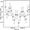 |
Fig. 1 Chandra 0.5 − 8 keV background-subtracted light-curve of HS 1700+6416 extracted from the 50 ks observation of 2000. The bin size is 3000 s. The dashed line shows the mean count rate value of 6.8 × 10⁻³ counts/s. |
The background counts were extracted from annular regions close to the source, avoiding ccd gaps and other sources. The extraction areas were typically ~10 times the source extraction region to average out any position-dependent background features. The obtained spectra have ~400 source net counts in the 0.5 − 8 keV band in the 50 ks Chandra observations, ~310 (300) net counts in the XMM-Newton pn (MOS1 and MOS2 combined), and between 80 − 220 counts in each of the eight repeated Chandra observations.
Given the exposure times of the different observations and the flux level of the source, studying of the short-term variability is feasible only for the long Chandra exposure performed in 2000. Figure 1 shows the 0.5−8 keV background-subtracted light-curve of HS 1700+6416 obtained from the 50 ks Chandra exposure, with a bin size of 3000 s, resulting in > 20 net source counts in each bin. When fitted with a constant, the resulting count rate is 6.8 × 10⁻³ counts s-1, with χ2/d.o.f. = 21.4/16, and a null hypothesis probability P(χ2/ν) = 0.16. Thus, the source is found consistent with being constant on timescales shorter than the duration of the observation (50 ks).
3. Spectral analysis
Below we will describe in detail the spectral analysis performed for the source: first, we determine the properties of the continuum with a simple absorbed power law model; then we focus on the parameters of the strong absorption feature detected in at least two of the four available spectra, using a phenomenological model (a Gaussian absorption line superimposed to the continuum); finally (Sect. 4) we investigate the possibility that the feature might be produced by an absorption edge or by a highly ionized outflowing gas.
Given the low number of source counts available in each observation, and in order to investigate the presence and properties of a possible absorption feature in the X-ray spectra of the NAL QSO HS 1700+6416, we performed all the spectral fits using the Cash statistic (Cash 1979) implemented in Xspec v12. This is a maximum-likelihood function that does not require count binning, which allows one to fully exploit the Chandra and XMM-Newton cameras’ energy resolution. The Cash statistic assumes that the error on the counts is purely Poissonian, and therefore cannot process background-subtracted data. For this reason, a careful characterization of the background spectrum is needed before performing a global fit to the source+background spectrum.
The Chandra global background between 0.5 and 7 keV is complex and was reproduced with two power laws, modified by photoelectric absorption, plus three narrow Gaussian lines to reproduce the features at 1.48, 1.74 and 2.16 keV (Al, Si and Au instrumental lines), plus a thermal (MEKAL) component, to account for the sum of the particle, cosmic, and galactic components of the background (Markevitch et al. 2003; Fiore et al. 2012). The XMM-Newton EPIC pn (MOS) background between 0.5 and 10 keV was reproduced with a similar model, but with two narrow Gaussian lines to account for the prominent features at 1.5 and 8 (1.8) keV (Nevalainen et al. 2005). In each observation the background shape was recovered from background spectra extracted from an extended (8 arcmin) region, excluding the astrophysical sources, in order to collect a large number of counts, thus allowing a detailed, global characterization of the background. Then, each model was rescaled and fitted to the local background, leaving as free parameters the overall normalization and the photoelectric absorption to account for position-dependent variations.
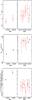 |
Fig. 2 From top to bottom panel: photon index Γ, column density NH and 2 − 10 keV flux in different observations. Time is given in Modified Julian Date. The x-axis scale of the right part of each panel is expanded to show the eight contiguous observations of 2007. |
3.1. Continuum and variability
The source spectra were fitted with a simple power-law, modified by intrinsic neutral absorption at the source redshift, plus galactic absorption (model wabs*zwabs*po in Xspec), fixed to the value measured by Kalberla et al. (2005) at the source coordinates6 (NH,Gal. = 2.3 × 1020 cm-2).
Figure 2 shows the distribution of spectral parameters Γ7, NH8 and the 2 − 10 keV flux, as a function of time (MJD), for all available spectra. The x-axis scale of the right panel of each plot is expanded with respect to the left panel to highlight the results obtained for each of the eight contiguous observations in 2007.
Long-term 2 − 10 keV flux variability by a factor ~3 is clearly detected from ~9 × 10-14 erg s-1 cm-2 in 2002, to ~3.5 × 10⁻¹⁴ erg s-1 cm-2 in 2007. The amount of neutral absorption varied also from NH < 1022 cm-2 in 2000 and 2002 to 4−8 × 1022 cm-2 in 2007. The photon index is constant within the large error bars.
The time span between the eight observations performed in 2007 is 9 days. In this period the spectral parameters of the source appear to be constant, within the error-bars, allowing us to stack all spectra to obtain an average, better quality spectrum. We summed all source and background spectra and produced weighted ARF and RMF with mathpha, addarf and addrmf tools, respectively, which are included in the HEASoft suite9. The matrices were weighted on the basis of the exposure time, but we emphasize that the eight observations have exactly the same aim point, and therefore the different ARFs and RMFs are almost equivalent. As an additional check, we also stacked the eight event files, and extracted a single set of spectra and matrices, from which we obtained consistent results.
HS 1700+6416 also has a rough mass estimate of MBH = 2.5 × 10¹⁰ M⊙ (Shen et al. 2011). We stress that this extreme value, obtained from the C IV emission line, has large uncertainties because there may be a non-virialized (i.e. a disk wind) component in the CIV line (Shen et al. 2008, 2011; Ho et al. 2012). The value therefore should be considered as an upper limit. We can also roughly estimate the BH mass from the 2 − 10 keV luminosity. The 2 − 10 keV intrinsic luminosity of the source decreases from 7.27 × 1045 erg s-1 in 2002 to 3.85 × 1045 erg s-1 in 2007. From the highest value, assuming that the BH is accreting at the Eddington limit, and using a bolometric correction factor of 50 (Vasudevan & Fabian 2007), it is possible to derive a lower limit for the BH mass of 3.9 × 10⁹ M⊙ that, together with the value reported in Shen et al. (2011), gives an indication of the possible BH mass range for the source. Considering the highest available mass estimate, we can derive a Schwarzschild radius (rS = 2GMBH/c2) of ~7.5 × 1015 cm and a light crossing time of ~250 ks in the source frame, which correspond to a variability timescale of ~10 days in the observer frame, while for the lower value of the BH mass, the observed variability timescale is 1.6 days.
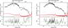 |
Fig. 3 Left panel: observed Chandra 50 ks spectrum and residuals of HS 1700+6416, modeled with a power law modified by Galactic absorption plus intrinsic neutral absorption. The counts are binned to a minimum significant detection of 3σ (and a maximum of 15 counts per bin) only for plotting purposes. Right panel: observed Chandra spectrum and residuals of the source obtained from the eight observations of 2007. The same model and binning strategy as in the left panel are used. The Chandra background is shown in red. |
3.2. Absorption features
Figure 3, left panel, shows the spectrum of HS 1700+6416 obtained from the 50 ks Chandra observation. For plotting purposes only, the spectral counts were binned to yield a minimum of significant detection of 3σ, or 15 channel per bin otherwise. The fit to a simple absorbed power-law model shows significant residuals around ~2.7 keV (observed frame), suggesting the presence of a strong absorption feature. The C-stat value for this simple model is 137.3 for 170 d.o.f. When adding an absorption Gaussian line, with energy, line width, and normalization as free parameters, the resulting C-stat is 117.0 for 167 d.o.f., i.e. a ΔC of 20.3 for three additional parameters (we recall that the change in C-stat from one fit model to the next (ΔC) is distributed approximately as Δχ2 in this range of counts).
Performing an F-test, we found that the addition of an absorption Gaussian line improved the fit at a confidence level > 99.999%. To further assess the statistical significance of this result, extensive (10 000 trials) Monte-Carlo simulations were carried out, producing simulated spectra with the FAKEIT routine in Xspec. The input model is an absorbed power-law with the best-fit parameters obtained from the observed data. The simulated spectra are fitted at first with the simple power-law model, and then adding an absorption Gaussian line, with energy, width, and intensity free to vary (range of Eline = 0.5−7 keV). None of the simulated spectra shows a ΔC = 20 (the higher value being ~15) and therefore we estimate that the probability to detect the observed ΔC by chance is < 1 × 10⁻⁵ (i.e. the feature is significant at confidence level > 99.999%, i.e. > 4σ), confirming the results obtained with the F-test. We emphasize that if the χ2 statistic and count binning (20 counts per bin) are applied, we obtain the following results: chi2/d.o.f. = 44.3/20 for the absorbed power-law model, and chi2/d.o.f. = 17.9/16, when an absorption Gaussian line is added. This turns into a slightly lower significance of 99.6%, in agreement with the value found in Just et al. (2007).
As an additional check we derived the ratio between the observed spectrum of HS 1700+6416 and the observed spectrum of a real featureless source to exclude the possibility that some instrumental effect could be responsible for the broad feature at 2 − 3 keV. We selected the brightest source in the sample of BL Lacs observed in Donato et al. (2003), i.e. PKS 2005-489, with a net count rate of 0.49 count/s, because it has a featureless and flat spectrum and was observed with the same instruments (ACIS-I) and in the same period as the observation of HS 1700+6416. Figure 5 shows the ratio between the two spectra. PKS 2005-489 has a featureless, flat spectrum with Γ = 2.2, i.e. softer than the continuum of HS 1700+6416, as can be seen in Fig. 5 from the steep ratio. More importantly, the feature between 2 and 3 keV is clearly visible in the HS 1700+6416/PKS 2005-489 ratio, confirming that this is not an instrumental feature.
The same analysis as described above was performed for the sum of the eight Chandra observations of 2007. Figure 3 right panel shows the stacked spectrum. The counts were binned in the same way as for the left panel, for plotting purposes. The fit to a simple power law plus neutral absorption model in the 0.5 − 7 keV band shows residuals around 2.4 keV, and a stronger feature at 3.3 keV (observed frame). The C-stat/d.o.f. is 219.9/235 for the simple power-law model, while ΔC are 4.2 and 16.8 for the 2.4 and 3.3. keV features, respectively, for three additional parameters. This results in a confidence level of 81.50% and 99.87%, respectively, when computed with an F-test.
We performed the same type of Monte-Carlo simulations as adopted for the long Chandra exposure, finding that the probability to detect the observed ΔC by chance is 1.03 × 10⁻¹ and 6 × 10⁻⁵, respectively (significance level 89.72% and 9.94%). Accordingly, the detection of the feature at higher energies is significant at >3σ confidence level, while the presence of the feature at lower energies is only marginal (<2σ).
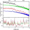 |
Fig. 4 Observed XMM-Newton pn (black) and MOS1+MOS2 (red) spectra and residuals of the source modeled with a power law modified by Galactic absorption plus intrinsic neutral absorption. The pn (MOS) background is shown in green (blue). |
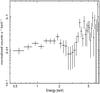 |
Fig. 5 Spectrum of the ratio HS 1700+6416 / PKS 2005-489 for the 50 ks Chandra observation (Cha2000 in Table 2). The spectra were binned to ~200 eV bins. |
Finally, Fig. 4 shows the EPIC pn and MOS spectra extracted from the XMM-Newton observation of 2002. The MOS1 and MOS2 spectra and responses were added with the mathpha, addarf and addrmf tools. As already mentioned, the observation was almost completely affected by background flares, and the cleaned exposure time is ~10 ks. As a consequence, the number of net source counts available in the 0.5−10 keV band is ~300 for each spectrum (pn and combined MOS).
Despite the poor data quality, a hint of an absorption feature around ~2.1 keV can be seen in the residuals of both pn and MOS cameras. In this case the C-stat/d.o.f. is 493.2/529 for the simple power-law model, while ΔC is 14.3 for four additional parameters (line energy, width and two normalizations). This results in a confidence level of 97.50% (F-test). Similar results were obtained with Monte-Carlo simulations (98.15% confidence level). This shows that the evidence of the absorption feature in the XMM-Newton spectra was marginal.
4. Modeling of the absorption features
We tried different models to reproduce the absorption features in the HS 1700+6416 spectra. The results are summarized in Table 2 for the different models and data sets. Model 1 is the simple power-law, modified by intrinsic neutral absorption at the source redshift, plus galactic absorption, discussed above.
Results from spectral fits.
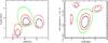 |
Fig. 6 Left panel: 68, 90, 99% confidence contours of Eline vs. the line width from the APL+Gauss model fit of the Chandra 50 ks observation spectrum. The dashed (dotted) contours represent the 68 and 90% confidence contours of the parameters of the two lines in the 2007 stacked Chandra (2002 XMM-Newton) spectrum. Right panel: 68, 90, 99% confidence contours of Eline vs. normalization from the APL+Gauss model fit of the Chandra 50 ks observation spectrum. The dashed (dotted) contours represent the 68 and 90% confidence contours of the parameters of the two lines in the 2007 stacked Chandra (2002 XMM-Newton) spectrum. |
4.1. Gaussian absorption line
Model 2 is the same as model 1 plus one absorption Gaussian line (two for the Chandra 2007 spectrum). Even if this model represents only a phenomenological model to assess the feature significance, the properties of the absorption lines, such as the line centroid energy, the width σ, and the equivalent width (EW hereafter), can be roughly recovered.
The rest frame line centroid energy (Eline) for the 50 ks Chandra spectrum is  keV, the line width
  keV and the equivalent width
  keV (all quantities are given in the rest frame). The left and right panels of Fig. 6 show the 68/90/99% confidence contours of Eline vs. σ and Eline vs. normalization, respectively, for the 50 ks Chandra spectrum (solid curves). Assuming that the absorption feature is coused either by Fe XXV Kα or Fe XXVI Kα, the two strongest absorption lines for a highly ionized gas (Chartas et al. 2009; Saez et al. 2009), with rest frame energies of 6.70 keV and 6.97 keV respectively, we computed the minimum and maximum outflowing velocity, taking the 1σ error on Eline also into account. The resulting velocity is in the range v = 0.30−0.46c.
The observed width of the line in this spectrum is extremely broad. This huge broadening can be due to either high turbulence velocity of the absorbing gas or to the blending of a series of absorption lines, corresponding to different gas shells at different ionization states and/or moving at different velocities (or a combination of the three effects). We underline that although the energy of the Fe XXV Kα and Fe XXVI Kα lines are very close (ΔEline = 0.27 keV), the simple blending of these two lines cannot be responsible for the entire broadening.
The stacked Chandra spectrum of 2007 shows a weak feature at ~2.4 keV and a more prominent one around ~3.3 keV. In the rest-frame, the line parameters are  keV and
  keV, σ1 < 0.95 keV and
  keV,
keV,  keV and
  keV, respectively. The dashed curves in Fig. 6 represent the 68 and 90% confidence contours of the parameters of the two lines in the 2007 stacked Chandra spectrum. The resulting outflowing velocities are in the range v1 = 0.20 − 0.31c and v2 = 0.48 − 0.59c, respectively. Finally, the line parameters for the XMM-Newton pn and MOS spectra fitted together are
  keV, σ < 0.42 keV and
  keV. In this case the resulting outflowing velocity is v = 0.12 − 0.22c. A hint of an emission line, close to the energy of the neutral Fe Kα line, is present both in the Chandra (2007) and in the XMM-Newton spectrum. However, the feature is not statistically significant in either of them, and including this line in the spectral fit did not affect the properties of the absorption feature.
Figure 6 clearly shows that the absorption feature is highly variable in energy, intensity, and width. In particular, if we consider only the two features with the higher significance, i.e. those at 10.3 and 12.5 keV, the probability that the energy of the first absorption line is the same as that of the second is <1 × 10⁻³, i.e. the feature is variable in energy at a confidence level of >99.9%.
4.2. Absorption edge
The third model we assumed to fit the spectral features of HS 1700+6416 was Model 1 modified by an absorption edge. The rest frame edge energy is  keV and the maximum absorption depth is
  for the Chandra spectrum of 2000. For the stacked Chandra spectrum, the two edges have
  and
and  keV, and
  and
and  , respectively. Finally, the edge parameters for the XMM-Newton pn and MOS spectra are
  keV and
  . Given the different shape of the absorption edge with respect to the Gaussian profile, the energies associated to the absorption edges are typically lower than those found for a Gaussian line profile. The rest frame energies were always consistent with K shell ionization thresholds of mildly/highly ionized gas (Fe XVI-FeXXVI) with no blueshifted velocity (Hasinger et al. 2002), except for the highest energy edge of the stacked Chandra spectrum at Eedge2 ~ 11.2 keV, which required an outflowing velocity of at least v/c = 0.18 assuming the recombination energy of hydrogen-like iron, Fe XXVI of 9.28 keV. However, we do not expect to observe single edges in these types of sources, but rather complex absorption structures, caused by the chaotic nature of the gas, which should show a range of ionization parameters and velocities (Ebrero et al. 2011).
4.3. Warm absorber
As another step we used the more physically motivated warm absorber model from XSTAR (Kallman & Bautista 2001) to modify the primary power law. The program computes the spectrum transmitted through a spherical gas shell of constant density, thickness ΔR, at a distance R ≫ ΔR from the ionizing source. In this analysis we used the program implementation that allows one to include the XSTAR output directly within Xspec as a table/model. The input parameters of XSTAR are the gas temperature, density, luminosity, and spectral shape of the ionizing continuum, turbulence velocity, and element abundances, while the output Xspec model, superimposed on the absorbed power-law of Model 1, has three parameters that can be fitted to the spectral data: the ionization parameter ξ, the absorber column density NH, and the absorber redshift (Model 4 in Table 2).
One important input parameter of the warm absorber model is the turbulence velocity of the gas vturb, which controls the broadening of the absorption features. To reproduce the huge width of the absorption feature in the Chandra spectrum of 2000, we had to assume a higher turbulence velocity, vturb = 3 × 10⁴ km s-1. This value is needed to mimic the observed spectral feature but, as said before, it can be interpreted as the result of different (contiguous?) gas shells moving with a wide range of velocities, or, however, as the result of the probably complex dynamics of the wind.
To reproduce the strong feature around the Fe line energies without producing any detectable absorption at lower energies, the absorber must have high column densities (NH > 5.5 × 1023 cm-2) and a very high ionization parameter ( erg cm s-1), such that almost all the Fe atoms are in the form of FeXXV-FeXXVI ions (Kallman et al. 2004), and most of lower-Z elements are completely ionized. In this model, the absorption feature is reproduced by a blend of the Fe XXV and FeXXVI Kα lines. Using the rest frame energies of these lines, i.e. 6.70 and 6.97 keV, respectively, the redshift of the absorber can be translated into a range of outflowing velocity comparable with that obtained from model 2 (v = 0.32 − 0.45c). The improvement of the fit obtained with this model (ΔC ~ 19) is similar to that obtained with the Gaussian absorption line for the same number of free parameters.
The same model was applied to the stacked Chandra spectrum. The data require two highly ionized absorbers, with similar column densities (~3 × 1023 cm-2) and ionization parameters (Log (ξ) > 3.2 erg cm s-1), but outflowing at different velocities, v1 = 0.19 − 0.32c and v2 = 0.47 − 0.58c, to reproduce the features at 2.4 and 3.3 keV, respectively. In this case, the turbulence velocity required to reproduce the width of the lines is slightly lower, 5 × 10³ and 10 × 103 km s-1, respectively. The goodness of fit is again comparable to that obtained for the Gaussian absorption line model. When applied to the XMM spectrum, the model yields a column density NH > 3 × 1023 cm-2, Log ξ > 3.4 and v = 0.12 − 0.20c, with an improvement of the fit of ΔC/Δν = 10.5/3.
4.4. Physical parameters of the gas
Using the values of the column density, ionization parameter, and outflowing velocities derived from the XSTAR model for the different spectra together with the estimated properties of the source, such as BH mass and X-ray (ionizing) and bolometric luminosity, we can give a rough estimate of the location, mass outflow rate, and kinetic energy associated with the wind. We adopted the set of equations collected in Tombesi et al. (2012), that are based on simple assumptions, such as the definition of the ionization parameter and escape velocity for the minimum and maximum distance from the central source.
The minimum radius, computed as the radius at which the outflowing velocity of the wind equals the escape velocity, varies in absolute values within the range 2.5−50 × 1016 cm, assuming the very high (2.5 × 10¹⁰ M⊙) BH mass estimate available from CIV, to 0.4−8.4 × 1016 cm, using the lower limit for the BH mass (3.9 × 10⁹ M⊙), which was estimated assuming an Eddington rate accretion. In both cases (and independently of the BH mass) the very high outflowing velocities measured imply an origin of the wind that is extremely close to the BH, i.e. in the range 3 − 70rs. The maximum radius can be inferred from the definition of the ionization parameter as the maximum distance at which the ionizing luminosity can produce an ionization ξ in a gas with a column density NH: rmax = Lion/ξNH. The ionizing luminosity taken into account by XSTAR when computing the properties of the ionized gas is defined as the unabsorbed luminosity of the source in the range 13.6 eV−13.6 keV. Lion is in the range 0.8 − 6.1 × 1046 ergs s-1, and the associated radius ranges between 0.2−8.9 × 1019 cm, i.e. 2.6 × 10² − 1 × 10⁴rs for a BH mass of 2.5 × 10¹⁰ M⊙, and 1.6 × 10³−7.4 × 10⁴rs for a BH mass of 3.9 × 10⁹ M⊙. The values derived for the Chandra data of 2007 and the XMM data are upper limits, because of the lower limits in ionization parameter. The results obtained for rmax are consistent with what was found in Tombesi et al. (2012) for a sample of lower luminosity local Seyferts, while the higher outflowing velocities observed in HS 1700+6416, with respect to their results, translates into lower values of rmin, i.e. the wind can originate closer to the BH.
To compute the mass outflow rate we used the expression derived by Krongold et al. (2007) for a biconical wind, which was also used in Tombesi et al. (2012), Ṁout = 0.8πmpNHvoutrf(δ,φ). f(δ,φ) depends on the relative orientation of the disk, the wind and the line of sight, but for reasonable angles can be considered of the order of unity. The formula assumes a conical geometry with a constant thickness that is negligible with respect to the distance of the wind from the central source. The minimum mass outflow rates, associated with the minimum radius estimated above, are Ṁout(rmin) = 4 − 6 M⊙/yr, and the associated kinetic energies are in the range ĖK(rmin) = 0.3 − 27 × 1046 erg s-1. These values translate into a minimum Ṁout/Ṁacc = 0.03 − 0.13 and a minimum ĖK/Lbol = 0.01 − 0.18, computed assuming for each observation the Lbol derived from the observed X-ray luminosity, an X-ray bolometric correction of 50, an efficiency η = 0.05, and constant density and velocity. Unfortunately, the maximum mass outflow rates remain unconstrained, because of the combination of lower limits in NH and ξ. However, these high minimum values are already very high, telling us that if they persist and correspond indeed to the simple geometry assumed here, the massive, fast outflowing wind observed in HS 1700+6416 carries a huge amount of energy and is perfectly capable of providing the mechanical power required to produce a significant feedback in the environment, which is estimated to be of about ~5% of the bolometric luminosity (Di Matteo et al. 2005; Ostriker et al. 2010), or even a order of magnitude less in the case of multistage feedback (Hopkins & Elvis 2010). We also underline that the highest values of kinetic energy and mass outflow rate come from the feature with the most secure detection, i.e. from the Chandra spectrum of 2000, which makes our results more robust. Understanding the physics of these winds is necessary to obtain tighter constraints on their properties and on their impact on the surrounding environment.
5. Conclusions
We performed a uniform and comprehensive analysis of all Chandra and XMM-Newton observations taken between 2000 and 2007, and determined the X-ray properties of the high-redshift NAL-QSO HS 1700+6416. The source was found to be constant in flux and spectral parameters on timescales of tens of ks, i.e. the duration of the longest observation available. Furthermore, the X-ray spectral parameters were constant during the eight contiguous observations of 2007, performed in a time interval of 9 days. This allowed stacking the eight spectra taken in 2007, which resulted in a clearer signal-to-noise spectrum for that period. The BH mass estimate available from the SDSS spectrum is extremely high (MBH = 2.5 × 10¹⁰ M⊙) and translates into a variability timescale of ~10 days in the observer frame. Using the bolometric luminosity and Eddington limit accretion, we derived a lower limit for the BH mass of 3.9 × 10⁹ M⊙, implying a variability timescale of ~1.6 days.
On longer timescales, the source is found to be variable on timescales of years, both in the observed 2−10 keV flux, which varies by a factor of 3 between 2002 and 2007, and in the amount of neutral absorption, which is negligible in 2000 and 2002, and becomes about 5 × 1022 cm-2 in 2007.
The most remarkable feature, however, is the detection of a strong, broad and variable absorption feature, observed at energies higher than that of the neutral Fe Kα emission line and up to ~12 keV. The strong, broad absorption feature is clearly detected at high significance (>4σ) in the spectrum extracted from the longest observation available, at an energy of ~10.2 keV. In the stacked spectrum of 2007 a similar feature is detected (>3σ) at higher energies (~12.5 keV). Furthermore, a hint of a feature at ~8−9 keV is observed, albeit at lower significance (~2σ), both in the stacked Chandra spectrum of 2007 and in the short (~10 ks) XMM-Newton spectrum of 2002. Finally, a clear variability is detected in the energy of the line, at least between the two strongest features observed at 10.2 and 12.5 keV (Fig. 6).
In addition to the phenomenological model (a power-law modified by a Gaussian absorption lines) used to determine the significance of the features, we also used a model that included absorption edges instead of Gaussian lines. The energies obtained are consistent with ionization thresholds of mildly/highly ionized gas (Fe XVI-FeXXVI) with no outflowing velocity, except for the highest energy edge of the stacked Chandra spectrum, for which a velocity v ~ 0.2c is required.
Finally, we adopted a more physical approach, modeling the absorption with the XSTAR photo-ionization code. The fit with XSTAR requires for all spectra a dense (NH > 3 × 1023 cm-2) highly ionized (log ξ > 3.2 erg cm s-1) and highly turbulent (vturb = 0.01−0.1c) absorber, so that a blend of Fe XXV and Fe XXVI Kα absorption lines reproduces the spectral feature. The high turbulence velocity is required to reproduce the extreme width of the lines, but this broadening can be interpreted as the result of the superimposition of different gas shells with different velocities, rather than as an internal turbulence. The inferred outflowing velocities are in the range v = 0.12−0.59c.
All these pieces of information make the NAL-QSO HS 1700+6416 the best candidate to be the first unlensed quasar showing X-ray BALs. The measured properties of this source in velocity range, line width, and inferred physical parameters of the obscuring gas are comparable only with those reported for the X-ray BALs APM 08279+5255 and PG 1115+080 (Chartas et al. 2002, 2003). In particular, APM 08279+5255 has a BH mass (MBH ~ 2 × 10¹⁰ M⊙) and an Eddington ratio (LBol/LEdd ~ 0.3) very similar to those of HS 1700+6416. Also similar is the large difference between the outflowing velocities of the X-ray and UV absorption systems, (i.e. a ratio of the order of 10−15), which possibly implies that UV and X-ray BAL are produced by different absorbers at different distances from the central BH.
With the parameters obtained from the fit comprising the ionized absorber, and assumptions on the geometry of the wind and the efficiency of the accretion, we were able to derive a rough estimate of the location of the wind, which spans the range 3−104 rs, and of the minimum mass and kinetic energy content of the wind itself, that varies from few % up to ~13 and ~18% of the mass accretion rate and Bolometric luminosity, respectively. Even if only approximated, these results together with others that emerge from the analysis of local sources and from large blind-search surveys, are starting to quantitatively probe that highly ionized, massive, fast outflowing disk winds can provide the mechanical energy needed to produce the feedback that might be responsible for the well-known relation between galaxy properties and BH masses.
ξ = L/nR2, where L is the ionizing luminosity, n the particle density and R the distance between the ionizing source and the gas (Tarter et al. 1969).
F1.4 GHz is the 1.4 GHz radio flux density.
Defined as F ∝ E − Γ, the power law spectral index.
Defined as M(E) = exp( − Nhσ(E)), the equivalent hydrogen column density of the absorber, where σ(E) is the photo-electric cross-section.
Acknowledgments
We thank the referee for useful comments that improved the paper. The author thanks P. Grandi, E. Torresi and G. G. C. Palumbo for useful discussions. Partial support from the Italian Space Agency (contracts ASI/INAF/I/009/10/0) is acknowledged. This research has made use of the NASA/IPAC Extragalactic Database (NED), which is operated by the Jet Propulsion Laboratory, California Institute of Technology, under contract with the National Aeronautics and Space Administration, and of data obtained from the Chandra Data Archive and software provided by the Chandra X-ray Center (CXC). Also based on observations obtained with XMM-Newton, an ESA science mission with instruments and contributions directly funded by ESA Member States and NASA.
References
- Avni, Y. 1976, ApJ, 210, 642 [NASA ADS] [CrossRef] [Google Scholar]
- Barger, A. J., Cowie, L. L., Bautz, M. W., et al. 2001, AJ, 122, 2177 [NASA ADS] [CrossRef] [Google Scholar]
- Braito, V., Reeves, J. N., Dewangan, G. C., et al. 2007, ApJ, 670, 978 [NASA ADS] [CrossRef] [Google Scholar]
- Cano-Díaz, M., Maiolino, R., Marconi, A., et al. 2012, A&A, 537, L8 [NASA ADS] [CrossRef] [EDP Sciences] [Google Scholar]
- Cappi, M. 2006, Astron. Nachr., 327, 1012 [NASA ADS] [CrossRef] [Google Scholar]
- Cappi, M., Tombesi, F., Bianchi, S., et al. 2009, A&A, 504, 401 [NASA ADS] [CrossRef] [EDP Sciences] [Google Scholar]
- Cash, W. 1979, ApJ, 228, 939 [NASA ADS] [CrossRef] [Google Scholar]
- Cattaneo, A., Faber, S. M., Binney, J., et al. 2009, Nature, 460, 213 [NASA ADS] [CrossRef] [PubMed] [Google Scholar]
- Chartas, G., Brandt, W. N., Gallagher, S. C., & Garmire, G. P. 2002, ApJ, 579, 169 [NASA ADS] [CrossRef] [Google Scholar]
- Chartas, G., Brandt, W. N., & Gallagher, S. C. 2003, ApJ, 595, 85 [NASA ADS] [CrossRef] [Google Scholar]
- Chartas, G., Eracleous, M., Dai, X., Agol, E., & Gallagher, S. 2007, ApJ, 661, 678 [NASA ADS] [CrossRef] [Google Scholar]
- Chartas, G., Charlton, J., Eracleous, M., et al. 2009, New A Rev., 53, 128 [Google Scholar]
- Digby-North, J. A., Nandra, K., Laird, E. S., et al. 2010, MNRAS, 407, 846 [NASA ADS] [CrossRef] [Google Scholar]
- Di Matteo, T., Springel, V., & Hernquist, L. 2005, Nature, 433, 604 [NASA ADS] [CrossRef] [PubMed] [Google Scholar]
- Donato, D., Gliozzi, M., Sambruna, R. M., & Pesce, J. E. 2003, A&A, 407, 503 [NASA ADS] [CrossRef] [EDP Sciences] [Google Scholar]
- Ebrero, J., Kriss, G. A., Kaastra, J. S., et al. 2011, A&A, 534, A40 [NASA ADS] [CrossRef] [EDP Sciences] [Google Scholar]
- Ferrarese, L., & Merritt, D. 2000, ApJ, 539, L9 [NASA ADS] [CrossRef] [Google Scholar]
- Fiore, F., Puccetti, S., Grazian, A., et al. 2012, A&A, 537, A16 [NASA ADS] [CrossRef] [EDP Sciences] [Google Scholar]
- Ganguly, R., & Brotherton, M. S. 2008, ApJ, 672, 102 [NASA ADS] [CrossRef] [Google Scholar]
- Ganguly, R., Bond, N. A., Charlton, J. C., et al. 2001, ApJ, 549, 133 [NASA ADS] [CrossRef] [Google Scholar]
- Ghisellini, G., Haardt, F., & Matt, G. 2004, A&A, 413, 535 [NASA ADS] [CrossRef] [EDP Sciences] [Google Scholar]
- Giustini, M., Cappi, M., Chartas, G., et al. 2011, A&A, 536, A49 [NASA ADS] [CrossRef] [EDP Sciences] [Google Scholar]
- Just, D. W., Brandt, W. N., Shemmer, O., et al. 2007, ApJ, 665, 1004 [Google Scholar]
- Hall, P. B., Anderson, S. F., Strauss, M. A., et al. 2002, ApJS, 141, 267 [NASA ADS] [CrossRef] [Google Scholar]
- Hasinger, G., Schartel, N., & Komossa, S. 2002, ApJ, 573, L77 [NASA ADS] [CrossRef] [Google Scholar]
- Ho, L. C., Goldoni, P., Dong, X.-B., Greene, J. E., & Ponti, G. 2012, ApJ, 754, 11 [NASA ADS] [CrossRef] [Google Scholar]
- Hopkins, P. F., & Elvis, M. 2010, MNRAS, 401, 7 [NASA ADS] [CrossRef] [Google Scholar]
- Hopkins, P. F., Cox, T. J., Kereš, D., & Hernquist, L. 2008, ApJS, 175, 390 [NASA ADS] [CrossRef] [MathSciNet] [Google Scholar]
- Kalberla, P. M. W., Burton, W. B., Hartmann, D., et al. 2005, A&A, 440, 775 [NASA ADS] [CrossRef] [EDP Sciences] [Google Scholar]
- Kallman, T., & Bautista, M. 2001, ApJS, 133, 221 [NASA ADS] [CrossRef] [Google Scholar]
- Kallman, T. R., Palmeri, P., Bautista, M. A., Mendoza, C., & Krolik, J. H. 2004, ApJS, 155, 675 [NASA ADS] [CrossRef] [Google Scholar]
- Kormendy, J., & Richstone, D. 1995, ARA&A, 33, 581 [NASA ADS] [CrossRef] [Google Scholar]
- Krongold, Y., Nicastro, F., Elvis, M., et al. 2007, ApJ, 659, 1022 [NASA ADS] [CrossRef] [Google Scholar]
- Magorrian, J., Tremaine, S., Richstone, D., et al. 1998, AJ, 115, 2285 [NASA ADS] [CrossRef] [Google Scholar]
- Markevitch, M., Bautz, M. W., Biller, B., et al. 2003, ApJ, 583, 70 [NASA ADS] [CrossRef] [Google Scholar]
- Markowitz, A., Reeves, J. N., & Braito, V. 2006, ApJ, 646, 783 [NASA ADS] [CrossRef] [Google Scholar]
- McKernan, B., Yaqoob, T., & Reynolds, C. S. 2007, MNRAS, 379, 1359 [NASA ADS] [CrossRef] [Google Scholar]
- Misawa, T., Charlton, J. C., Eracleous, M., et al. 2007, ApJS, 171, 1 [NASA ADS] [CrossRef] [Google Scholar]
- Misawa, T., Eracleous, M., Chartas, G., & Charlton, J. C. 2008, ApJ, 677, 863 [NASA ADS] [CrossRef] [Google Scholar]
- Nevalainen, J., Markevitch, M., & Lumb, D. 2005, ApJ, 629, 172 [NASA ADS] [CrossRef] [Google Scholar]
- Ostriker, J. P., Choi, E., Ciotti, L., Novak, G. S., & Proga, D. 2010, ApJ, 722, 642 [NASA ADS] [CrossRef] [Google Scholar]
- Page, M. J., Symeonidis, M., Vieira, J. D., et al. 2012, Nature, 485, 213 [NASA ADS] [CrossRef] [Google Scholar]
- Piconcelli, E., Jimenez-Bailón, E., Guainazzi, M., et al. 2005, A&A, 432, 15 [NASA ADS] [CrossRef] [EDP Sciences] [Google Scholar]
- Reeves, J. N., O’Brien, P. T., Braito, V., et al. 2009, ApJ, 701, 493 [NASA ADS] [CrossRef] [Google Scholar]
- Reimers, D., Bade, N., Schartel, N., et al. 1995, A&A, 296, L49 [NASA ADS] [Google Scholar]
- Reimers, D., Kohler, S., Wisotzki, L., et al. 1997, A&A, 327, 890 [NASA ADS] [Google Scholar]
- Reynolds, C. S. 1997, MNRAS, 286, 513 [NASA ADS] [CrossRef] [Google Scholar]
- Saez, C., & Chartas, G. 2011, ApJ, 737, 91 [Google Scholar]
- Saez, C., Chartas, G., & Brandt, W. N. 2009, ApJ, 697, 194 [NASA ADS] [CrossRef] [Google Scholar]
- Shen, Y., Greene, J. E., Strauss, M. A., Richards, G. T., & Schneider, D. P. 2008, ApJ, 680, 169 [NASA ADS] [CrossRef] [Google Scholar]
- Shen, Y., Richards, G. T., Strauss, M. A., et al. 2011, ApJS, 194, 45 [NASA ADS] [CrossRef] [Google Scholar]
- Silk, J., & Rees, M. J. 1998, A&A, 331, L1 [NASA ADS] [Google Scholar]
- Tarter, C. B., Tucker, W. H., & Salpeter, E. E. 1969, ApJ, 156, 943 [NASA ADS] [CrossRef] [Google Scholar]
- Tombesi, F., Cappi, M., Reeves, J. N., et al. 2010, A&A, 521, A57 [NASA ADS] [CrossRef] [EDP Sciences] [Google Scholar]
- Tombesi, F., Cappi, M., Reeves, J. N., & Braito, V. 2012, MNRAS, 422, 1 [Google Scholar]
- Turnshek, D. A., Weymann, R. J., Liebert, J. W., Williams, R. E., & Strittmatter, P. A. 1980, ApJ, 238, 488 [NASA ADS] [CrossRef] [Google Scholar]
- Vasudevan, R. V., & Fabian, A. C. 2007, MNRAS, 381, 1235 [NASA ADS] [CrossRef] [Google Scholar]
- Vikhlinin, A., McNamara, B. R., Forman, W., et al. 1998, ApJ, 502, 558 [NASA ADS] [CrossRef] [Google Scholar]
- Weymann, R. J., Williams, R. E., Peterson, B. M., & Turnshek, D. A. 1979, ApJ, 234, 33 [NASA ADS] [CrossRef] [Google Scholar]
All Tables
All Figures
|
Fig. 1 Chandra 0.5 − 8 keV background-subtracted light-curve of HS 1700+6416 extracted from the 50 ks observation of 2000. The bin size is 3000 s. The dashed line shows the mean count rate value of 6.8 × 10⁻³ counts/s. |
| In the text | |
|
Fig. 2 From top to bottom panel: photon index Γ, column density NH and 2 − 10 keV flux in different observations. Time is given in Modified Julian Date. The x-axis scale of the right part of each panel is expanded to show the eight contiguous observations of 2007. |
| In the text | |
|
Fig. 3 Left panel: observed Chandra 50 ks spectrum and residuals of HS 1700+6416, modeled with a power law modified by Galactic absorption plus intrinsic neutral absorption. The counts are binned to a minimum significant detection of 3σ (and a maximum of 15 counts per bin) only for plotting purposes. Right panel: observed Chandra spectrum and residuals of the source obtained from the eight observations of 2007. The same model and binning strategy as in the left panel are used. The Chandra background is shown in red. |
| In the text | |
|
Fig. 4 Observed XMM-Newton pn (black) and MOS1+MOS2 (red) spectra and residuals of the source modeled with a power law modified by Galactic absorption plus intrinsic neutral absorption. The pn (MOS) background is shown in green (blue). |
| In the text | |
|
Fig. 5 Spectrum of the ratio HS 1700+6416 / PKS 2005-489 for the 50 ks Chandra observation (Cha2000 in Table 2). The spectra were binned to ~200 eV bins. |
| In the text | |
|
Fig. 6 Left panel: 68, 90, 99% confidence contours of Eline vs. the line width from the APL+Gauss model fit of the Chandra 50 ks observation spectrum. The dashed (dotted) contours represent the 68 and 90% confidence contours of the parameters of the two lines in the 2007 stacked Chandra (2002 XMM-Newton) spectrum. Right panel: 68, 90, 99% confidence contours of Eline vs. normalization from the APL+Gauss model fit of the Chandra 50 ks observation spectrum. The dashed (dotted) contours represent the 68 and 90% confidence contours of the parameters of the two lines in the 2007 stacked Chandra (2002 XMM-Newton) spectrum. |
| In the text | |
Current usage metrics show cumulative count of Article Views (full-text article views including HTML views, PDF and ePub downloads, according to the available data) and Abstracts Views on Vision4Press platform.
Data correspond to usage on the plateform after 2015. The current usage metrics is available 48-96 hours after online publication and is updated daily on week days.
Initial download of the metrics may take a while.