| Issue |
A&A
Volume 544, August 2012
|
|
|---|---|---|
| Article Number | A56 | |
| Number of page(s) | 10 | |
| Section | Extragalactic astronomy | |
| DOI | https://doi.org/10.1051/0004-6361/201219410 | |
| Published online | 25 July 2012 | |
Kinetic power of quasars and statistical excess of MOJAVE superluminal motions
1
Instituto de Astrofísica de Canarias,
38200
La Laguna, Tenerife,
Spain
e-mail: This email address is being protected from spambots. You need JavaScript enabled to view it.
2
Departamento de Astrofísica, Universidad de La
Laguna, 38206 La
Laguna, Tenerife,
Spain
3
Dept. d’Astronomia i Astrofísica, Universitat de València,
46100 ,
Burjassot, València,
Spain
Received:
13
April
2012
Accepted:
15
June
2012
Abstract
Aims. The MOJAVE (MOnitoring of Jets in AGN with VLBA Experiments) survey contains 101 quasars with a total of 354 observed radio components that are different from the radio cores, among which 95% move with apparent projected superluminal velocities with respect to the core, and 45% have projected velocities larger than 10c (with a maximum velocity 60c). We try to determine whether this distribution is statistically probable, and we make an independent measure of the kinetic power required in the quasars to produce such powerful ejections.
Methods. Doppler boosting effects are analyzed to determine the statistics of the superluminal motions. We integrate over all possible values of the Lorentz factor, the values of the kinetic energy corresponding to each component. The calculation of the mass in the ejection is carried out by assuming the minimum energy state, i.e., that the magnetic field and particle energy distributions are arranged in the most efficient way to produce the observed synchrotron emission. This kinetic energy is multiplied by the frequency at which the portions of the jet fluid identified as “blobs” are produced. Hence, we estimate the average total power released by the quasars in the form of kinetic energy in the long term on pc-scales.
Results. A selection effect in which both the core and the blobs of the quasar are affected by huge Doppler-boosting enhancement increases the probability of finding a jet ejected within 10 degrees of the line of sight ≳ 40 times above what one would expect for a random distribution of ejection, which explains the ratios of the very high projected velocities given above. The average total kinetic power of each MOJAVE quasar should be very high to obtain this distribution: ~ 7 × 1047 erg/s. This amount is much higher than previous estimates of kinetic power on kpc-scales based on the analysis of cavities in X-ray gas or radio lobes in samples of objects of much lower radio luminosity but similar black hole masses. The kinetic power is a significant portion of the Eddington luminosity, on the order of the bolometric luminosity, and proportional on average to L0.5rad standing for radio luminosity, although this correlation might be induced by Malmquist-like bias.
Key words: quasars: general / galaxies: jets / relativistic processes / methods: statistical / radio continuum: galaxies
© ESO, 2012
1. Introduction
Apparent faster-than-light motion among different components of a quasar, called “superluminal motion”, has been detected for more than 40 years ago (e.g., Gubbay et al. 1969; Knight et al. 1971; Cohen et al. 1971; Whitney et al. 1971). Its measurement has been enhanced with radio observations by the Very Long Baseline Interferometry (VLBI; e.g., Cohen & Unwin 1984), and the latest surveys at the NRAO (National Radio Astronomy Observatory) Very Long Baseline Array (VLBA) conducted to monitor the jet kinematics over several years (Lister et al. 2009a,b). The standard interpretation of these phenomena is that these relativistic jets are observed with a small angle to the line of sight (Rees 1966, see explanation in Sect. 3.1). Narlikar & Chitre (1984) pointed out that the probability of getting the necessary beaming of these events is low. However, a quantitative assesment of this probability should be based on large complete samples. This is one of the pending problems for quasi stellar objects (QSOs), as discussed by López-Corredoira (2011), to which we pay some attention in this paper.
Apart from analyzing the difficulties in understanding this superluminal motion, the calculation of the jet power is also crucial for the understanding of the physical processes taking place in active galaxies. Extragalactic jets represent one of the most powerful events in the Universe, and there is little doubt about their relevant role in the evolution of the host galaxy and its environment (Fabian et al. 2006; McNamara et al. 2005; McNamara & Nulsen 2007). They heat the interstellar and intergalactic media (ISM and IGM, respectively) via shocks (e.g., Zanni et al. 2005; Perucho et al. 2011) and/or mixing (McNamara & Nulsen 2007; De Young 2010, and references therein). The amount of energy deposited depends directly on the jet power and the age of the source (e.g., Merloni & Heinz 2007). Moreover, the jet power is thought to be related to the properties of the host galaxy, such as the mass of the supermassive black hole in its center and the amount of gas in its surroundings (e.g., Merloni & Heinz 2007; Cattaneo et al. 2009). There are, however, still some open problems and challenges regarding these phenomena (see, for instance, the review by Königl 2010).
There are several ways to estimate the kinetic power from observations of AGN jets from scales of parsecs to hundreds of kiloparsecs (see a review in Ghisellini 2011, Sect. 5). Kinetic power can be estimated by means of an analysis of the cavity in X-ray gas, which is assumed to be created by the jet (e.g., Young et al. 2002; Rafferty et al. 2006; Merloni & Heinz 2007). It can also be derived from extended radio emission (e.g., Willott et al. 1999; Punsly 2005; Xu et al. 2009), in terms of the lobe energetics and estimated ages of the radio lobes (e.g., Rawlings & Saunders 1991; Kino & Kawakatu 2005; Ito et al. 2008), assuming that most of the injected energy is converted into work done by the expanding radio source. The time scales used to obtain the kinetic jet power either from the X-ray observations or the extended radio emission on kiloparsec scales, is typically considered on the order of ~ 107 yr (Ma et al. 2008). The results in radio are subject to large errors, such as the determination of the volume and age of the lobes. The age measurement is based on the measured advance velocity of the hot spot, which is assumed to be constant even though numerical simulations have shown that this may not be the case (e.g., Perucho et al. 2011), or on the spectral aging (Punsly 2005), which has been claimed to possibly be inaccurate (Katz-Stone & Rudnick 1997). In all cases, these methods are indirect estimations of the kinetic power, which can be severely underestimated if the kinetic power is dissipated in heating or doing other work than the creation of cavities in the gas.
Estimations of the kinetic power from the jet kinematics have been derived from radio VLBI observations, on the scales of parsecs, and timescales of a few years (e.g., Celotti et al. 1997; Ma et al. 2008; Gu et al. 2009). Celotti et al. (1997) and Gu et al. (2009) analyzed X-ray observations assuming synchrotron self-Compton radiation to be responsible for the X-ray emission. This provided a poor estimation of the kinetic power because of the variability of the sources and the different epochs at which radio and X-ray fluxes were measured (Celotti et al. 1997). Ma et al. (2008) used radio observations to derive the gas density in the jet. Their kinetic power estimations correspond to the energy flux crossing a given section per unit time at the moment in which that jet is observed, and there may be variations in the density of the injected material in the jet (Perucho et al. 2008).
In this paper, we propose something similar but with a totally new method, and we apply it to a recent survey, in which we wish to measure the average total power released by the quasars in the form of kinetic energy in the long term but on pc-scales. Although radio-components represent a fitting artifact without any intrinsic physical meaning, they are generally related to shock waves traveling through the underlying jet flow. In this work, we calculate some properties of these components treating them as physically independent entities, which represents a first-order approximation. In our estimates of the energetics of the radio components, we do not include the internal energy, only the kinetic energy. We derive the mass of the particles from the flux in radio (similar to Ma et al. 2008). The key point of our analysis is that we will directly calculate the kinetic energy by estimating the mass of gas included in each radio component and, hence its kinetic energy rather than a measurement of the energy flux crossing a given section per unit time, and we also include a rough estimate of the frequency of production of these “blobs” in the observations. Our analysis takes advantage of a recent survey of superluminal sources, and we focus only on quasars, in contrast to the BL Lac analysis of Ma et al. (2008). Hence, with this method, we provide a direct calculation of the kinetic energy from observational data rather than analyzing the hypothetical ways in which this energy is dissipated (the creation of cavities in the gas or other features).
Section 2 of our paper describes the data that enables us to perform our statistical analysis. The method of analysis is described in Sect. 3, and the results of its application to the data are given in Sect. 4. Finally, our discussion and conclusions are provided in Sect. 5.
2. Data
Lister et al. (2009a,b) monitored at the frequency of 15 GHz all radio-loud active galactic nuclei (AGNs) whose total flux density in 15 GHz is over 1.5 Jy for declination δ ≥ 0, and over 2.0 Jy for −20° ≤ δ < 0, excluding the zone with Galactic latitude |b| < 2.5°. In total, they observed 135 objects to produce the MOJAVE (MOnitoring of Jets in AGN with VLBA Experiments) survey. Each object was observed for a median of 15 epochs over a period of 13 years (1994−2007). The 15 GHz images have higher than one milliarcsecond resolution, corresponding typically to parsec-scales.
Doppler boosting produces a strong bias in the range of observed angles of the jets, so we
do see neither all AGNs nor all jets. Nonetheless, there is a rough completeness of objects
up to a given total flux density. There may be some missing objects for the adopted flux
density limit, but we assume that the observed objects (135) are more or less complete.
Waldram et al. (2010) gives an independent
measurement of the counts in 15 GHz in an area of 520 deg2,
 Jy-1 sr-1
(valid for a flux F between 5.5 mJy and 1 Jy) or, by integrating
Jy-1 sr-1
(valid for a flux F between 5.5 mJy and 1 Jy) or, by integrating
 (1)If we extrapolate this law
to higher values of F, we find that we should observe around 207 sources in
our area (6.01 sr in the northern cap up to 1.5 Jy; and 2.09 sr in the southern cap up
to 2.0 Jy), which is somewhat higher than the present number of 135, but taking into account
the uncertainties, that we perform an extrapolation, and that some missing sources are
expected in (high extinction) Galactic plane regions, we may assume that completeness is
more or less reasonable.
(1)If we extrapolate this law
to higher values of F, we find that we should observe around 207 sources in
our area (6.01 sr in the northern cap up to 1.5 Jy; and 2.09 sr in the southern cap up
to 2.0 Jy), which is somewhat higher than the present number of 135, but taking into account
the uncertainties, that we perform an extrapolation, and that some missing sources are
expected in (high extinction) Galactic plane regions, we may assume that completeness is
more or less reasonable.
Among the 135 AGNs, a total of 101 objects are quasars with 0.15 < z < 3.40 (roughly half of the sample with z < 1 and half of the sample with z > 1). The classifications of these AGNs were done by Lister et al. (2009a), based on the classification of the optical counterparts, except for four objects that were not classified because they had no optical counterparts. This means that a quasar has broad emission lines in its optical spectrum. This subsample of 101 quasars are the data used in the analysis of this paper. Each object has several components: a main core (containing most of the flux) and other minor components, at least one of which moves with respect to the main core, and has a flux of over 5 mJy. All these motions are relativistic with projected radial linear velocities between 0.2c and 59.1c. In total, the 101 quasars have 101 main cores and 354 ejected blobs, 335 of them are superluminal (projected velocity >c), and 158 of them have projected velocities larger than 10c.
3. Relativistic beaming and its energetic requirements
3.1. Basic kinematic equations
Given a blob expanding from its core with a velocity v, its Lorentz
factor is  (2)with
 The value of Γ is
much larger than one for ultra-relativistic beams. As pointed out by Rees (1966), a superluminal motion of a jet aligned in a
direction very close to the line of sight of the source core may be inferred to have an
“apparent superluminal” projected linear velocity (in units of c:
The value of Γ is
much larger than one for ultra-relativistic beams. As pointed out by Rees (1966), a superluminal motion of a jet aligned in a
direction very close to the line of sight of the source core may be inferred to have an
“apparent superluminal” projected linear velocity (in units of c:
 ), since
 (3)which reaches a
maximum value of
(3)which reaches a
maximum value of  [for θ = sin-1(1/Γ)], a number without
limit, provided that Γ is also unlimited. Figure 1
illustrates the way in which Eq. (3)
behaves. We assume here that the observed apparent velocity of the blobs,
βapp, corresponds to the physical motion of the gas in the
radio component (Lister et al. 2009b), rather than
that of a propagating shock wave. This provides an upper limit to the velocity of the
flow, if those radio components are interpreted as shock waves.
[for θ = sin-1(1/Γ)], a number without
limit, provided that Γ is also unlimited. Figure 1
illustrates the way in which Eq. (3)
behaves. We assume here that the observed apparent velocity of the blobs,
βapp, corresponds to the physical motion of the gas in the
radio component (Lister et al. 2009b), rather than
that of a propagating shock wave. This provides an upper limit to the velocity of the
flow, if those radio components are interpreted as shock waves.
Another property of the relativistic beaming is that the flux of the blob is enhanced by
Doppler boosting. The relationship between the observed flux (F) and the
intrinsic flux if the blob were at rest with respect to the
quasar (F0) is (Ryle & Longair 1967; Narlikar & Chitre 1984; Liu & Zhang 2007)
![Mathematical equation: \begin{equation} F = \frac{F_0}{\left [\Gamma\left (1-\beta \cos \theta \right)\right]^{n_{\rm jet}-\alpha}}, \label{flux} \end{equation}](/articles/aa/full_html/2012/08/aa19410-12/aa19410-12-eq33.png) (4)where
njet = 2 or 3 depending on whether the jet is continuous or
discrete, and α is the spectral index of the blobs with flux
Fν ∝ να.
This also explains why most times we only see the approaching jet and do not see the
receding jet (counter-jet). Figure 2 illustrates the
behavior of this equation for an approaching jet. As can be observed, Doppler factors
smaller than one are also given for high values of θ in an approaching
jet.
(4)where
njet = 2 or 3 depending on whether the jet is continuous or
discrete, and α is the spectral index of the blobs with flux
Fν ∝ να.
This also explains why most times we only see the approaching jet and do not see the
receding jet (counter-jet). Figure 2 illustrates the
behavior of this equation for an approaching jet. As can be observed, Doppler factors
smaller than one are also given for high values of θ in an approaching
jet.
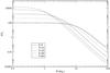 |
Fig. 2 Values of the enhancement of the flux in a blob (Doppler boosting), F/F0, for different values of θ and Γ following Eq. (4), assuming njet − α = 2. |
This relativistic beaming scenario clearly explains the data given by Lister et al. (2009a,b), and indeed Lister et al. (2009b) reproduce their observations using a model with some particular distributions of values of Γ, θ, and F0. We may wonder whether this model is plausible from both a probabilistic and an energetic point of view.
3.2. Probabilistic problem and selection effects
When very few superluminal observed objects were known, one could be surprised to observe the low probability phenomena (Narlikar & Chitre 1984). Now, observations are available for many sources up to a limiting flux density, and we see even more surprisingly that almost all the sources are superluminal, meaning that superluminity is not an anomaly/exception but the rule when observing the brightest blobs.
It is clear from Fig. 1 that, to obtain βapp > 10, as in almost half of the objects in our sample, one needs θ ≲ 10°, and that this is nearly independent of the value of Γ (for θ ≳ 10°, there are very small differences in the value of βapp between the case with Γ = 20 and the case with Γ = 60). The probability of observing by chance an approaching jet with θ ≲ 10° is ~ 0.015; hence, randomly one would expect 5 ± 2 blobs, out of 354, with βapp > 10 for high values of Γ, but we observe 158, which is a totally improbable event by chance. We need to explain an excess in a factor of ~ 30 in the number of sources with θ ≲ 10° with respect to a random distribution. The number of 30 is a minimum ratio because we assumed high values of Γ and there may also be cases of θ ≲ 10° for low Γ. The blobs in each QSO are not independent since they have the same angle ejection, but in all cases the statistics are valid: what we did is equivalent to taking a weighted distribution, with the weight given by the number of its blobs. We could do the statistics directly with the QSOs of average βapp > 10 in the blobs: randomly, one would expect 1.5 ± 1.2 out of 101, and we observe 40, which is nearly the same ratio as before, but ≳ 30 times higher than in a random distribution. If instead the average βapp > 10, we required that the maximum βapp > 10 within a QSO, we would get 60 out of 101 QSOs, which is ≳ 40 times higher than in a random distribution.
We note that this estimation of the excess of probability is independent of the nature of the object, i.e. regardless of whether they are QSOs or other kinds of AGNs. The classification of the same object may change if we see it with different orientations, but our estimation is merely based on the statistics of the probability of a lower jet angle, independently of the kind of AGN.
The explanation stems from the selection effects in a magnitude limited sample: the Malmquist bias, by which we see systematically more luminous quasars at high redshift, but also an effect that leads to higher probabilities of observing low values of θ, that is, accretion discs in the black holes that are nearly face on (Vermeulen & Cohen 1994; Lister & Marscher 1997). This last effect originates from Doppler boosting, the quasars being more luminous for low θ cases (see Fig. 2). Since the limit of detection corresponds to obtaining a total flux (core+blobs) of 1.5/2.0 Jy (respectively, for positive and negative declination), in the cases with a core flux density lower than 1.5/2.0 Jy, we are biased toward a higher number of ejections with low θ.
The Doppler boosting affects both the observed blobs with some superluminal motion with
respect to the core, and core itself. The light we see from the radio core partially
originates from the jet. The flux enhancement in the jet is a factor of around
102−104 for Γ between 5 and 60, and this has a strong effect on
the probability distribution. We assume an intrinsic distribution of quasar fluxes given
by Eq. (1), which only approximately
represents the intrinsic flux of the quasars because it is also affected by Doppler
boosting. Nevertheless, it is adequate for a rough calculation. In addition, we assume
that a fraction ljet of the intrinsic light in the quasar
(including core and blobs) originates from the jet (affected by the Doppler boosting of
Eq. (4)), whereas the remaining
1 − ljet fraction stems from the part of the quasar
intrinsic emission without relativistic motion. The probability distribution for observing
an approaching jet with angle θ is then ![Mathematical equation: \begin{equation} \label{probtheta} P(\theta) = A_P\sin \theta \left[1 - l_{\rm jet} + \frac{l_{\rm jet}}{\left [\Gamma\left(1 - \beta \cos \theta \right)\right]^{n_{\rm jet} - \alpha}}\right]^{1.15}, \end{equation}](/articles/aa/full_html/2012/08/aa19410-12/aa19410-12-eq54.png) (5)where AP
is a normalization constant such that the total probability for all angles is equal to
one. In Fig. 3, we plot the cumulative probability
(5)where AP
is a normalization constant such that the total probability for all angles is equal to
one. In Fig. 3, we plot the cumulative probability
 for
some values of Γ and ljet. As can be observed, a cumulative
probability up to 10 degrees of ≈ 0.5 is obtained with several combinations of
parameters.
for
some values of Γ and ljet. As can be observed, a cumulative
probability up to 10 degrees of ≈ 0.5 is obtained with several combinations of
parameters.

We note that to produce this important enhancement, the observed total density flux
should be dominated by light affected by a Doppler boosting:
![Mathematical equation: \hbox{$\frac{l_{\rm jet}}{\left [\Gamma\left (1-\beta \cos \theta \right)\right]^{n_{\rm jet}-\alpha }}\gg 1-l_{\rm jet}$}](/articles/aa/full_html/2012/08/aa19410-12/aa19410-12-eq60.png) . This would not be
possible if we assumed that the core light is unboosted, because in most sources, most of
the observed flux comes from the core. However, this assumption of unboosted core light is
incorrect because the radio flux we observe in the core originates mainly from the jet.
Bell (2012) claimed that Doppler boosting cannot
precisely explain these large ratios of superluminal motions because the core light is
unboosted, but we doubt the validity of Bell’s statement. Nevertheless, we refer the
reader to the interesting discussion of Bell (2012).
. This would not be
possible if we assumed that the core light is unboosted, because in most sources, most of
the observed flux comes from the core. However, this assumption of unboosted core light is
incorrect because the radio flux we observe in the core originates mainly from the jet.
Bell (2012) claimed that Doppler boosting cannot
precisely explain these large ratios of superluminal motions because the core light is
unboosted, but we doubt the validity of Bell’s statement. Nevertheless, we refer the
reader to the interesting discussion of Bell (2012).
3.3. Estimate of the mass of the gas in the component
The total mass embedded in the ejected blob can be calculated under the assumption that
all its particles produce synchrotron radiation (i.e. there is no thermal component) and
the assumption of minimum energy, which states that the magnetic field and particle energy
distributions are arranged in the most efficient way to produce the observed synchrotron
emission. This approach thus provides a lower limit to the number of particles (and,
therefore, of the mass) in the considered region. The radio luminosity of each blob is
associated with its mass through (Perucho & Martí 2002) ![Mathematical equation: \begin{eqnarray} \label{masa_j} && M_j = \frac{L_{{\rm radio},j}C_1m_{\rm e}}{C_3B_{\min}f_{\rm synch}}\frac{2 + 2\alpha }{2\alpha } \frac{\nu _{\max}^\alpha - \nu _{\min}^\alpha }{\nu _{\max}^{(1+\alpha)} -\nu _{\min}^{(1+\alpha)}}, \\[1.5mm] \label{bmin} && B_{\min} = \left(\frac{6\pi AL_{{\rm radio},j}}{V_j}\right)^{2/7}, \\[1.5mm] \label{A_masa_j} && A = \frac{\sqrt{C_1}}{C_3}\frac{2+2\alpha }{1+2\alpha} \frac{\nu_{\max}^{(1/2+\alpha)} - \nu_{\min}^{(1/2+\alpha)}}{\nu _{\max}^{(1+\alpha)} -\nu _{\min}^{(1+\alpha)}}, \end{eqnarray}](/articles/aa/full_html/2012/08/aa19410-12/aa19410-12-eq61.png) where
C1 = 6.3 × 10¹⁸ [cgs],
C3 = 2.4 × 10⁻³ [cgs],
νmin = 107 Hz, and
νmax = 1011 Hz. The
factor fsynch is the ratio of the mass producing significant
synchrotron emission, that is, the collective mass of the electrons or positrons (with
mass me = 9.11 × 10⁻²⁸ g), with respect to the
total mass including also the protons. Protons do have a much lower emissivity, which can
be assumed to be negligible. Vj is the
physical volume of the blob, which we take as the volume of an ellipsoid
where
C1 = 6.3 × 10¹⁸ [cgs],
C3 = 2.4 × 10⁻³ [cgs],
νmin = 107 Hz, and
νmax = 1011 Hz. The
factor fsynch is the ratio of the mass producing significant
synchrotron emission, that is, the collective mass of the electrons or positrons (with
mass me = 9.11 × 10⁻²⁸ g), with respect to the
total mass including also the protons. Protons do have a much lower emissivity, which can
be assumed to be negligible. Vj is the
physical volume of the blob, which we take as the volume of an ellipsoid
 (9)where aj
is the half width half maximum (FWHM/2) of the physical size (that is,
multiplying the angular size by the angular cosmological distance),
and rj is the axial ratio of the Gaussian
ellipsoidal fit to the blob structure given by Lister et al. (2009b). The last factor is the correction of the projection of the
ellipsoid and its relativistic contraction, assuming that the jet is a moving
bar/ellipsoid (Ghisellini 2000, Sect. 5.1). For the
projected direction of the jet cross-section, we assume that the axis is equal to the one
perpendicular to the direction of the jet propagation (i.e., we assume a cylindrical
component). The volume used in the calculations is that obtained from the average value
for all epochs.
(9)where aj
is the half width half maximum (FWHM/2) of the physical size (that is,
multiplying the angular size by the angular cosmological distance),
and rj is the axial ratio of the Gaussian
ellipsoidal fit to the blob structure given by Lister et al. (2009b). The last factor is the correction of the projection of the
ellipsoid and its relativistic contraction, assuming that the jet is a moving
bar/ellipsoid (Ghisellini 2000, Sect. 5.1). For the
projected direction of the jet cross-section, we assume that the axis is equal to the one
perpendicular to the direction of the jet propagation (i.e., we assume a cylindrical
component). The volume used in the calculations is that obtained from the average value
for all epochs.
The factor α is the spectral index, and
Lradio,j is the total radio luminosity
 (10)where
dL(z) is the luminosity
distance of the quasar at redshift z (assuming a standard cosmology with
h = 0.7, Ωm = 0.3, and ΩΛ = 0.7) and
Fradio/rest,j the total
flux at rest with respect to the quasar (that is, corrected for Doppler boosting),
observed between νmin and νmax.
Using Eq. (4) and integrating the total
density flux over the range of frequencies, we get
(10)where
dL(z) is the luminosity
distance of the quasar at redshift z (assuming a standard cosmology with
h = 0.7, Ωm = 0.3, and ΩΛ = 0.7) and
Fradio/rest,j the total
flux at rest with respect to the quasar (that is, corrected for Doppler boosting),
observed between νmin and νmax.
Using Eq. (4) and integrating the total
density flux over the range of frequencies, we get ![Mathematical equation: \begin{eqnarray} \label{fluxradio} F_{{\rm radio/rest},j} &= \frac{F_j}{\nu _0^\alpha (1+\alpha)} \left[\nu_{\max}^{(1+\alpha)} - \nu_{\min}^{(1+\alpha)}\right] \nonumber\\[1.5mm] &\quad \times \left[\Gamma_j\left(1-\beta _j\cos \theta _j\right)\right]^{n_{\rm jet}-\alpha}, \end{eqnarray}](/articles/aa/full_html/2012/08/aa19410-12/aa19410-12-eq82.png) (11)where
Fj is the observed density flux at
frequency ν0 = 15 GHz of the blob (we take the average of all
epochs evaluated by Lister et al. 2009b),
and θj obtained
from βapp,j
and Γj through the relationship of Eq. (3):
(11)where
Fj is the observed density flux at
frequency ν0 = 15 GHz of the blob (we take the average of all
epochs evaluated by Lister et al. 2009b),
and θj obtained
from βapp,j
and Γj through the relationship of Eq. (3):  (12)There are two solutions
to
θj(βapp,j,Γj),
respectively, for the “+” and “–” sign in this equation. They correspond to the two values
of θ for a given βapp and Γ that are
observed in Fig. 1.
(12)There are two solutions
to
θj(βapp,j,Γj),
respectively, for the “+” and “–” sign in this equation. They correspond to the two values
of θ for a given βapp and Γ that are
observed in Fig. 1.
In Eqs. (6), (8), and (11), there are values of α for which there is some
zero in both the numerator and the denominator, but there is no divergence in the limit.
For instance, for Eq. (6),
 .
.
3.4. Kinetic energy of the observed blobs
We do not know the value of Γ for each blob, so we have to integrate over all of its
possible values. The kinetic energy of all the “observed” components in a quasar is
(herein, we refer to as “kinetic” the total energy excluding the energy associated with
the released mass at rest, that is
E = Mc2(Γ − 1))
 (13)where
![Mathematical equation: \begin{eqnarray} \langle f\rangle &\equiv \sum_{j=1}^N\int_{\sqrt{1 + \beta_{{\rm app},j}^2}}^{\Gamma_{\max}}{\rm d}\Gamma _j \nonumber\\[1.5mm] &\quad \times \left[P_1\left(\Gamma_j \big|\beta_{{\rm app},j}\right) \sum_{\theta _j=+,-}P_2\left(\theta _j,\Gamma _j\right)f_j\left(\Gamma _j,\theta _j\right)\right], \end{eqnarray}](/articles/aa/full_html/2012/08/aa19410-12/aa19410-12-eq93.png) (14)and
j stands for the number of components from 1 to N,
and Mj, Γj are
their respective masses at rest and Lorentz factors. The probability of having a value of
the Lorentz factor equal to Γj provided that the apparent
projected velocity in units of c
is βapp,j, is (Bayes’ theorem)
(14)and
j stands for the number of components from 1 to N,
and Mj, Γj are
their respective masses at rest and Lorentz factors. The probability of having a value of
the Lorentz factor equal to Γj provided that the apparent
projected velocity in units of c
is βapp,j, is (Bayes’ theorem)
 (15)where
CP is a constant of normalization of the
probability over the range between
(15)where
CP is a constant of normalization of the
probability over the range between  (minimum value of Γ) and Γmax. We take the Lorentz factor distribution from Liu
& Zhang (2007), which was derived precisely
with MOJAVE data as well, with
P(Γ) ∝ ΓaΓ and
aΓ = −1.73. The last factor stems from the probability of
beaming in this range; that is, an amount proportional to the range of
values θj that make
βapp ≥ βapp,observed.
It is (Narlikar & Chitre 1984, Eq. (8))
(minimum value of Γ) and Γmax. We take the Lorentz factor distribution from Liu
& Zhang (2007), which was derived precisely
with MOJAVE data as well, with
P(Γ) ∝ ΓaΓ and
aΓ = −1.73. The last factor stems from the probability of
beaming in this range; that is, an amount proportional to the range of
values θj that make
βapp ≥ βapp,observed.
It is (Narlikar & Chitre 1984, Eq. (8))
 (16)In Fig. 4, we plot an example of the probability distribution for
βapp = 6.74.
(16)In Fig. 4, we plot an example of the probability distribution for
βapp = 6.74.
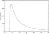 |
Fig. 4 Probability distribution of the Lorentz factor for a jet with an observed projected linear velocity (in units of c) of βapp = 6.74, as in the case of QSO 0016+731. |
The sum
“ ∑ θj = + ,−”
stands for the sum over the two possible values of
θ(Γj,βapp,j)
given in Eq. (12) with the respective
probabilities ![Mathematical equation: \begin{eqnarray} P_2\left(\theta _j, \Gamma_j\right) &= C_{P2}\left(\Gamma_j\right)\int _0^{\theta_j}{\rm d}\theta \sin \theta \nonumber\\[1.5mm] & = C_{P2}\left(\Gamma_j\right) \left(1-\cos \theta_j\right), \end{eqnarray}](/articles/aa/full_html/2012/08/aa19410-12/aa19410-12-eq109.png) (17)where CP2
is a constant of normalization such that the sum of the two probabilities with sign +
and − in Eq. (12) equals one.
(17)where CP2
is a constant of normalization such that the sum of the two probabilities with sign +
and − in Eq. (12) equals one.
3.5. Total kinetic power
To calculate the total power released, we must multiply each energy contribution by its
frequency. We note that the sample was observed over a period of 13 years. We assume
statistically that the average radial position during the period of the
components (Rj) is in the middle of the
observable range, i.e., the range in which the jet might be observed to have sufficient
flux density to be detected. We neglect that components get brighter or fainter during
this period. While the sources in the sample are moving with an average angular
speed μj (we neglect the acceleration), the
order of magnitude of the frequency for each of the considered (or studied) events is
 (18)The
(1 + zj) factors stem from the time
dilation caused by the cosmological expansion. Including the frequency of events, the
power released in the form of kinetic energy is the kinetic energy of Eq. (13) multiplied by the frequency
(18)The
(1 + zj) factors stem from the time
dilation caused by the cosmological expansion. Including the frequency of events, the
power released in the form of kinetic energy is the kinetic energy of Eq. (13) multiplied by the frequency  (19)The factor two
accounts for the counter-jet. This counter-jet was not observed in any of the 101 quasars
of our sample, which indicates that the viewing angles of all of them are small.
(19)The factor two
accounts for the counter-jet. This counter-jet was not observed in any of the 101 quasars
of our sample, which indicates that the viewing angles of all of them are small.
We cannot see the ejections for low value of Γj because they have not undergone sufficient Doppler boosting to make them observable; to correct for this, one should divide this power by a factor of P3 calculated as described in Appendix A. Furthermore, the jets are ejected in cones with very small intrinsic opening angles (Pushkarev et al. 2009, with MOJAVE data), so we can assume that the correction for the unobserved blobs, required owing to the lower Doppler boosting in a cone, is negligible. If the emission cones were wider, a correction should be introduced, as explained in Appendix B. In this paper, we include the correction of the factors 1/P3 (derived in Appendix A) for each energy, but we neglect the factors 1/P4 (derived in Appendix B).
3.6. Parameters used for our calculations
For the calculation of the kinetic energy/power, we need the parameters provided by Lister et al. (2009a,b) for each quasar and each component.
The value of α, the spectral index, should be close to zero, since most of the components have a flat radio spectrum (Lister & Marscher 1997; Lister et al. 2009b). It is a rough extrapolation to assume that this spectral index is valid for the range between 107 and 1011 Hz, since we do not have information for the whole range and we know that these components are not optically thick in the whole range. This flat spectrum is most likely a combination of intrinsic emission and self-absorption. Nonetheless, as we show in Sect. 4.2, a different choice of α would not give significantly lower values of the kinetic power.
The jet is considered continuous, so njet = 2 (Lister & Marscher 1997; Lister et al. 2009b). The value of minimum flux density for the detection of a blob is, as we have said, Fmin = 5 mJy. For the maximum allowed value of the Lorentz factor, we take Γmax = 60, given that the maximum observed value of βapp is around that value.
A critical parameter is the fraction of emitting particles, which requires knowledge of
the composition of the plasma in the blob. This is composed of electron-positron pairs and
electron-proton pairs. There have been several analyses indicating that the number of
electrons is ≲ 10 times the number of protons in the jet (Kataoka et al. 2008; Ghisellini & Tavecchio 2010, and references therein). A blob composed only of
electron-positron pairs would decelerate strongly and not allow superluminal motion to
occur (Ghisellini & Tavecchio 2010), owing
to both a loss of energy in an inverse Compton process and the lower mass/unit charge that
would give a lower inertia to the jet. Assuming the minimum possible number of protons
(which contribute to a minimum kinetic energy), we take the number of 10 electrons per
proton, hence the ratio of the mass of particles producing significant synchrotron
emission to the total mass is  .
.
4. Results
We apply the aforementioned calculation to the quasar QSO 0016+731 (the first one in the list) at redshift z = 1.781. It has only one observed jet with ⟨ F1 ⟩ = 144 mJy, ⟨ R1 ⟩ = 1100 μas, μ1 = 87 μas/yr, βapp,1 = 6.74, a1 = 330 μas, and r1 = 1.00. This gives a distribution of Lorentz factors similar to those given in Fig. 4 and an average value of ⟨ Γ1 ⟩ = 20.8, and the average angle with the line of sight ⟨ θ1 ⟩ = 15°. The average values within this distribution are EK,obs. = 4.33 × 1055 erg = 24 M⊙c2, ⟨ M1 ⟩ = 0.75 M⊙, volume of V1 = 77 pc3, and EK,total = 1.03 × 1056 erg. That is, the observed blob has a mass of around three quarters of a solar mass and a kinetic energy of around 24 M⊙c2, whereas the total released energy is 2.4 times higher including the jets that we do not see. The frequency of an event such as this is estimated to be freq1 ~ 0.073 yr-1 and consequently pK,total ~ 2 × 1047 erg/s.
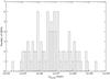 |
Fig. 5 Histogram of the distribution of kinetic power derived with Eq. (19) for the 101 quasars of the MOJAVE complete sample (Lister et al. 2009a,b). |
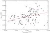 |
Fig. 6 Kinetic power released in jets versus the radio luminosity of the parent quasar. The solid line is the fit indicated in the text. |
One might think that the QSO 0016+731 is a statistically anomalous case in which we have
observed far more superluminal jets than on average expected. To avoid this suspicion, we do
the same calculation for the rest of the 101 quasars. The histogram of Fig. 5 shows the distribution of the minimum values
of pK,total. As can be observed, the case of
QSO 0016+731 with
pK,total ~ 2 × 1047 erg/s is quite
normal, and is quite close to the median value. There is large dispersion of values up to
pK,total ~ 3 × 1049 erg/s, which
is reached for QSO 2037+511 at z = 1.686 with one observed blob, and
βapp,1 = 3.3. The average power and jet angle
of the whole sample are ![Mathematical equation: \begin{eqnarray} && \overline{p_{\rm K,total}} = (7.5\pm 2.9)\times 10^{47}~{\rm erg/s}, \\[1.5mm] && \overline{\theta} = (12.1\pm 1.4)~{\rm deg}. \end{eqnarray}](/articles/aa/full_html/2012/08/aa19410-12/aa19410-12-eq149.png)
4.1. Correlation of kinetic power with the luminosity of the quasar
In Fig. 6, one can see the dependence of the kinetic
power on the radio luminosity for the
quasar Lradio/rest,QSO,
where we have considered the average 15 GHz flux of the core and we applied Eq. (11) with αQSO = 0
but without the Doppler boosting correction (Γ = 1, β = 0). There is a
significant correlation in this figure of  (significant at 3.5-σ), where
x ≡ log 10Lradio/rest,QSO
(erg/s), and
y ≡ log 10PK,total (erg/s).
However, there is also strong correlation both between x and redshift and
between y and redshift (the range is
0.15 < z < 3.40), as
expected due to the Malmquist bias, so this correlation mostly means that the most distant
objects have the highest luminosities and highest kinetic powers. If we assumed that there
is no evolution (i.e., there is no dependence of quasar luminosities and kinetic powers on
redshift), we could interpret the correlation of Fig. 6 as something inherent to the characteristics of the quasars. The best
power-law fit
(significant at 3.5-σ), where
x ≡ log 10Lradio/rest,QSO
(erg/s), and
y ≡ log 10PK,total (erg/s).
However, there is also strong correlation both between x and redshift and
between y and redshift (the range is
0.15 < z < 3.40), as
expected due to the Malmquist bias, so this correlation mostly means that the most distant
objects have the highest luminosities and highest kinetic powers. If we assumed that there
is no evolution (i.e., there is no dependence of quasar luminosities and kinetic powers on
redshift), we could interpret the correlation of Fig. 6 as something inherent to the characteristics of the quasars. The best
power-law fit 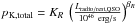 gives
KR = (5.0 ± 1.1) × 1046 erg/s, and
βR = 0.47 ± 0.13, which might be
interpreted as the relationship under the assumption of non-evolution.
gives
KR = (5.0 ± 1.1) × 1046 erg/s, and
βR = 0.47 ± 0.13, which might be
interpreted as the relationship under the assumption of non-evolution.
The dependence on the mass of the black hole can be evaluated in some cases in which the
virial mass of the black hole is calculated. There are 24 QSOs in common with the sample
of the Sloan Digital Sky Survey in the Data Release 7 (SDSS-DR7; Schneider et al. 2010), and in which the black hole virial masses were
calculated (Shen et al. 2011). We take their
fiducial values and compare with our kinetic power in the 24 QSOs in common in Fig. 7. There is a slight correlation in this figure of
 (significant at 1.9-σ), where
x ≡ log 10MBH(M⊙),
y ≡ log 10PK,total (erg/s),
which we consider not significant enough to take further conclusions.
(significant at 1.9-σ), where
x ≡ log 10MBH(M⊙),
y ≡ log 10PK,total (erg/s),
which we consider not significant enough to take further conclusions.
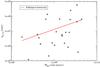 |
Fig. 7 Kinetic power released in jets versus the mass of the black hole of the parent quasar for the cases in common between MOJAVE sample and SDSS-DR7. The solid line indicates the Eddington luminosity. |
One way of determining the bolometric luminosity is to use the luminosity in the visible,
and multiply it by a factor of the bolometric correction. We carried this out with
R-band fluxes, (obtained in NED database1) or V or B when the first was unavailable,
and we converted them into rest fluxes deriving the bolometric luminosity by means of the
relation given by Runnoe et al. (2012)
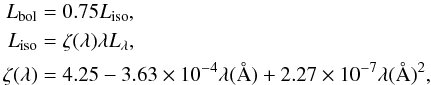 (22)where
λ is the wavelength at rest
and Lλ its corresponding luminosity per
unit wavelength. The expression of an average ζ(λ)
corresponds to a fit to the three values given by Runnoe et al. (2012, Sect. 4.1). The result is shown in Fig. 8. As can be observed, the dispersion is high, most likely owing to the
spread in the values of the real bolometric correction with respect to the given
conversion.
(22)where
λ is the wavelength at rest
and Lλ its corresponding luminosity per
unit wavelength. The expression of an average ζ(λ)
corresponds to a fit to the three values given by Runnoe et al. (2012, Sect. 4.1). The result is shown in Fig. 8. As can be observed, the dispersion is high, most likely owing to the
spread in the values of the real bolometric correction with respect to the given
conversion.
Values of the average kinetic power for different sets of parameters.
In Fig. 8, the correlation is
 (significant at 2.2-σ), where
x ≡ log 10Lbolometric,QSO (erg/s),
and y ≡ log 10PK,total (erg/s).
The correlation is barely significant (97.2% C.L.), but let us accept that the correlation
is there, and again assume that there is no evolution. From a fit to Fig. 8, we get
(significant at 2.2-σ), where
x ≡ log 10Lbolometric,QSO (erg/s),
and y ≡ log 10PK,total (erg/s).
The correlation is barely significant (97.2% C.L.), but let us accept that the correlation
is there, and again assume that there is no evolution. From a fit to Fig. 8, we get  erg/s.
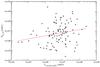 |
Fig. 8 Kinetic power released in jets versus the bolometric luminosity derived from visible luminosities with bolometric corrections. The solid line is the fit indicated in the text. |
The Eddington ratio is  ,
where Lbol is the bolometric luminosity and the Eddington
luminosity
LEddington = 1.3 × 1038MBH(M⊙) erg/s.
The dependence of ϵ on redshift is non-existent or negligible, but there
is a dependence on luminosity for the QSOs for
z < 5 (López-Corredoira & Gutiérrez
2012), given by
,
where Lbol is the bolometric luminosity and the Eddington
luminosity
LEddington = 1.3 × 1038MBH(M⊙) erg/s.
The dependence of ϵ on redshift is non-existent or negligible, but there
is a dependence on luminosity for the QSOs for
z < 5 (López-Corredoira & Gutiérrez
2012), given by
 . With this
relationship and the above result, we get that the average kinetic power is around a
fourth of the Eddington luminosity for a source with
Lbol ~ 1047 erg/s, and the
dependence on the luminosity is small
. With this
relationship and the above result, we get that the average kinetic power is around a
fourth of the Eddington luminosity for a source with
Lbol ~ 1047 erg/s, and the
dependence on the luminosity is small  . We
also note that some source may have super-Eddington kinetic power (see Fig. 7). These are general results applicable to the bright
radio-loud quasars in our present sample.
. We
also note that some source may have super-Eddington kinetic power (see Fig. 7). These are general results applicable to the bright
radio-loud quasars in our present sample.
Other correlations with other luminosities could also be explored, for instance, the correlation with the luminosity of broad emission lines, which is approximately equal to the core radio luminosity (Celotti et al. 1997). Apart from the mass/luminosity and/or redshift, there is also a dependence of the kinetic power on the Bondi accretion rates (Allen et al. 2006), which we did not explore here.
4.2. Possible sources of errors
The calculation of the average kinetic power depends on the value of the different
parameters and, although the preferred values were chosen, we can explore how this average
power changes with other parameters. In Table 1, we
give the values of  for different values of the parameters, except for fsynch: we
show the dependence of the average total kinetic power
on njet, α, Fmin,
Γmax, and aΓ.
for different values of the parameters, except for fsynch: we
show the dependence of the average total kinetic power
on njet, α, Fmin,
Γmax, and aΓ.
The values of fsynch < 0.0103 (corresponding to fewer than 10 electrons per proton) can only increase the kinetic power since it is inversely proportional to fsynch. Nonetheless, an underestimation of the ratio of electrons to protons (Kataoka et al. 2008; Ghisellini & Tavecchio 2010) might also decrease the kinetic power. It is possible that the composition varies with the distance from the main core, but in any case our values reflect an average expected composition on the observed scale.
Another uncertainty might come from the calculation of the blob volume. The beam size is
1.1 × 0.6 mas, and the error in the position of the center of the blob is 0.05 mas (Lister
et al. 2009b). The error in the major
axis 2aj might be a few tenths of mas with
2aj ~ 1 mas; that is, an error of a few
tens per cent. Since, from Eqs. (6), (7), and (19),  ,
this error would not alter the order of magnitude. In addition, since we only see the
front part of the jet, there might a long tail behind that is less luminous due to a lower
Doppler boosting; but this could only increase the volume, leading to a
lower Bmin and higher mass of the jet; hence, a higher
kinetic power.
,
this error would not alter the order of magnitude. In addition, since we only see the
front part of the jet, there might a long tail behind that is less luminous due to a lower
Doppler boosting; but this could only increase the volume, leading to a
lower Bmin and higher mass of the jet; hence, a higher
kinetic power.
We have certainly used here an assumption of the minimum energy, but a change in this hypothesis would not affect the order of magnitude either. All other methods of the kinetic power determination (see Sect. 1) also use either this assumption of minimum energy or the equipartition of energy.
We therefore find that a huge amount of kinetic power is obtained with any set of
parameters. The most significant reduction (of an order of magnitude at most) could be
obtained if we reduced the limiting Γmax to ~ 20 (but always over its minimum
value  ),
or if we allowed as many as ~ 100 electrons per proton in the plasma.
),
or if we allowed as many as ~ 100 electrons per proton in the plasma.
5. Comparison with other works, discussion, and conclusions
Celotti et al. (1997), Ma et al. (2008), and Gu et al. (2009) obtain both a kinetic power of quasars on pc-scales on the same order that we obtained here, and similar correlations with the luminosity. Nonetheless, as said in Sect. 1, their kinetic power estimations correspond to energy fluxes (including both kinetic and internal energies) crossing the section of the observed jet per unit time at the moment in which it is observed, whereas our calculation tells us about the rate of total energy released in the form of kinetic energy by the quasar in the long term.
Rafferty et al. (2006) and Merloni & Heinz
(2007) compiled a list of measured kinetic powers
on kpc-scales based on the nuclear properties of sub-Eddington AGNs, estimating the kinetic
power from the pdV work done to inflate the cavities and
bubbles observed in the hot X-ray-emitting atmospheres of their galaxies and clusters.
Merloni & Heinz (2007) obtained a dependence
with the radio luminosity (uncorrected of Doppler boosting, as in our case) similar to ours
of KR = (8.7 ± 1.4) × 1046 erg/s,
and βR = 0.54 ± 0.09. However, the dependence
on the black hole mass is very different. If we take the data of kinetic power compiled in
Table 1 of Merloni & Heinz (2007), and we
perform the fit versus black hole mass, we get  erg/s.
Here, the exponent might be compatible, but the amplitude is much lower in Merloni &
Heinz than in our sample of Fig. 7, leading to a
factor 103 of difference. This lower amplitude may be caused by the use of
their sample of sub-Eddington AGNs, which is a mixture of BL Lac objects and low Eddington
ratio quasars, since our quasars with higher average Eddington ratios are expected to have
higher kinetic powers for the same black hole mass. However, it may also be caused by our
direct measurement of the kinetic power giving a much higher power than the direct
measurement obtained by analyzing cavities in the X-ray gas.
erg/s.
Here, the exponent might be compatible, but the amplitude is much lower in Merloni &
Heinz than in our sample of Fig. 7, leading to a
factor 103 of difference. This lower amplitude may be caused by the use of
their sample of sub-Eddington AGNs, which is a mixture of BL Lac objects and low Eddington
ratio quasars, since our quasars with higher average Eddington ratios are expected to have
higher kinetic powers for the same black hole mass. However, it may also be caused by our
direct measurement of the kinetic power giving a much higher power than the direct
measurement obtained by analyzing cavities in the X-ray gas.
Using radio observations, and assuming that radio lobes store most of the kinetic power via work done by the expanding radio source, Xu et al. (2009) calculate the kinetic powers of their sample of quasars. The average kinetic power for quasars with black hole masses of 109 M⊙ is ~ 5 × 1044f3/2 erg/s, with f a factor between 1 and 20 (Willott et al. 1999). Even for the highest allowed value of f, their kinetic power is lower than ours (see Fig. 7). We said in Sect. 4.2 that we could reduce an order of magnitude of value of the amplitude, for instance allowing 100 electrons/proton instead of 10. Within an uncertainty of one order of magnitude for our kinetic power, our results fit the value of Xu et al. (2009). If our high values of the kinetic power on parsec-scales were confirmed, it would imply that the extragalactic jets are more powerful than previously estimated from lobe energies and ages, or that there is a significant energy-loss from the parsec to the kiloparsec-scales. The latter is possible if the amount of energy in thermal particles in the lobes is underestimated by the equipartition assumption (e.g., Punsly 2005). Nevertheless, we bear in mind that the different samples refer to different ranges of redshifts and the evolution could also explain the differences. In reality, the possibility that a large fraction of the energy in the lobes is in the form of thermal (invisible) particles has already been suggested (Ito et al. 2008) and evidence of metal-enriched gas has been found along the jets of several radio sources (Kirkpatrick et al. 2009, 2011). If the relation between these results is confirmed, we may be able to infer important implications for the mass-load of extragalactic jets.
We have found that the kinetic power is a significant portion of the Eddington luminosity
![Mathematical equation: \hbox{$\left[\frac{p_{\rm K,total}}{L_{\rm Eddington}} \sim 0.2 \times \left(\frac{L_{\rm bol}}{10^{47}{\rm~erg/s}}\right)^{-0.3}\right]$}](/articles/aa/full_html/2012/08/aa19410-12/aa19410-12-eq208.png) ,
and on the order of the bolometric luminosity. It is proportional on average
to
,
and on the order of the bolometric luminosity. It is proportional on average
to  ; the
correlation with bolometric luminosity is also similar, although less significant. In any
case, these correlations might be affected by Malmquist bias or other selection effects.
Once again, we recall that these results are valid for our sample of radio-loud quasars with
relatively high luminosities and the range of redshifts between 0.15 and 3.4 (half of the
sample with z < 1 and half of the sample with
z > 1); we do not know whether these results can
be extrapolated to other kinds of AGNs and whether some evolution might produce different
results in different redshift ranges.
; the
correlation with bolometric luminosity is also similar, although less significant. In any
case, these correlations might be affected by Malmquist bias or other selection effects.
Once again, we recall that these results are valid for our sample of radio-loud quasars with
relatively high luminosities and the range of redshifts between 0.15 and 3.4 (half of the
sample with z < 1 and half of the sample with
z > 1); we do not know whether these results can
be extrapolated to other kinds of AGNs and whether some evolution might produce different
results in different redshift ranges.
With regard to the probabilistic question mentioned in Sect. 1, we find from this analysis a distribution of superluminal sources observed by the MOJAVE collaboration (Lister et al. 2009b) in which from 354 observed blobs (down to 5 mJy in 101 quasars) 95% are superluminal and 45% are observed with projected velocities more than ten times the speed light. There is a huge excess of jets ejected in a direction close to the line of sight. This can be explained as a selection effect in which both the core and the blobs are affected by huge enhancements of fluxes produced by Doppler boosting, which makes the probability of finding that a jet is ejected within 10 degrees of the line of sight ≳ 40 times higher than one would expect for a random distribution of ejections.
Acknowledgments
We are grateful for the helpful comments of Eduardo Ros, José Ma. Martí, and the anonymous referee. We thank the text corrections by Claire Halliday (A&A language editor). This research has made use of data from the MOJAVE database that is maintained by the MOJAVE team (Lister et al. 2009a). This research has made use of the NASA/IPAC Extragalactic Database (NED), which is operated by the Jet Propulsion Laboratory, California Institute of Technology, under contract with the National Aeronautics and Space Administration. MLC was supported by the grant AYA2007-67625-CO2-01 of the Spanish Science Ministry. MP acknowledges the financial support of the Spanish “Ministerio de Ciencia e Innovación” (MICINN) grants AYA2010-21322-C03-01, AYA2010-21097-C03-01, and CONSOLIDER2007-00050.
References
- Allen, S. W., Dunn, R. J. H., Fabian, A. C., Taylor, G. B., & Reynolds, C. S. 2006, MNRAS, 372, 21 [NASA ADS] [CrossRef] [Google Scholar]
- Bell, M. B. 2012, Int. J. Astron. Astrophys., 2, 52 [CrossRef] [Google Scholar]
- Blandford, R. D., & Königl, A. 1979, ApJ, 232, 34 [NASA ADS] [CrossRef] [Google Scholar]
- Cattaneo, A., Faber, S. M., Binney, J., et al. 2009, Nature, 460, 213 [NASA ADS] [CrossRef] [PubMed] [Google Scholar]
- Celotti, A., Padovani, P., & Ghisellini, G. 1997, MNRAS, 286, 415 [NASA ADS] [CrossRef] [EDP Sciences] [Google Scholar]
- Cohen, M. H., & Unwin, S. C. 1984, in VLBI and Compact Radio Sources, IAU Symp. 110, eds. R. Fanti, K. Kellermann, & G. Setti (Dordrecht: Reidel), 95 [Google Scholar]
- Cohen, M. H., Cannon, W., Purcell, G. H., et al. 1971, ApJ, 170, 207 [NASA ADS] [CrossRef] [Google Scholar]
- De Young, D. S. 2010, ApJ, 710, 743 [NASA ADS] [CrossRef] [Google Scholar]
- Fabian, A. C., Sanders, J. S., Taylor, G. B., et al. 2006, MNRAS, 366, 417 [Google Scholar]
- Ghisellini, G. 2000, in Recent Developments in General Relativity, eds. B. Casciaro, D. Fortunato, M. Francaviglia, & A. Masiello (Berlin: Springer), 5 [Google Scholar]
- Ghisellini, G. 2011, 25th Texas Symposium on Relativistic Astrophysics (New York: AIP, Melville), AIP Conf. Proc., 1381, 180 [Google Scholar]
- Ghisellini, G., & Tavecchio, F. 2010, MNRAS, 409, L79 [NASA ADS] [CrossRef] [Google Scholar]
- Gu, M., Cao, X., & Jiang, D. R. 2009, MNRAS, 396, 984 [NASA ADS] [CrossRef] [Google Scholar]
- Gubbay, J., Legg, A. J., Robertson, D. S., et al. 1969, Nature, 224, 1094 [NASA ADS] [CrossRef] [Google Scholar]
- Ito, H., Kino, M., Kawakatu, N., Isobe, N., & Yamada, S. 2008, ApJ, 685, 828 [NASA ADS] [CrossRef] [Google Scholar]
- Kataoka, J., Madejski, G., Sikora, M., et al. 2008, ApJ, 672, 787 [NASA ADS] [CrossRef] [Google Scholar]
- Katz-Stone, D. M., & Rudnick, L. 1997, ApJ, 488, 146 [NASA ADS] [CrossRef] [Google Scholar]
- Kino, M., & Kawakatu, N. 2005, MNRAS, 364, 659 [NASA ADS] [Google Scholar]
- Kirkpatrick, C. C., Gitti, M., Cavagnolo, K. W., et al. 2009, ApJ, 707, L69 [NASA ADS] [CrossRef] [Google Scholar]
- Kirkpatrick, C. C., McNamara, B. R., & Cavagnolo, K. W. 2011, ApJ, 731, L23 [NASA ADS] [CrossRef] [Google Scholar]
- Knight, C. A., Robertson, D. S., Rogers, A. E. E., et al. 1971, Science, 172, 52 [NASA ADS] [CrossRef] [Google Scholar]
- Königl, A. 2010, IJMPD, 19, 635 [NASA ADS] [CrossRef] [Google Scholar]
- Lister, M. L., & Marscher, A. P. 1997, ApJ, 476, 572 [NASA ADS] [CrossRef] [Google Scholar]
- Lister, M. L., Aller, H. D., Aller, M. F., et al. 2009a, AJ, 137, 3718 [NASA ADS] [CrossRef] [Google Scholar]
- Lister, M. L., Cohen, M. H., Homan, D. C., et al. 2009b, AJ, 138, 1874 [NASA ADS] [CrossRef] [Google Scholar]
- Liu, Y., & Zhang, S. N. 2007, ApJ, 667, 724 [NASA ADS] [CrossRef] [Google Scholar]
- López-Corredoira, M. 2011, Int. J. Astron. Astrophys., 1, 73 [Google Scholar]
- López-Corredoira, M., & Gutiérrez, C. M. 2012, RAA, 12, 249 [NASA ADS] [Google Scholar]
- Ma, M.-L., Cao, X.-W., Jiang, D.-R., & Gu, M.-F. 2008, Chin. J. Astron. Astrophys., 8, 39 [Google Scholar]
- McNamara, B. R., & Nulsen, P. E. J. 2007, ARA&A, 45, 117 [NASA ADS] [CrossRef] [MathSciNet] [Google Scholar]
- McNamara, B. R., Nulsen, P. E. J., Wise, M. W., et al. 2005, Nature, 433, 45 [NASA ADS] [CrossRef] [PubMed] [Google Scholar]
- Merloni, A., & Heinz, S. 2007, MNRAS, 381, 589 [NASA ADS] [CrossRef] [Google Scholar]
- Narlikar, J. V., & Chitre, S. M. 1984, J. Astrophys. Astr., 5, 495 [NASA ADS] [CrossRef] [Google Scholar]
- Perucho, M., & Martí, J. M. 2002, ApJ, 568, 639 [NASA ADS] [CrossRef] [Google Scholar]
- Perucho, M., Agudo, I., Gómez, J. L., et al. 2008, A&A, 489, L29 [NASA ADS] [CrossRef] [EDP Sciences] [Google Scholar]
- Perucho, M., Quilis, V., & Martí, J. M. 2011, ApJ, 743, 42 [NASA ADS] [CrossRef] [Google Scholar]
- Punsly, B. 2005, ApJ, 623, L9 [NASA ADS] [CrossRef] [Google Scholar]
- Pushkarev, A. B., Kovalev, Y. Y., Lister, M. L., & Savolainen, T. 2009, A&A, 507, L33 [NASA ADS] [CrossRef] [EDP Sciences] [Google Scholar]
- Rafferty, D. A., McNamara, B. R., Nulsen, P. E. J., & Wise, M. W. 2006, ApJ, 652, 216 [NASA ADS] [CrossRef] [Google Scholar]
- Rawlings, S., & Saunders, R. 1991, Nature, 349, 138 [NASA ADS] [CrossRef] [Google Scholar]
- Rees, M. 1966, Nature, 211, 468 [NASA ADS] [CrossRef] [Google Scholar]
- Runnoe, J. C., Brotherton, M. S., & Shang, Z. 2012, MNRAS, 422, 478 [NASA ADS] [CrossRef] [Google Scholar]
- Ryle, M., & Longair, M. S. 1967, MNRAS, 136, 123 [NASA ADS] [CrossRef] [Google Scholar]
- Schneider, D. P., Richards, G. T., Hall, P. B., et al. 2010, AJ, 139, 2360 [NASA ADS] [CrossRef] [Google Scholar]
- Shen, Y., Richards, G. T., Strauss, M. A., et al. 2011, ApJS, 194, 45 [NASA ADS] [CrossRef] [Google Scholar]
- Vermeulen, R. C., & Cohen, M. H. 1994, ApJ, 430, 467 [NASA ADS] [CrossRef] [Google Scholar]
- Waldram, E. M., Pooley, G. G., Davies, M. L., Grainge, K. J. B., & Scott, P. F. 2010, MNRAS, 404, 1005 [NASA ADS] [CrossRef] [Google Scholar]
- Whitney, A. R., Shapiro, I. I., Rogers, A. E. E., et al. 1971, Science, 173, 225 [NASA ADS] [CrossRef] [Google Scholar]
- Willott, C. J., Rawlings, S., Blundell, K. M., & Lacy, M. 1999, MNRAS, 309, 1017 [NASA ADS] [CrossRef] [Google Scholar]
- Xu, Y.-D., Cao, X., & Wu, Q. 2009, ApJ, 694, L107 [NASA ADS] [CrossRef] [Google Scholar]
- Young, A. J., Wilson, A. S., & Mundell, C. G. 2002, ApJ, 579, 560 [NASA ADS] [CrossRef] [Google Scholar]
- Zanni, C., Murante, G., Bodo, G., et al. 2005, A&A, 429, 399 [NASA ADS] [CrossRef] [EDP Sciences] [Google Scholar]
Appendix A: Total kinetic energy, including the unobserved ejections due to low energy
The energy EK,obs. is the statistical average of the kinetic energy of the ejected blobs we have observed, but there are other ejections that cannot be observed because their flux density Fj is lower than the detection limit Fmin. We can only see the ejections with high values of Γj because the rest of them have insufficient Doppler boosting to make them observable. The number of observed blobs correspond to the average number of expected blobs with Fj > Fmin, where Fmin is the minimum flux density required to be observable.
Hence, the fraction of kinetic energy within the observed blobs (assuming
P(Γ) ∝ ΓaΓ; Liu & Zhang
2007) is 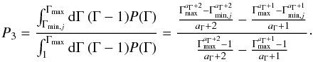 (A.1)This minimum Lorentz
factor Γmin,j at which the blob is observed is related to
the minimum flux Fmin and the intrinsic flux
density F0,j by means of Eq. (4)
(A.1)This minimum Lorentz
factor Γmin,j at which the blob is observed is related to
the minimum flux Fmin and the intrinsic flux
density F0,j by means of Eq. (4)
![Mathematical equation: \appendix \setcounter{section}{1} \begin{equation} F_{\min} = \frac{F_{0,j}}{\left[\Gamma_{{\rm min},j} \left(1-\beta \left(\Gamma _{{\rm min},j}\right)\cos \theta_j\right)\right]^{n_{\rm jet}-\alpha }} \cdot \end{equation}](/articles/aa/full_html/2012/08/aa19410-12/aa19410-12-eq216.png) (A.2)Using again Eqs. (4)
for F0,j, and Eq. (2), and solving the quadratic equation (with
the sign “−”, which has the physical meaning of a minimum Γ), we get
(A.2)Using again Eqs. (4)
for F0,j, and Eq. (2), and solving the quadratic equation (with
the sign “−”, which has the physical meaning of a minimum Γ), we get
![Mathematical equation: \appendix \setcounter{section}{1} \begin{eqnarray} \Gamma_{{\rm min},j} &= \frac{K_{\min} -\sqrt{\cos^2\theta_j\left(K_{\min}^2-\sin^2\theta_j\right)}} {\sin ^2\theta_j}, \nonumber\\[1.5mm] K_{\min} &= \left[\Gamma_j \left(1-\beta_j\cos \theta_j\right)\right] \left(\frac{F_j}{F_{\min}}\right)^{\frac{1}{n_{\rm jet}-\alpha}}, \end{eqnarray}](/articles/aa/full_html/2012/08/aa19410-12/aa19410-12-eq217.png) (A.3)provided
that Γmin,j < Γ, otherwise the values
of Γj, θj are
not valid.
(A.3)provided
that Γmin,j < Γ, otherwise the values
of Γj, θj are
not valid.
The total kinetic energy, both from the jets we see and the jets that we do not see, is
the result of dividing the energy of each observed blob by
P3(Γj,θj).
In the case of the data in this paper, for which the minimum flux density for the
detection of a blob is Fmin = 5 mJy, we have calculated that
 with an r.m.s. of 1.0. We
include this effect in our calculations in this paper because it is important for
some QSOs with low P3.
with an r.m.s. of 1.0. We
include this effect in our calculations in this paper because it is important for
some QSOs with low P3.
Appendix B: Conical jets
If the jets were emitted in a cone with a significant width, we would have to perform a new correction to the calculation of the total energy, since the observed energy only accounts for the ejections with low values of θj and the rest of them have insufficient Doppler boosting to make them observable. The number of observed jets correspond to the average number of expected jets with Fj > Fmin,j, where Fmin is the minimum flux density required to be observable.
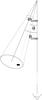 |
Fig. B.1 Representation of the cone within which the jets move, and the blobs (filled black spot) are produced. The azimuthal angles (φ, φcone) are not represented. |
The blobs are within a cone of solid angle ωcone, as
represented in Fig. B.1. We must integrate over all
possible values of the axis of the cone (θcone,
φcone) for a given approaching direction
(θcone < π/2),
and once the cone is fixed, we integrate over all the possible directions of the ejection
within that cone. Hence, the probability of observing an approaching jet is  (B.1)where
Ω1 ≡ conic solid angle around
(θj,φj = 0)
of ωcone stereo radians with
θcone < π/2,
Ω2 ≡ conic solid angle around
(θcone,φcone)
of ωcone stereo radians, such that
θ < θmin,j.
(B.1)where
Ω1 ≡ conic solid angle around
(θj,φj = 0)
of ωcone stereo radians with
θcone < π/2,
Ω2 ≡ conic solid angle around
(θcone,φcone)
of ωcone stereo radians, such that
θ < θmin,j.
The minimum angle θmin,j at which the blob
is observed is related to the minimum flux Fmin and the
intrinsic flux density F0,j by means of
Eq. (4)
![Mathematical equation: \appendix \setcounter{section}{2} \begin{equation} F_{\min} = \frac{F_{0,j}}{\left[\Gamma_j\left(1-\beta_j\cos \theta_{{\rm min},j}\right)\right]^{n_{\rm jet}-\alpha}}\cdot \end{equation}](/articles/aa/full_html/2012/08/aa19410-12/aa19410-12-eq236.png) (B.2)Thus, using again
Eqs. (4) for
F0,j, and Eq. (3), we get
(B.2)Thus, using again
Eqs. (4) for
F0,j, and Eq. (3), we get
 (B.3)Using spherical
trigonometric relations, Eq. (A.1) can be
rewritten as
(B.3)Using spherical
trigonometric relations, Eq. (A.1) can be
rewritten as ![Mathematical equation: \appendix \setcounter{section}{2} \begin{eqnarray} & P_4\left(\Gamma_j, \theta_j\right) = \frac{4}{\omega_{\rm cone}^2}\int_{\max \left[0,\left(\theta_j-\rho _{\rm core}\right)\right]}^{\min\left[\pi /2, \left(\theta_j + \rho_{\rm core}\right)\right]}{\rm d}\theta_{\rm cone} \int_0^{\rho_{\rm cone}}{\rm d}\theta_{\rm c}' \nonumber\\[2mm] &\qquad \times \sin \theta _{\rm cone}\sin \theta_{\rm c}' \nonumber\\[2mm] &\qquad \times \cos^{-1}\left[\max \left(-1,\frac{\cos \rho_{\rm cone}-\cos \theta _{\rm cone}\cos \theta_j}{\sin \theta _{\rm cone}\sin \theta_j}\right)\right] \nonumber\\[2.25mm] &\qquad \times \cos^{-1}\left[\max \left(-1,\min \left(1,\frac{\cos \theta _{{\rm min},j}-\cos \theta _{\rm cone}\cos \theta _{\rm c}'}{\sin \theta _{\rm cone}\sin \theta _{\rm c}'}\right)\right)\right] \cdot \end{eqnarray}](/articles/aa/full_html/2012/08/aa19410-12/aa19410-12-eq238.png) (B.4)We
note that θcone is an angle with respect to line of sight,
whereas
(B.4)We
note that θcone is an angle with respect to line of sight,
whereas  is an angle with
respect to the axis of the cone. The angular radius ρcone
stands for the semiangle of the cone
is an angle with
respect to the axis of the cone. The angular radius ρcone
stands for the semiangle of the cone
 (B.5)The kinetic power, both
from the jets we see and the jets we do not see, results from dividing the energy of each
observed
(B.5)The kinetic power, both
from the jets we see and the jets we do not see, results from dividing the energy of each
observed
blob by P4. Nonetheless, given that from MOJAVE data ρcone = 0.13/Γ ≪ 1 (Pushkarev et al. 2009), we find that P4 ≈ 1 and the correction is negligible. Had ρcone a high value (for instance, in the model by Blandford & Königl 1979, ρcone = 1/Γ), we would have to apply this correction for low values of the Lorentz factor Γ.
All Tables
All Figures
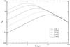 |
Fig. 1 Values of βapp for different values of θ and Γ following Eq. (3). |
| In the text | |
|
Fig. 2 Values of the enhancement of the flux in a blob (Doppler boosting), F/F0, for different values of θ and Γ following Eq. (4), assuming njet − α = 2. |
| In the text | |
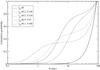 |
Fig. 3 Cumulative probability |
| In the text | |
|
Fig. 4 Probability distribution of the Lorentz factor for a jet with an observed projected linear velocity (in units of c) of βapp = 6.74, as in the case of QSO 0016+731. |
| In the text | |
|
Fig. 5 Histogram of the distribution of kinetic power derived with Eq. (19) for the 101 quasars of the MOJAVE complete sample (Lister et al. 2009a,b). |
| In the text | |
|
Fig. 6 Kinetic power released in jets versus the radio luminosity of the parent quasar. The solid line is the fit indicated in the text. |
| In the text | |
|
Fig. 7 Kinetic power released in jets versus the mass of the black hole of the parent quasar for the cases in common between MOJAVE sample and SDSS-DR7. The solid line indicates the Eddington luminosity. |
| In the text | |
|
Fig. 8 Kinetic power released in jets versus the bolometric luminosity derived from visible luminosities with bolometric corrections. The solid line is the fit indicated in the text. |
| In the text | |
|
Fig. B.1 Representation of the cone within which the jets move, and the blobs (filled black spot) are produced. The azimuthal angles (φ, φcone) are not represented. |
| In the text | |
Current usage metrics show cumulative count of Article Views (full-text article views including HTML views, PDF and ePub downloads, according to the available data) and Abstracts Views on Vision4Press platform.
Data correspond to usage on the plateform after 2015. The current usage metrics is available 48-96 hours after online publication and is updated daily on week days.
Initial download of the metrics may take a while.