| Issue |
A&A
Volume 544, August 2012
|
|
|---|---|---|
| Article Number | A85 | |
| Number of page(s) | 12 | |
| Section | Interstellar and circumstellar matter | |
| DOI | https://doi.org/10.1051/0004-6361/201219320 | |
| Published online | 02 August 2012 | |
Morphology of the very inclined debris disk around HD 32297⋆
1
LESIA, Observatoire de Paris, CNRS, University Pierre et Marie Curie Paris
6 and University Denis Diderot Paris 7,
5 place Jules Janssen,
92195
Meudon,
France
e-mail: This email address is being protected from spambots. You need JavaScript enabled to view it.
2
Institut de Planétologie et d’Astrophysique de Grenoble,
Université Joseph Fourier, CNRS, BP 53, 38041
Grenoble,
France
3
European Southern Observatory, Casilla 19001, Santiago 19, Chile
Received:
30
March
2012
Accepted:
27
June
2012
Abstract
Context. Direct imaging of circumstellar disks at high angular resolution is mandatory to provide morphological information that constrains their properties, in particular the spatial distribution of dust. For a long time, this challenging objective was, in most cases, only within the realm of space telescopes from the visible to the infrared. New techniques combining observing strategy and data processing now allow very high-contrast imaging with 8-m class ground-based telescopes (10-4 to 10-5 at ~1′′) and complement space telescopes while improving angular resolution at near infrared wavelengths.
Aims. We present the results of a program carried out at the VLT with NACO to image known debris disks with higher angular resolution in the near-infrared than ever before in order to study morphological properties and ultimately detect the signpost of planets.
Methods. The observing method makes use of advanced techniques of adaptive optics, coronagraphy, and differential imaging, a combination designed to directly image exoplanets with the upcoming generation of “planet finders” such as GPI (Gemini Planet Imager) and SPHERE (Spectro-Polarimetric High contrast Exoplanet REsearch). Applied to extended objects such as circumstellar disks, the method is still successful but produces significant biases in terms of photometry and morphology. We developed a new model-matching procedure to correct for these biases and hence provide constraints on the morphology of debris disks.
Results. From our program, we present new images of the disk around the star HD 32297 obtained in the H (1.6 μm) and Ks (2.2 μm) bands with an unprecedented angular resolution (~65 mas). The images show an inclined thin disk detected at separations larger than 0.5−0.6″. The modeling stage confirms a very high inclination (i = 88°) and the presence of an inner cavity inside r0 ≈ 110 AU. We also find that the spine (line of maximum intensity along the midplane) of the disk is curved, which we attribute to a large anisotropic scattering-factor (g ≈ 0.5, which is valid for an non-edge-on disk).
Conclusions. Our modeling procedure is relevant to interpreting images of circumstellar disks observed with angular differential imaging. It allows us to both reduce the biases and estimate the disk parameters.
Key words: stars: individual: HD 32297 / stars: early-type / techniques: image processing / techniques: high angular resolution
Based on observations collected at the European Southern Observatory, Chile, ESO (385.C-0476(B)).
© ESO, 2012
1. Introduction
Many stars have photometric infrared (IR) excesses that can be attributed to the presence of circumstellar dust. Among the circumstellar disk evolution, the debris disk phase is the period where most of the primordial gas has been dissipated or accreted onto already formed giant planets. The dust content responsible for the IR excesses is thought to be the result of regular mutual collisions between asteroid-like objects and/or the evaporation of cometary bodies (Wyatt 2008; Krivov 2010). This activity, presumably triggered by unseen planets, is continuously replenishing the system with observable dust grains that, in turn, trace out the presence of a planetary system. The direct imaging detection of planets in circumstellar disks around main-sequence A-type stars such as β Pictoris (Lagrange et al. 2010) and HR 8799 (Marois et al. 2008b) or the undefined point-source around Fomalhaut (Kalas et al. 2008; Janson et al. 2012) has clearly revealed the long suspected close relation between planet formation and debris-disk structures (Ozernoy et al. 2000; Wyatt 2003; Reche et al. 2008). Moreover, the most prominent structures in these specific disks (warp, annulus, gap, offset) can be accounted for by the mass and orbital properties of these associated planets. Similar features are seen in other debris disks where planets have not yet been imaged. Many disks are thought to have internal cavities attributed to dust sweeping by planets. From a face-on to an edge-on geometry, these structures are more or less easily identified. Therefore, a morphological analysis is mandatory to study disk evolution, planetary formation, and the likely presence of planets.
Log of observations summarizing the parameters.
HD 32297 is a young A5 star that was identified with an IR excess (LIR/L∗ = 0.0027) by IRAS and later resolved as a inclined circumstellar debris disk by Schneider et al. (2005) in the near IR with NICMOS on HST. Observations in the visible (R band) were obtained by Kalas (2005) and revealed a circumstellar nebulosity at distances larger than 560 AU, that was interpreted as a broad scattered-light region extending to 1680 AU. The brightness asymmetries and a distorted morphology are indicative of an interaction with the interstellar medium. Hubble Space Telescope (HST) data obtained at 1.1 μm probe the inner region within ~400 AU and as close as 34 AU from the star (corresponding to, respectively, 3.3′′ and 0.3′′). Schneider et al. (2005) derived a position angle (PA) of 47.6 ± 1.0° and an inclination of about 10° from edge-on. A surface brightness (SB) asymmetry is also observed in the southwest (SW) side of the disk, which is about twice brighter than the northeast (NE) side at a projected angular separation of about 0.3−0.4′′. Observations at mid-IR wavelengths (11.7 μm and 18.3 μm) performed by Moerchen et al. (2007) indicate that there has been dust depletion closer than ~70 AU suggesting there is an inner cavity similar to the one found in either HR 4796 (Schneider et al. 1999) or HD 61005 (Buenzli et al. 2010), but with a less steep decrease in density. However, this radius is poorly constrained in the mid-IR as the equivalent resolution corresponds to from 35 AU to 50 AU at the HD 32297 distance. Additional colors were obtained by Debes et al. (2009) at 1.60 μm and 2.05 μm again with NICMOS, which confirms the previous measurement of the disk orientation (PA = 46.3 ± 1.3° at NE and 49.0 ± 2.0° at SW). The SB profiles confirm the asymmetries and reveal a slope break at 90 AU (NE) and 110 AU (SW). If similar to some other disks such as β Pictoris (Augereau et al. 2001) and AU Mic (Augereau & Beust 2006), this break indicates the boundary of a planetesimal disk, and is marginally compatible with the value (70 AU) derived by Moerchen et al. (2007), even though the measurements may not be directly comparable to that of Schneider et al. (2005). In addition it has been shown that the disk midplane is curved at separations larger than 1.5′′ (170 AU), possibly as the result of the interaction with the interstellar medium. This probably impacts the PA measurement. More recently, Mawet et al. (2009) achieved very high-contrast imaging of the disk with a small (1.6 m) well-corrected sub-aperture at the Palomar in Ks and confirmed the color and brightness asymmetry, although the lower angular resolution did not allow them to perform a detailed morphological study.
At a distance of 113 ± 12 pc (Perryman et al. 1997), the disk of HD 32297 is of particular interest for probing the regions where planets would have formed on the 10-AU scale provided that high angular resolution and high contrast are achieved simultaneously. In this paper, we present new diffraction-limited images of the HD 32297 debris disk in the near-IR (1.6 μm and 2.2 μm) using an 8-m class telescopewith adaptive optics, hence a significant improvement with respect to former observations (of a factor of about three on the angular resolution at the same wavelengths). We note that similar observations obtained at the Keck telescope in the same near-IR bands are presented by Esposito et al. (2012). Section 2 presents the results of the observation. In Sect. 3, we analyze the reliability of a particular structure observed in the image. Section 4 provides the surface brightness profiles of the disk before biases are taken into account. The core of this paper is presented in Sect. 5, where we attempt to identify the disk parameters. In Sect. 6, the surface brightness corrected for the observational bias is derived. Finally, we present constraints on the presence of point sources within the disk.
2. Observation and data reduction
2.1. Observations
The star HD 32297 (A5, V = 8.13, H = 7.62, K = 7.59, near-IR values are from the Two Micron All Sky Survey) was observed with NACO (Nasmyth Adaptive Optics System and Near-Infrared Imager and Spectrograph), the near-IR AO-assisted camera at the Very Large Telescope (VLT, Rousset et al. 2003; Lenzen et al. 2003), on 25 September 2010 UT using a dedicated strategy to allow for high contrast imaging. We combined two modes offered in NACO: the four-quadrant phase mask coronagraphs (FQPMs, Rouan et al. 2000) to attenuate the on-axis star, and the pupil tracking mode to allow for angular differential imaging (ADI, Marois et al. 2006). We used the broad-band filters H and Ks for which the FQPMs are optimized (Boccaletti et al. 2004) and the S27 camera providing a sampling of ~0.027′′ per pixel. Coronagraphic images were obtained with a field stop of 8 × 8′′ and 13 × 13′′ in, respectively, H and Ks and an undersized pupil stop of 90% of the full pupil diameter. Phase masks already provided interesting results on both extended objects (Riaud et al. 2006; Boccaletti et al. 2009; Mawet et al. 2009) and point sources as companion to stars (Boccaletti et al. 2008; Serabyn et al. 2010; Mawet et al. 2011).
The log of observations is shown in Table 1. The integration time of individual FQPM exposures (DIT) was chosen to fill about 80% of the dynamical range of the detector (including the attenuation by the coronagraph), and the duration of a template (DIT × NDIT) does not exceed 30 s, so as to enable us to correct for a systematic drift correlated with the parallactic angle variations in pupil tracking mode. Therefore, the star is re-aligned with the coronagraphic mask every 30 s when needed (the drift increases closer to the meridian). At the end of the sequence, a few sky frames were acquired around the target star. As for calibration purposes, we obtained out-of-mask images of the star itself with a neutral density filter (but without the undersized stop) to determine the point-spread function (PSF), which is intended to normalize coronagraphic images, hence calculate either SB or contrast curves. In addition, since the phase masks are engraved on a glass substrate, their transmission map is measured with a flat illumination provided by the internal lamp of NACO. Seeing conditions were good to medium: 0.72 ± 0.06′′ in Ks and 0.97 ± 0.12′′ in H. The AO correction provides a FWHM (full width at half maximum) of ~65 mas in both filters, while theoretical values for an 8-m class telescope at the longest wavelengths of the H and Ks bands are 46 mas and 59 mas, respectively. Therefore, images are nearly diffraction-limited in Ks as opposed to H.
In pupil tracking, while the field rotates, the smearing of off-axis objects is faster at the edge of the field. However, for a few seconds of integration per frame, the smearing is totally negligible within our field of view.
2.2. Data reduction and results
The data were reduced with our own pipeline. We first applied bad pixel removal and flat-field correction to every frame. Although quite faint here, we averaged sky frames and subtracted a background map (including the dark) as it reduces the offset. Given the large amount of coronagraphic images and to save computing time, we binned the data cubes to reduce their size. We adopted a binning step of five frames (averaging) while keeping the ADI-induced smearing still negligible. A median sky frame was subtracted from every binned frames. We then rejected the frames of the poorest quality with a flux criteria (for instance open AO loop), and obtained data cubes of 129 (75% of data) and 158 (69% of data) frames for, respectively, the Ks and H band data, representing a total integration time of 1290 and 1706 s, respectively. The frame recentering is a non-linear problem, because the star moves behind the coronagraph so that the intensity and shape of the residual pattern vary significantly. It is therefore impossible to apply a standard centroiding algorithm and the issues are different from those in saturated imaging (Lagrange et al. 2012a). In particular, the FQPM creates four peaks of unequal intensities from which it is difficult to extract an astrometric signal since phase aberrations are also quite large and perturb the coronagraphic image. We tested several procedures, focusing on the fitting of the halo. The best result was obtained when the individual frames were thresholded to 10% of the image maximum and a Moffat profile was fitted so as to give more weight to some pixels in the stellar halo than those closer to the star. In this way, we achieved a sub-pixel accuracy for centering but were unable to determine a reliable mean to estimate a value. Finally, we used the background image of the FQPM alone to apply a correction derived from its own flat-field image to every re-centered frame.
Following the nomenclature described in Lagrange et al. (2012a), we processed the data with several ADI algorithms, which differ in the way in which they build a reference frame:
-
Classical ADI (cADI, Marois et al. 2006), which subtracts the median of the datacube to each frame.
-
Radial ADI (rADI, Marois et al. 2006; Lafrenière et al. 2007) for which a set of reference frames to be subtracted is determined separately on each annulus. The algorithm is controlled by the separation criterion, which defines in a deterministic way the time lapsed between one frame and its reference frames, together with the amount of field rotation.
-
Locally Optimized Combination of Images (LOCI, Lafrenière et al. 2007) is more sophisticated since it defines optimization zones (with a particular geometry) where the reference frame to be subtracted (in a zone smaller than the optimization one) is estimated as a linear combination of all frames for which the field object has moved by the desired quantity (separation criterion Nδ). Optimization zones are larger than the subtraction zones for limiting the subtraction of a potential point source. Several parameters control the LOCI algorithm, but the most relevant here are the separation criterion and the size of the optimization zone.
As circumstellar disks are extended objects, these techniques are not optimized since they favor the detection of unresolved sources and apply to different independent zones in the image breaking of the continuous shape of a disk. Nevertheless, they can be very efficient in emphasizing regions with strong gradients of similar spatial scales as point sources (rings for instance). In the past few years, several impressive results were obtained using ADI and revealed the very detailed structures within some debris disks (Buenzli et al. 2010; Thalmann et al. 2011; Lagrange et al. 2012a,b). Self-subtraction is an important issue and is caused by the contribution of the disk itself to the building of the reference image to be subtracted from the data cube. Because of the field rotation, the inner regions of a circumstellar disks are more affected by self-subtraction in the ADI processing since they cover smaller angular sectors. Moreover, the self-subtraction of the disk increases as the algorithm ability to suppress speckles improves (LOCI being more aggressive than cADI for instance). This is particularly important in our data since the rotation amplitude is less than 25°. A detailed analysis of the self-subtraction arising when imaging disks with ADI will be presented in Milli et al. (submitted).
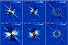 |
Fig. 1 Final images of the disk around HD 32297 in the Ks (top) and H (bottom) bands for the cADI, rADI, and LOCI (left to right) algorithms (see Sect. 2.2 for acronyms). The field of view of each sub-image is 3 × 3″. The color bar indicates the contrast with respect to the star per pixel (which is not applicable to the display-saturated central residuals). |
Angular differential imaging algorithms can produce a wealth of various images across which both the stellar residuals and the signal of the object will be modulated. The adjustment of the parameters relies on the balance between self-subtraction and the separation from the star at which the disk is detected. This qualitative analysis leads us to set the separation criterion for both rADI and LOCI to 1.0 × FWHM and 1.5 × FWHM for, respectively, the Ks and H bands, where FWHM = 65 mas in both filters. The radial width is 2 × FWHM for both the LOCI subtraction zones and rADI rings. As for LOCI, we adopt the geometry described in Lafrenière et al. (2007) where the zones are distributed centro-symmetrically. Subtraction zones have a radial to azimuth size factor of unity. The optimization zones start at the same radius as the subtraction zones but extend to larger radii with a total area of NA = 300 × PSF cores. To build the reference image in each zone, all the available frames were used and the coefficients were calculated with a singular value decomposition.
A first look at the resulting images shown in Fig. 1 indicates that (1) no information is retrieved at separations closer than 0.5−0.6′′ since stellar residuals still dominate the image (for instance, the cADI images display a strong waffle pattern as an imprint of the AO system), (2) the H band data are of lower quality than in Ks (as expected from AO performance, see Sect. 2.1, and seeing variations, see Table 1) but LOCI efficiently reduces the stellar residuals at similar radii in both bands, (3) the disk has about the same thickness through all algorithms especially in the Ks band which favors a thin and highly inclined disk, and (4) the H and Ks morphologies are very similar. The structure of stellar residuals changes according to the algorithm, and differs notably from the well-known speckled pattern, especially owing to the azimuthal averaging caused by the de-rotation of the frames. A closer inspection shows that, although the disk is quite linear, it features a small deviation from the midplane more evident in LOCI images to the NE side (especially in Ks but also in H). Figure 2 shows the position of the midplane (red line) with respect to the spine of the disk. The deviation can be clearly seen in the middle of this image and spans several resolution elements (from ~0.6′′ to ~1.0′′). The main objective of the paper is to find a disk morphological model that can account for this deviation. In addition, we present signal-to-noise-ratio (S/N) maps in Fig. 3. The noise level was estimated azimuthally on LOCI images (both H and Ks), which are smoothed with a Gaussian (of FWHM = 65 ms) so as to derive the S/N per resolution element. We achieved detection levels from about 10σ to 20σ along the disk midplane. We caution that the noise estimation can be biased, especially in the speckle-dominated regime close to the star as explained in Marois et al. (2008a). In the case of Fig. 3, this occurs at distances closer than 0.5 ~ 0.6″, although a few speckles still appear further out as significant patterns in the H band S/N map. Finally, we note that the deviation from the midplane is also visible in the S/N maps.
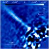 |
Fig. 2 Upper left 1 × 1′′ quadrant of the Ks LOCI image, which emphasizes the deviation away from to the midplane (red line, PA = 47.4°). The star is at the lower-right corner. The color bar indicates the contrast with respect to the star per pixel (which is not applicable to the display-saturated central residuals). |
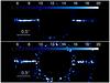 |
Fig. 3 Signal-to-noise map obtained from LOCI images in Ks (top) and H (bottom) for S/N > 5σ per resolution element. The field of view is 4′′ × 1.5′′ and the disk is derotated (PA = 47.4°) to ensure that the disk is aligned along the horizontal. The outer (>1.5″) and inner (<0.6″) regions are excluded. The color bar indicates the S/N per resolution elements. |
3. Morphological analysis
3.1. Position angle determination
We first measured the PA of the disk to check its consistency with the values reported previously by Schneider et al. (2005) and Debes et al. (2009), and with the goal of improving the accuracy owing to the higher angular resolution and the use of the ADI processing. To achieve this, we followed the approach presented in Boccaletti et al. (2009) and more recently in Lagrange et al. (2012a) for the case of β Pictoris, as it is nearly edge-on as the one around HD 32297. The image is de-rotated by an angle corresponding to a rough estimation of the PA (guess) so that the disk is about horizontal with respect to pixels. A vertical fitting by a Gaussian profile along the columns yields for each separation the position of the spine (trace of the maximum SB along the midplane) at a sub-pixel precision. From the position of the spine as a function of radius (smoothed over 4 pixels ≈ 2 FWHM), we then estimated the slope of the spine in four regions carefully chosen to reduce the influence of stellar residuals and background noise. The measurements were made in the regions of 25−40, 25−50, 30−40, and 30−50 pixels (corresponding to a range of 0.675−1.35′′) on each side of the disk together (assuming that the disk crosses the star).
The process is repeated for several angles within a range of 2° sampled at 1/100° around the estimated PA. Finally, the spine slope as a function of this angle shows a steep minimum that unambiguously defines (to a precision of 0.2°) the PA of the disk. We repeated the same analysis for all the images in Fig. 1 and averaged the values. The error bar is calculated from the dispersion in the values to which we quadratically added the celestial north uncertainty (0.2°, according to Lagrange et al. 2012a). We found PA = 47.4 ± 0.3° in the Ks band and PA = 47.0 ± 0.3° in the H band, which agree within the error bars but we adopt the former value since Ks data are of much higher quality. These numbers compare adequately to previous reports but achieve higher precision. However, we did not observe a PA variation of about 3° between the two sides of the disk unlike Debes et al. (2009), but we performed our measurement at closer separations than in HST so the studies are not directly comparable.
3.2. Reliability of the spine deviation from midplane
Following the observation reported in the previous section, our main objective was to
test whether the deviation of the midplane seen in Figs. 1 and 2 could be a bias produced by the ADI
algorithms. Therefore, to overcome this issue and to transform observed measurements into
physical ones requires calibration using models. On the basis of our images, unlike HST
ones, we are insensitive to the regions where the disk is posited to interact with the
interstellar medium (ISM) because of the lower sensitivity at large separations. Hence, we
assumed a simple geometrical model of a ring-like dust disk. We used the GRaTer code
(Augereau et al. 1999; Lebreton et al. 2012) to calculate synthetic scattered-light images of
optically thin disks, assuming axial symmetry about their rotation axis, and inject these
models into the real data. In this study, we assumed a dust number density of (in
cylindrical coordinates): ![Mathematical equation: \begin{eqnarray} n(r,z) = n_0 \sqrt{2}\left[\left(\frac{r}{r_0}\right)^{-2\alpha_{\rm in}} + \left(\frac{r}{r_0}\right)^{-2\alpha_{\rm out}}\right]^{-\frac{1}{2}} \exp{\left(\left(\frac{-|z|}{H_0\left(\frac{r}{r_0}\right)^{\beta}}\right)^{\gamma}\right)}, \end{eqnarray}](/articles/aa/full_html/2012/08/aa19320-12/aa19320-12-eq51.png) (1)where
n0 and H0 are the midplane
number-density and the disk scale-height at the reference distance to the star
r = r0, respectively. The slopes
αin and αout were chosen such
that the density is rising with increasing distance up to r0
and decreasing beyond (αin ≥ 0 and
αout ≤ 0). This was intended to mimic a dust belt with a
peak density position close to r0, a geometry appropriate for
cold debris disks in isolation (that have no interaction with the ISM). A ray-traced image
was then calculated assuming a disk inclination i from pole-on viewing,
and anisotropic scattering modeled by an Henyey &
Greenstein (1941) phase function with asymmetry parameter g
between −1 (pure backward scattering) and 1 (forward scattering). To limit the number of
free parameters, we assumed a Gaussian vertical profile (γ = 2) with a
scale-height proportional to the distance to the star (β = 1). At this
stage, we generated a limited number of models with some assumptions about the remaining
free parameters taken from the literature (Schneider
et al. 2005; Moerchen et al. 2007; Debes et al. 2009), namely g = 0
(isotropic scattering), r0 = 70 AU,
αout = −4, H0 = 2 AU,
i = [80,85,88] °, and
αin = [0,2] . The vertical height
H0 is consistent with the natural thickening of debris disks
defined by Thébault (2009), although chosen close
to the lower boundary of the proposed range in that paper. Hence, in our case, the aspect
ratio was assumed to be constant at
H/r ≃ 0.029. We note that the
simplified version of GRaTer used in this study is unable to handle perfectly edge-on
viewing i = 90°.
(1)where
n0 and H0 are the midplane
number-density and the disk scale-height at the reference distance to the star
r = r0, respectively. The slopes
αin and αout were chosen such
that the density is rising with increasing distance up to r0
and decreasing beyond (αin ≥ 0 and
αout ≤ 0). This was intended to mimic a dust belt with a
peak density position close to r0, a geometry appropriate for
cold debris disks in isolation (that have no interaction with the ISM). A ray-traced image
was then calculated assuming a disk inclination i from pole-on viewing,
and anisotropic scattering modeled by an Henyey &
Greenstein (1941) phase function with asymmetry parameter g
between −1 (pure backward scattering) and 1 (forward scattering). To limit the number of
free parameters, we assumed a Gaussian vertical profile (γ = 2) with a
scale-height proportional to the distance to the star (β = 1). At this
stage, we generated a limited number of models with some assumptions about the remaining
free parameters taken from the literature (Schneider
et al. 2005; Moerchen et al. 2007; Debes et al. 2009), namely g = 0
(isotropic scattering), r0 = 70 AU,
αout = −4, H0 = 2 AU,
i = [80,85,88] °, and
αin = [0,2] . The vertical height
H0 is consistent with the natural thickening of debris disks
defined by Thébault (2009), although chosen close
to the lower boundary of the proposed range in that paper. Hence, in our case, the aspect
ratio was assumed to be constant at
H/r ≃ 0.029. We note that the
simplified version of GRaTer used in this study is unable to handle perfectly edge-on
viewing i = 90°.
Images of the models were first convolved with the observed PSF(obtained with the ND filter but no stop). While the field rotates, the orientation of the disk changes with respect to some PSF features (spiders and static phase aberrations). Hence, a model should rigorously be first rotated at a given orientation and then convolved with the PSF, and the convolution repeated for each parallactic angle in the data cube. We checked, however, that our conclusions were unaffected when the convolution was applied once and the convolved model rotated. The AO-correction quality is likely not good enough in this particular case to make a difference. We adopted this faster solution to save computing time. Model disks were inserted at 90° from the observed disk so there was no possible overlap in-between. A similar strategy was adopted by Thalmann et al. (2011). We used the same approach as described above for measuring the PA. The fitting of the observed and model-disk vertical profiles versus radius yields the disk spine position, vertical thickness, and intensity. Vertical thickness appears to be a good criterion to disentangle between several disk inclinations (i parameter). Figure 4 plots the vertical thickness (FWHM of a Gaussian) measured on the observed disk (black line) and the model disks (colored lines) for the three inclinations and the three algorithms. Qualitatively, we found that the closest match with the models is achieved for an inclination of i = 88°. This will be confirmed in the next section with a more precise model fitting but already seems different from the values of Schneider et al. (2005) where 77° ≤ i ≤ 82°. In addition, we note that the shape of the FWHM profiles as a function of radius was quite well-reproduced with the model, providing support to a constant disk aspect ratio. This suggests that the disk is open beyond about 1′′. Finally, for this particular inclination of 88°, we measured a minimal observed vertical thickness for the observed and model disks of about 0.07′′ at a distance of about 0.85′′ (96 AU) in the cADI images. This is consistent with the value of H0 used in the model given the effect of the inclination and the convolution with the PSF.
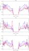 |
Fig. 4 Width of the observed disk (black line) in Ks for cADI (top), rADI (middle), and LOCI (bottom) images, compared to the width of the model for i = 80° (blue line), i = 85° (magenta line), and i = 88° (red line). The NE side is at the left. |
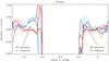 |
Fig. 5 Spine of the disk in Ks for the observed disk (blueish lines), and the i = 88° model (reddish lines) as measured in cADI, rADI, and LOCI. The elevation from the midplane is measured for PA = 47.4°. Arrows indicate where the deviation to the midplane is observed. The NE side is at the left. |
Figure 5 shows for the most likely inclination (i = 88°), the disk spine position for cADI, rADI, and LOCI images in Ks and for both the observed and model disks. The deviation from the midplane can be most clearly seen on the NE side for Ks images between 0.6′′ and 1′′ and reaches a maximum of 0.025″ (~1 pixel). The deviation has on average an amplitude of about 0.015′′ and spans across 15 pixels (which is about 6 resolution elements). The noise level per resolution element is equivalent to about 0.005′′. Therefore, the deviation from the midplane is significant at the ~7.5σ level. A low-significance symmetrical deviation is barely also seen in the SW side with the same amplitude. In H-band images, the deviation is more difficult to detect. It is still visible on the NE side only in the rADI and LOCI images. There is also a possible deviation at larger radii (>1.2″) on both sides and towards the NW, which may comply with the change in PA noted by Debes et al. (2009) although our data are far less deep than HST in these regions to permit us to confirm this. We checked that other models mostly lead to the same conclusion. In addition, we found that the deviation in the NE side at 0.6−1′′ is unaffected by a variation in the PA within the error bars (0.3°).
Finally, as the LOCI performs locally the injection of model disks at 90° from the observed disk, the procedure might be inappropriate for calibrating the bias of the algorithm. In the LOCI images of Fig. 1, we calculated instead the coefficients of the linear combinations for each zone, applied them to a model disk of the same PA as the observed disk (but in an empty data cube), and still observed a nearly flat midplane of the model disk in the 0.6−1′′ region. To summarize, an inclined model disk with a symmetrical vertical intensity distribution with respect to the midplane (g = 0, i < 90°) produces the same symmetry in the ADI-processed images. Therefore, the shape of the midplane observed in Figs. 1, 2, and 5 is definitely not due to a bias of the ADI process but is real. Interestingly and as additional evidence, images acquired by Esposito et al. (2012) from Keck reveal (at least qualitatively) the same deviation from the midplane at the same separations.
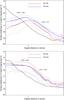 |
Fig. 6 Surface brightness expressed in mag/arcsec2 as measured in the H band (top) and Ks band (bottom). Red and blue lines stand for the NE and SW sides, respectively. Dotted lines show the disk intensity dispersion at 1σ within the slit window of 0.25′′. The black line indicates the noise level measured out of the slit window. Dashed lines correspond to the fitted power-law profile next to which the slopes are indicated. |
4. Photometric analysis
The photometric analysis of a disk observed in ADI can be problematic, especially when as in our case the field rotation is small. The ADI effect can be understood in the resulting image as a transmission map projected on the sky in which the pattern depends on the disk brightness distribution. For instance, it is interesting to note in Lagrange et al. (2012a) that LOCI produces on the disk of β Pic a very strong attenuation, only because it is very well-resolved in the vertical dimension. The actual brightness distribution of the disk is therefore needed to properly account for this attenuation and derive reliable measures. This is the motivation behind the modeling described in the next section. The SB profiles presented in this section cannot be assumed to represent the true photometry but does provide a useful starting point.
As a first step, we performed the SB measurement on cADI images as cADI produces less self-subtraction than other algorithms, hence smaller photometric/astrometric biases. The cADI image of the disk is smoothed over four pixels, and isolated in a narrow slit of 0.25′′ in width aligned along the disk PA. From that, we extracted the mean intensity profile of the disk azimuthally averaged in angular sectors as well as the intensity dispersion, and plot the results in Fig. 6. In doing so and given the edge-on geometry, the intensity mean and dispersion are hence calculated in pixels located at the same physical distances from the star (same flux received) but different elevations from the midplane. In addition, we did the same measurement out of the slit to derive the noise level. There is a clear break in the SB profiles near 1′′ (about 110 AU) between a nearly flat (or even positive) profile inwards and a negative slope outwards. The slopes given in Table 2 are measured at specific positions that we consider to be the most relevant: 0.6−0.9′′ for the inner slopes and 1.2−1.8′′ for the outer slopes. The inner slopes clearly have lower significances because (1) they are measured across only 0.3′′, which is equivalent to 11 pixels (4.5 resolution elements); and (2) this region has higher speckle noise (as indicated by the noise level in Fig. 6). The error bar in the SB slopes can indeed be large considering the intensity dispersion plotted in Fig. 6. To be conservative, we adopt an uncertainty of ±0.5 for the index of the slopes. The inner slope is steeper in H than in Ks, but this result is uncertain given the noise level for such separations, as seen in Fig. 1. The outer slopes are very similar for the two sides of the disk (within the error bars), but noticeably steeper in Ks than in H, as already noted by Debes et al. (2009). The disk also appears dimmer in H than in Ks, which might again be consistent with HST data. As in the case of β Pictoris, we may expect that the disk of HD 32297 contains a planetesimal belt at radii smaller than ~110 AU, which produces dust particles blown away from the system by the radiation pressure of the star (Augereau et al. 2001). Outer slopes close to −4 are compatible with such an assumption.
Slopes (as fitted to power laws) of the different components in the SB of cADI images.
5. Disk modeling
5.1. Parameter space
We now explore whether the morphology of the disk can be accounted for by a model of scattered light images. Using GRaTer (Augereau et al. 1999), we generated a grid of 576 models of which the parameters span relevant values (based on previous guesses) for the disk of HD 32297 as given below:
-
inclination (i): 82, 85, 88, 89.5°;
-
peak density position (r0): 80, 90, 100, 110, 120 AU;
-
power law index of the outer density (αout): −4, −5, −6;
-
power law index of the inner density (αin): 2, 5, 10;
-
anisotropic scattering factor (g): 0, 0.25, 0.50, 0.75.
5.2. Global minimization
As for the global minimization, we isolated the relevant part of the disk with a slit
centered on the disk PA, respectively, PA+90° for the model, 0.5′′
in width for Ks, respectively, 0.3′′ in H and
restrained the radius to the range 0.65−2′′ for H and
Ks. These numbers were carefully chosen to retain only the pixels
containing flux from the observed disk and hence optimize the minimization. For each
model, we then used a standard χ2 metric as follows:
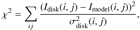 (2)where
Idisk and Imodel are the images
of the observed disk and that of the model for the retained pixels (i,j),
and
(2)where
Idisk and Imodel are the images
of the observed disk and that of the model for the retained pixels (i,j),
and  is derived from the
azimuthal dispersion of Idisk to account for the errors. As we
run the minimization on both sides NE/SW of the disk simultaneously, it implicitly assumes
that the disk is symmetrical about the minor axis. The χ2
minimum usually helps us to determine the model that most closely matches the data, but to
prevent any degeneracies among model parameters we selected instead the 10 lowest minima
corresponding to 10 sets of model parameters per ADI algorithm. Combining the three
algorithms amounts to 30 sets of parameters. It would be inappropriate to derive either
average values or error bars since our grid of models is discrete and cannot be
interpolated. We instead searched independently for each parameter among these sets which
of the value has the highest occurrence as a measure of the significance (value with the
highest occurrence/30). This quantity is a number between 0 and 1 and does not convey any
assumption about the error bar. The results are given in Table 3 for both H and Ks. In the particular
case of r0, we found that both 110 and 120 AU were equally
probable in the Ks image. The significance (indicated in parentheses in
Table 3) has to be larger than the inverse of the
number of allowed values for each parameter. Some parameters are very well-constrained
such as i and g (at least in Ks),
supporting a quite large inclination of 88°. The value for
r0 is in very good agreement with the slope break in the SB
measured by Debes et al. (2009) as in our
measurement (on average of 110 AU). Density profiles are more difficult to constrain,
especially αin, where both H and
Ks are inconsistent but we may expect for these parameters either
chromatic dependences or NE/SW differences. Finally, the global minimization clearly
points to a noticeable anisotropic scattering of g = 0.5. Minimization in
H and Ks leads to the same values for
i, r0, and g, although the
significance is always lower in H as a result of the lower data quality.
is derived from the
azimuthal dispersion of Idisk to account for the errors. As we
run the minimization on both sides NE/SW of the disk simultaneously, it implicitly assumes
that the disk is symmetrical about the minor axis. The χ2
minimum usually helps us to determine the model that most closely matches the data, but to
prevent any degeneracies among model parameters we selected instead the 10 lowest minima
corresponding to 10 sets of model parameters per ADI algorithm. Combining the three
algorithms amounts to 30 sets of parameters. It would be inappropriate to derive either
average values or error bars since our grid of models is discrete and cannot be
interpolated. We instead searched independently for each parameter among these sets which
of the value has the highest occurrence as a measure of the significance (value with the
highest occurrence/30). This quantity is a number between 0 and 1 and does not convey any
assumption about the error bar. The results are given in Table 3 for both H and Ks. In the particular
case of r0, we found that both 110 and 120 AU were equally
probable in the Ks image. The significance (indicated in parentheses in
Table 3) has to be larger than the inverse of the
number of allowed values for each parameter. Some parameters are very well-constrained
such as i and g (at least in Ks),
supporting a quite large inclination of 88°. The value for
r0 is in very good agreement with the slope break in the SB
measured by Debes et al. (2009) as in our
measurement (on average of 110 AU). Density profiles are more difficult to constrain,
especially αin, where both H and
Ks are inconsistent but we may expect for these parameters either
chromatic dependences or NE/SW differences. Finally, the global minimization clearly
points to a noticeable anisotropic scattering of g = 0.5. Minimization in
H and Ks leads to the same values for
i, r0, and g, although the
significance is always lower in H as a result of the lower data quality.
Best-fit model parameters with the global minimization.
 |
Fig. 7 Images of the best-fit disk model (PA = 137.4°) in Ks compared to the observed disk (PA = 47.4°) with cADI, rADI, and LOCI algorithms (left to right). The field of view of each sub-image is 3 × 3′′. Color bars indicate the contrast with respect to the star per pixel (which is not applicable to the display-saturated central residuals). |
5.3. Minimization of surface brightness slopes and spine
The global minimization approach is useful for getting a global picture of the disk because it takes into account all the available information in all the relevant pixels and tries to simultaneously adjust all the model parameters, assuming that the disk is symmetric with respect to the minor axis. However, since the intensity scaling of the model with respect to the observed disk can be problematic (as explained in the previous sub-section), we tested alternative procedures. To refine the analysis, as a second step, we carry out the minimization with other criteria that are less dependent on pixel-to-pixel variations. Here, we set the inclination to i = 88° as a clear outcome of the global minimization analysis.
Starting with the SB we proceed in a similar way to Sect. 4 to extract this quantity from both the observed and model disks. We do not minimize the full SB profile but just the slopes in the four areas of interest inward and outward of 1′′ and independently on the NE and SW sides. We used the same regions defined in Sect. 4 to minimize αout and αin, so that 1.2−1.8′′ and 0.6−0.9′′, respectively. The minimization again provides 30 sets of parameters for each area and we searched for the highest occurrence. The results are shown in Table 4. The analysis of αout shows a steeper index in the NE, but differs for Ks and H and remains in agreement with the SB profiles of the observed disk plotted in Fig. 6. The inner density indices are inconsistent with the global minimization, although with greater significance and converge instead to an intermediate value of αin = 5. The parameter r0 is more affected by dispersion. We concluded that these values are unrepresentative since the range of r0 falls unequally between the two regions where the minimization is performed. However, in this particular case, it is informative to use a mean instead of the highest occurrence since the allowed values for r0 are more finely sampled than the other parameters. This mean is much closer to 110 AU, in concordance with the global minimization. Furthermore, the minimization of SB slopes is inappropriate for constraining the anisotropic scattering factor since the dispersion between the solutions is too large (0.00 < g < 0.75).
Best-fit model parameters with the SB minimization.
Best-fit model parameters with the spine minimization.
One last measurement was carried out to more tightly constrain the anisotropic scattering factor. We applied the procedure described in Sect. 3 to evaluate the spine of the disk as we consider it can provide a more accurate estimation of the anisotropic scattering factor, even though it is potentially correlated to other parameters such as the densities. For the same reasons as above, we expect these geometrical measurements to be less dependent on the intensity normalization of the model disks. Results are reported in Table 5, where we considered the NE and SW sides separately. Here, we did not expect to derive significant results for αout and αin, which are related to the disk intensity while we measure only the coordinates of the spine. This is confirmed in Table 5 where no particular value emerges. The radius r0 shows a difference between the NE (110−120 AU) and SW (80−90 AU) sides (although with a low significance for Ks) that actually agrees with the images where the NE side appears to be slightly more elongated than the SW side. Debes et al. (2009) also noted such a NE/SW asymmetry but in the opposite direction. However, they directly used the indication of this from the SB without performing any modeling. Orbital motion of a hypothetical structure at such a separation is totally inconsistent between the two epochs. As the disk is seen almost edge-on, this asymmetry could be related to a stellocentric offset of the central cavity, as in many other debris disks (Boccaletti et al. 2003; Kalas et al. 2005; Thalmann et al. 2011; Lagrange et al. 2012b), and then interpreted as a signpost of a planet sculpting the disk. The relation between this potential offset and the anisotropic scattering remains to be explored. As for the factor g, the Ks band favors one single value of 0.25, while it is larger in H. We note that the largest value of the anisotropic scattering factor (g = 0.75) is actually unrealistic according to our images since it would make the disk brighter than the stellar residuals in the zone r < 0.65″. As we exclude this region dominated by the starlight in the minimization process, the relevant pixels where large values of g contribute are missed and hence some large values may come out. It is surprising that the spine minimization yields a different value for g than the global minimization (0.25 instead of 0.50) while remaining symmetrical. Nevertheless, the global minimization converges to g = 0.50 with a much higher significance, at least in Ks.
5.4. Discussion
The determination of the model parameters is imperfect in the case of our data given the S/N ratio of the images, while we also expect some degeneracies in-between some parameters. The disk of HD 32297 being close to edge-on, the inclination is definitely the easiest parameter to measure. We found an optimal value of i = 88°, which is larger than the original measure with HST data and makes the disk more inclined than previously thought. This difference of inclination can possibly explain, and hence actually supports, the scenario of interaction with the ISM (Debes et al. 2009) which has noticeable effect on the HST data because of its higher sensitivity to faint source. We then found that r0 and g are derived with quite good significance, at least for the global and spine minimizations. For some parameters, it is reasonable to assume a higher weight from the images in Ks, which are of much higher quality than in the H band. Considering an axisymmetrical disk, we retained the values of the global minimization r0 = 110 AU and g = 0.50 as the optimal numbers to describe the disk morphology. It is more difficult to constrain the indices of the density profiles. First of all, within a radius of r0 the number of pixels used to fit a slope is small. The 0.6−0.9′′ region used corresponds to only about 11 pixels in radius. Second, the noise introduced by the residual, corresponding to unattenuated starlight produces bumpiness in the SB that can easily affect the measurement of the slope exponent by 1, while it is the level of precision we would like to determine as imposed by the model parameter sampling. Combining the global and SB minimizations, we choose αout = −5 in Ks. In H, the values of αout are discrepant. The SB minimization, which is in principle more accurate for measuring the SB slopes, points to a lower value. To be consistent with the slopes shown in Fig. 6, we adopt αout = −5 in H. This value is consistent with the predictions of Lecavelier des Etangs et al. (1996) for a circular ring of planetesimals producing dust with collisions and expelled by the radiation pressure. It is also similar to the slopes measured in the debris disk around β Pic (Golimowski et al. 2006). Finally, the values of αin are in practice clearly more difficult to measure but appear systematically larger in H than in Ks. To reproduce such a behavior, we select αin = 5 in H and αin = 2 in Ks.
Table 6 gives the final choice of parameters combining the results presented above in Tables 3–5. As an illustration, a model disk with the parameters determined for the Ks band data is shown in Fig. 7 at 90° from the observed disk. In both filters, the parameters that describe the morphology of the disk as projected on the sky (i, r0 and g) are strictly identical. This is definitely a good indication that the minimization process is performing well. As an additional demonstration, Fig. 8 shows for the maximum inclination allowed by HST measurements (Schneider et al. 2005) that the model would be discrepant with our disk image. If the inclination were i = 82° with no anisotropy, we should see either the inner cavity or a thicker disk depending on αin. With an anisotropic scattering factor identical to our estimate (g = 0.5), the deviation from the midplane would be larger that we measured. The parameters that do indeed depend on the intensities (αout, αin) are in contrast subject to questioning. The difference observed between the two filters can be due to either uncertainties or chromatic dependences. The accuracy of the data does not allow us to firmly decide and these power-law indices generate SB slopes that agree within the error bars with those measured in Fig. 6. However, we note that the depletion of the central cavity is not as steep as other cases such as either HD 61005 (Buenzli et al. 2010) or HR 4796 (Schneider et al. 1999; Lagrange et al. 2012b), as already mentioned by Moerchen et al. (2007) from mid-IR images.
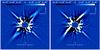 |
Fig. 8 Images of the disk model (PA = 137.4°) in Ks for i = 82° and g = 0, 0.5 (respectively left and right) compared to the observed disk (PA = 47.4°) with rADI. The field of view of each sub-image is 3 × 3′′. Color bars indicate the contrast with respect to the star (which is not applicable to the display-saturated central residuals). |
Best-fit model parameters retained.
6. Surface brightness of the best-fit models
The SB profiles presented in Fig. 6 are impacted by the ADI process, which produces a radial-dependent self-subtraction of the disk. In particular, the parts of the disk that are closer to the star undergo a larger subtraction.
However, since the best-fit model had been identified we could attempt to recover the most likely SB profile corrected for the self-subtraction by measuring it directly from the model after this had been normalized adequately. To perform this, we first compared the cADI image of the observed disk to the cADI image of the best-fit model to determine precisely their intensity ratio. We used this ratio to inject a fake disk into an empty data cube to mimic the field rotation. Instead of processing the data with one of the ADI algorithms, we simply derotated the frames and summed them up. We then applied the same measurement as in Sect. 4. The resulting SB profiles corresponding to the aforementioned parameters are shown in Fig. 9. The SB profiles derived from the models differ significantly from those measured in cADI images. Angular differential imaging has an obvious effect on the slopes of the SB, as also noted in Lagrange et al. (2012b). The net result of the ADI, in our case, is to change the intensity variations along the midplane, sometimes reinforcing the intensity gradient. Starting from a negative inner slope in the models (Fig. 9), it becomes nearly flat (in Ks) or even positive (in H) in the ADI images (Fig. 6). Similarly, the outer slope exponents are increased by ~1. We were unable to reproduce the steepness of the inner profile in H but the negative areas in the images (Fig. 1) suggest that the reference frame subtraction in H has a stronger effect than in Ks1. Finally, the profiles for the models are brighter as expected since the ADI self-subtraction is accounted for. The cADI image in Ks is about 0.3 mag/arcsec2 fainter than the model at 1′′ (corresponding to r0). In H, the attenuation can be as large as ~1 mag/arcsec2 at the same radius.
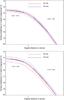 |
Fig. 9 Surface brightness expressed in mag/arcsec2 as measured for the model with parameters i = 88°, r0 = 110 AU, αout = −5, αin = 5, g = 0.50 (top), corresponding to the H band and for the parameters i = 88°, r0 = 110 AU, αout = −5, αin = 2, g = 0.50, corresponding to the Ks band. Red and blue lines stand for the NE and SW sides, respectively. Dotted lines show the disk intensity dispersion at 1σ within the slit window of 0.25′′. Dashed lines correspond to the fitted power-law profile next to which the slopes are indicated. |
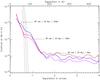 |
Fig. 10 Detection limit to point sources at 5σ for cADI (magenta), rADI (red), and LOCI (blue). The expected intensity of some planetary objects from the BT-SETTL model are shown for an age of 30 Myr (dashed lines). The dotted lines correspond to the mass/separation range of planets able to sculpt the disk assuming that the inner edge of the ring is located at 90, 100, and 110 AU. |
7. Limit of detection to point sources
Our data have the highest contrast ever reported for HD 32297 in the Ks
band near ~1′′, hence are suitable for deriving the detection limit of point
sources in the planet/brown-dwarf mass regime. In this particular case, it is relevant to
measure the contrast along the midplane as the orbits of hypothetical planets will likely be
aligned with the disk plane. For each image in Fig. 1,
the disk is isolated in a 0.3′′ slit window centered on the midplane. The
standard deviation is calculated for the pixels that are vertical to the midplane at each
radii (we check that the result does not strongly depends on the slit width). The
photometric biases introduced by the self-subtraction of the three ADI algorithms were
calibrated with nine fake planets (copy of the PSF) injected into the data cube and located
at specific locations (from 0.25′′ to 5′′ and 90° from the
midplane to avoid confusion with the disk). An attenuation profile was interpolated for
these flux losses, assuming that it varies monotonically with radius (which is not necessary
true for LOCI) and used to correct for photometric biases and provide calibrated contrast
curves. The 5σ contrast curves are presented in Fig. 10. As it is measured in the disk midplane instead of the background
noise, the detection limit is similar for the three algorithms. We also plot the level of
contrast for three planet masses 6, 10, and 20 MJupiter assuming
an age of 30 Myr (Kalas 2005) and considering the
BT-SETTL models from Allard et al. (2011). However, we
note that the age of HD 32297 is not very well-determined. We can definitely reject the
presence of brown dwarfs at separations larger ~50 AU and closer than ~600 AU (FOV
limitation). Owing to the distance of the star (113 pc), it is impossible to put any
constraints on planetary mass objects at closer separations. At 110 AU, the distance of the
inner ring, the detection limit reaches ~10 MJupiter. Assuming
that the inner cavity is sculpted by a planet and following the approach presented in Lagrange et al. (2012b), we can estimate the position of
this hypothetical planet. According to Wisdom (1980)
and Duncan et al. (1989, Eq. (23)), the distance of
the planet to the rim of the ring (δa) is related to the planet/star mass
ratio (Mp/Ms)
with the relation  (3)where
a is the semi-major axis. Hence, a + δa
is the distance to the inner rim, which is smaller than r0. The
same formulation was used by Chiang et al. (2009) in
the case of Fomalhaut b. We calculated Mp for several
assumptions about a + δa (90, 100, 110 AU) and taking
Ms = 2.09M⊙. We interpolated
these masses on the BT-SETTL model, hence converted them into absolute magnitudes and
contrasts. Smaller values of a + δa would lead to
unrealistic masses in the stellar domain. The dotted lines in Fig. 10 show the combination of planet masses and separations that are able to
produce an inner ring at 110 AU. The comparison between dynamical constraints (dotted lines)
and detection limits (solid lines) indicates that there is a possible range of separations
and masses for the planet of a > 65 ~ 85 AU
and Mp < 12 MJupiter.
We stress that this estimation is only valid for a planet at the quadrature (projected
separation = physical separation). However, given the steepness of the dynamical
constraints, if a planet produces the ring it must be close to the rim, otherwise it would
be sufficiently massive to have been detected.
(3)where
a is the semi-major axis. Hence, a + δa
is the distance to the inner rim, which is smaller than r0. The
same formulation was used by Chiang et al. (2009) in
the case of Fomalhaut b. We calculated Mp for several
assumptions about a + δa (90, 100, 110 AU) and taking
Ms = 2.09M⊙. We interpolated
these masses on the BT-SETTL model, hence converted them into absolute magnitudes and
contrasts. Smaller values of a + δa would lead to
unrealistic masses in the stellar domain. The dotted lines in Fig. 10 show the combination of planet masses and separations that are able to
produce an inner ring at 110 AU. The comparison between dynamical constraints (dotted lines)
and detection limits (solid lines) indicates that there is a possible range of separations
and masses for the planet of a > 65 ~ 85 AU
and Mp < 12 MJupiter.
We stress that this estimation is only valid for a planet at the quadrature (projected
separation = physical separation). However, given the steepness of the dynamical
constraints, if a planet produces the ring it must be close to the rim, otherwise it would
be sufficiently massive to have been detected.
8. Summary and conclusions
We have presented high contrast images of the debris disk around HD 32297 obtained with NACO at the VLT in the near-IR H and Ks bands. To improve the attenuation of the starlight and the speckle rejection, we used both phase mask coronagraphy and ADI algorithms. The nearly edge-on disk is detected in the two filters at radial distances from 0.65′′ to 2′′ (from 74 AU to 226 AU at the distance of 113 pc) by applying various ADI algorithms. We have illustrated that ADI is a very efficient method for achieving detection but induces somephotometric biases that have to be corrected for in the data analysis for a proper interpretation. We observed a deviation from the midplane near 0.8′′ on the NE side that is clearly not an ADI bias. We focused our effort on the morphological modeling of the disk using a numerical code GRaTer, which produces synthetic scattered-light images of debris disks. Following previous observations, we considered a disk containing a planetesimal belt with a dust distribution both inward and outward of the belt. We generated a five-parameter grid of models and applied several sorts of minimizations to constrain the disk morphology.
As a first result, we found in Ks and H bands a higher inclination than previously published at 1.1 μm (88° instead of 80°). In our images, the vertical extent of the disk together with the disk parameters found from modeling are definitely inconsistent with such a disk inclination. However, we suspect that the isophotal ellipse-fitting used in previously published data (Schneider et al. 2005) can be biased by the strong interaction with the interstellar medium as revealed by Debes et al. (2009), especially when considering the lower angular resolution and conversely the higher sensitivity to faint structures of NICMOS/HST as opposed to NACO. In addition, we did not find any significant NE/SW brightness asymmetry as in Schneider et al. (2005) and Mawet et al. (2009), although we have also observed at near-IR wavelengths too.
Furthermore, the minimization of the disk parameters has allowed us to constrain the radius of the planetesimal belt at 110 AU. A NE/SW asymmetry is suspected, possibly due to an offset of the planetesimal belt from the star. We have shown that the deviation from the midplane is likely the result of anisotropic scattering. One edge of the disk is therefore brighter. Whether this is linked to either the dust properties or the geometry (the hypothetical offset of the belt) and hence to a gravitational perturber is yet unclear. It is remarkable that among the known debris disks, three of them surround A-type stars, namely, β Pic, Fomalhaut, and HD 32297, while they share the same position of the planetesimal belt near 100 AU as a possible indication of a common architecture.
Intensity-related parameters such as the brightness slopes of the inner and outer parts are more difficult to constrain and the values we determined should be interpreted with caution as the uncertainty can be large. However, it gives an order of magnitude indicating that the outer parts have a power-law index close to that expected for dust grains expelled from the system by radiation pressure. As for the inner parts, there is a significant difference between the Ks and H band filters, but overall, the steepness is shallower than for some other ring-like debris disks, as already noted by Moerchen et al. (2007).
Armed with a detailed morphological characterization, it is now possible to start a dynamical study to understand the properties of the debris disk around HD 32297 in terms of either planetary formation or gravitational perturbation as was performed in other cases (Wyatt 2005; Chiang et al. 2009). Finally, the observations of debris disks from ground-based telescopes in the near-IR are achieving comparable or even higher angular resolution than HST, owing to adaptive optics. A similar statement can be made about contrast thanks to a combination of high-contrast imaging techniques (coronagraphy, ADI). The next generation of extreme adaptive-optics instruments, the so-called planet finders (Beuzit et al. 2008; Macintosh et al. 2008; Hodapp et al. 2008), will not only revolutionize the search and characterization of young long-period planets but also the field of debris disk science pending the arrival of the James Webb Space Telescope (Gardner et al. 2006).
In the H band, the decline close to the axis of the SB as observed in Fig. 6 is caused by the negative pattern that appears in Fig. 1 (bottom left) at a different PA than the disk but still affects the disk. It is due to a poor estimation of the reference image essentially because of the diffraction pattern decorrelation over time. We suspect that this butterfly pattern (positive and negative) is due to the secondary spiders. The angle is very close to the 109° that separates two VLT spiders. This residual pattern is seen in several other NACO images.
Acknowledgments
We would like to thank G. Montagnier at ESO for conducting these observations and A. Lecavelier des Etangs for helpful discussions. We also thanks the referee for a very detailed and useful report.
References
- Allard, F., Homeier, D., & Freytag, B. 2011, in ASP Conf. Ser. 448, eds. C. Johns-Krull, M. K. Browning, & A. A. West, 91 [Google Scholar]
- Augereau, J.-C., & Beust, H. 2006, A&A, 455, 987 [NASA ADS] [CrossRef] [EDP Sciences] [Google Scholar]
- Augereau, J. C., Lagrange, A. M., Mouillet, D., Papaloizou, J. C. B., & Grorod, P. A. 1999, A&A, 348, 557 [NASA ADS] [Google Scholar]
- Augereau, J. C., Nelson, R. P., Lagrange, A. M., Papaloizou, J. C. B., & Mouillet, D. 2001, A&A, 370, 447 [NASA ADS] [CrossRef] [EDP Sciences] [Google Scholar]
- Beuzit, J.-L., Feldt, M., Dohlen, K., et al. 2008, in SPIE Conf. Ser., 7014, [Google Scholar]
- Boccaletti, A., Augereau, J.-C., Marchis, F., & Hahn, J. 2003, ApJ, 585, 494 [NASA ADS] [CrossRef] [Google Scholar]
- Boccaletti, A., Riaud, P., Baudoz, P., et al. 2004, PASP, 116, 1061 [NASA ADS] [CrossRef] [Google Scholar]
- Boccaletti, A., Chauvin, G., Baudoz, P., & Beuzit, J.-L. 2008, A&A, 482, 939 [NASA ADS] [CrossRef] [EDP Sciences] [Google Scholar]
- Boccaletti, A., Augereau, J.-C., Baudoz, P., Pantin, E., & Lagrange, A.-M. 2009, A&A, 495, 523 [NASA ADS] [CrossRef] [EDP Sciences] [Google Scholar]
- Buenzli, E., Thalmann, C., Vigan, A., et al. 2010, A&A, 524, L1 [NASA ADS] [CrossRef] [EDP Sciences] [Google Scholar]
- Chiang, E., Kite, E., Kalas, P., Graham, J. R., & Clampin, M. 2009, ApJ, 693, 734 [Google Scholar]
- Debes, J. H., Weinberger, A. J., & Kuchner, M. J. 2009, ApJ, 702, 318 [NASA ADS] [CrossRef] [Google Scholar]
- Duncan, M., Quinn, T., & Tremaine, S. 1989, Icarus, 82, 402 [NASA ADS] [CrossRef] [Google Scholar]
- Esposito, T., Fitzgerald, M. P., Kalas, P., & Graham, J. R. 2012, in AAS Meeting Abstracts, 219, 344.15 [Google Scholar]
- Gardner, J. P., Mather, J. C., Clampin, M., et al. 2006, Space Sci. Rev., 123, 485 [NASA ADS] [CrossRef] [Google Scholar]
- Golimowski, D. A., Ardila, D. R., Krist, J. E., et al. 2006, AJ, 131, 3109 [NASA ADS] [CrossRef] [Google Scholar]
- Henyey, L. G., & Greenstein, J. L. 1941, ApJ, 93, 70 [NASA ADS] [CrossRef] [Google Scholar]
- Hodapp, K. W., Suzuki, R., Tamura, M., et al. 2008, in SPIE Conf. Ser., 7014 [Google Scholar]
- Janson, M., Carson, J. C., Lafrenière, D., et al. 2012, ApJ, 747, 116 [NASA ADS] [CrossRef] [Google Scholar]
- Kalas, P. 2005, ApJ, 635, L169 [NASA ADS] [CrossRef] [Google Scholar]
- Kalas, P., Graham, J. R., & Clampin, M. 2005, Nature, 435, 1067 [NASA ADS] [CrossRef] [PubMed] [Google Scholar]
- Kalas, P., Graham, J. R., Chiang, E., et al. 2008, Science, 322, 1345 [NASA ADS] [CrossRef] [PubMed] [Google Scholar]
- Krivov, A. V. 2010, Res. Astron. Astrophys., 10, 383 [NASA ADS] [CrossRef] [Google Scholar]
- Lafrenière, D., Marois, C., Doyon, R., Nadeau, D., & Artigau, É. 2007, ApJ, 660, 770 [NASA ADS] [CrossRef] [Google Scholar]
- Lagrange, A.-M., Bonnefoy, M., Chauvin, G., et al. 2010, Science, 329, 57 [NASA ADS] [CrossRef] [PubMed] [Google Scholar]
- Lagrange, A.-M., Boccaletti, A., Milli, J., et al. 2012a, A&A, 542, A40 [NASA ADS] [CrossRef] [EDP Sciences] [Google Scholar]
- Lagrange, A.-M., Milli, J., Boccaletti, A., et al. 2012b, A&A, in press, DOI: 10.1051/0004-6361/201219187 [Google Scholar]
- Lebreton, J., Augereau, J.-C., Thi, W.-F., et al. 2012, A&A, 539, A17 [NASA ADS] [CrossRef] [EDP Sciences] [Google Scholar]
- Lecavelier des Etangs, A., Vidal-Majar, A., & Ferlet, R. 1996, A&A, 307, 542 [NASA ADS] [Google Scholar]
- Lenzen, R., Hartung, M., Brandner, W., et al. 2003, in SPIE Conf. Ser., 4841, eds. M. Iye, & A. F. M. Moorwood, 944 [Google Scholar]
- Macintosh, B. A., Graham, J. R., Palmer, D. W., et al. 2008, in SPIE Conf. Ser., 7015 [Google Scholar]
- Marois, C., Lafrenière, D., Doyon, R., Macintosh, B., & Nadeau, D. 2006, ApJ, 641, 556 [Google Scholar]
- Marois, C., Lafrenière, D., Macintosh, B., & Doyon, R. 2008a, ApJ, 673, 647 [NASA ADS] [CrossRef] [Google Scholar]
- Marois, C., Macintosh, B., Barman, T., et al. 2008b, Science, 322, 1348 [NASA ADS] [CrossRef] [PubMed] [Google Scholar]
- Mawet, D., Serabyn, E., Stapelfeldt, K., & Crepp, J. 2009, ApJ, 702, L47 [NASA ADS] [CrossRef] [Google Scholar]
- Mawet, D., Mennesson, B., Serabyn, E., Stapelfeldt, K., & Absil, O. 2011, ApJ, 738, L12 [NASA ADS] [CrossRef] [Google Scholar]
- Moerchen, M. M., Telesco, C. M., De Buizer, J. M., Packham, C., & Radomski, J. T. 2007, ApJ, 666, L109 [NASA ADS] [CrossRef] [Google Scholar]
- Ozernoy, L. M., Gorkavyi, N. N., Mather, J. C., & Taidakova, T. A. 2000, ApJ, 537, L147 [NASA ADS] [CrossRef] [Google Scholar]
- Perryman, M. A. C., Lindegren, L., Kovalevsky, J., et al. 1997, A&A, 323, L49 [NASA ADS] [Google Scholar]
- Reche, R., Beust, H., Augereau, J.-C., & Absil, O. 2008, A&A, 480, 551 [NASA ADS] [CrossRef] [EDP Sciences] [Google Scholar]
- Riaud, P., Mawet, D., Absil, O., et al. 2006, A&A, 458, 317 [NASA ADS] [CrossRef] [EDP Sciences] [Google Scholar]
- Rouan, D., Riaud, P., Boccaletti, A., Clénet, Y., & Labeyrie, A. 2000, PASP, 112, 1479 [NASA ADS] [CrossRef] [Google Scholar]
- Rousset, G., Lacombe, F., Puget, P., et al. 2003, in SPIE Conf. Ser. 4839, eds. P. L. Wizinowich, & D. Bonaccini, 140 [Google Scholar]
- Schneider, G., Smith, B. A., Becklin, E. E., et al. 1999, ApJ, 513, L127 [NASA ADS] [CrossRef] [Google Scholar]
- Schneider, G., Silverstone, M. D., & Hines, D. C. 2005, ApJ, 629, L117 [NASA ADS] [CrossRef] [Google Scholar]
- Serabyn, E., Mawet, D., & Burruss, R. 2010, Nature, 464, 1018 [NASA ADS] [CrossRef] [Google Scholar]
- Thalmann, C., Janson, M., Buenzli, E., et al. 2011, ApJ, 743, L6 [NASA ADS] [CrossRef] [Google Scholar]
- Thébault, P. 2009, A&A, 505, 1269 [NASA ADS] [CrossRef] [EDP Sciences] [Google Scholar]
- Wisdom, J. 1980, AJ, 85, 1122 [NASA ADS] [CrossRef] [Google Scholar]
- Wyatt, M. C. 2003, ApJ, 598, 1321 [NASA ADS] [CrossRef] [MathSciNet] [Google Scholar]
- Wyatt, M. C. 2005, A&A, 440, 937 [NASA ADS] [CrossRef] [EDP Sciences] [Google Scholar]
- Wyatt, M. C. 2008, ARA&A, 46, 339 [NASA ADS] [CrossRef] [Google Scholar]
All Tables
Slopes (as fitted to power laws) of the different components in the SB of cADI images.
All Figures
|
Fig. 1 Final images of the disk around HD 32297 in the Ks (top) and H (bottom) bands for the cADI, rADI, and LOCI (left to right) algorithms (see Sect. 2.2 for acronyms). The field of view of each sub-image is 3 × 3″. The color bar indicates the contrast with respect to the star per pixel (which is not applicable to the display-saturated central residuals). |
| In the text | |
|
Fig. 2 Upper left 1 × 1′′ quadrant of the Ks LOCI image, which emphasizes the deviation away from to the midplane (red line, PA = 47.4°). The star is at the lower-right corner. The color bar indicates the contrast with respect to the star per pixel (which is not applicable to the display-saturated central residuals). |
| In the text | |
|
Fig. 3 Signal-to-noise map obtained from LOCI images in Ks (top) and H (bottom) for S/N > 5σ per resolution element. The field of view is 4′′ × 1.5′′ and the disk is derotated (PA = 47.4°) to ensure that the disk is aligned along the horizontal. The outer (>1.5″) and inner (<0.6″) regions are excluded. The color bar indicates the S/N per resolution elements. |
| In the text | |
|
Fig. 4 Width of the observed disk (black line) in Ks for cADI (top), rADI (middle), and LOCI (bottom) images, compared to the width of the model for i = 80° (blue line), i = 85° (magenta line), and i = 88° (red line). The NE side is at the left. |
| In the text | |
|
Fig. 5 Spine of the disk in Ks for the observed disk (blueish lines), and the i = 88° model (reddish lines) as measured in cADI, rADI, and LOCI. The elevation from the midplane is measured for PA = 47.4°. Arrows indicate where the deviation to the midplane is observed. The NE side is at the left. |
| In the text | |
|
Fig. 6 Surface brightness expressed in mag/arcsec2 as measured in the H band (top) and Ks band (bottom). Red and blue lines stand for the NE and SW sides, respectively. Dotted lines show the disk intensity dispersion at 1σ within the slit window of 0.25′′. The black line indicates the noise level measured out of the slit window. Dashed lines correspond to the fitted power-law profile next to which the slopes are indicated. |
| In the text | |
|
Fig. 7 Images of the best-fit disk model (PA = 137.4°) in Ks compared to the observed disk (PA = 47.4°) with cADI, rADI, and LOCI algorithms (left to right). The field of view of each sub-image is 3 × 3′′. Color bars indicate the contrast with respect to the star per pixel (which is not applicable to the display-saturated central residuals). |
| In the text | |
|
Fig. 8 Images of the disk model (PA = 137.4°) in Ks for i = 82° and g = 0, 0.5 (respectively left and right) compared to the observed disk (PA = 47.4°) with rADI. The field of view of each sub-image is 3 × 3′′. Color bars indicate the contrast with respect to the star (which is not applicable to the display-saturated central residuals). |
| In the text | |
|
Fig. 9 Surface brightness expressed in mag/arcsec2 as measured for the model with parameters i = 88°, r0 = 110 AU, αout = −5, αin = 5, g = 0.50 (top), corresponding to the H band and for the parameters i = 88°, r0 = 110 AU, αout = −5, αin = 2, g = 0.50, corresponding to the Ks band. Red and blue lines stand for the NE and SW sides, respectively. Dotted lines show the disk intensity dispersion at 1σ within the slit window of 0.25′′. Dashed lines correspond to the fitted power-law profile next to which the slopes are indicated. |
| In the text | |
|
Fig. 10 Detection limit to point sources at 5σ for cADI (magenta), rADI (red), and LOCI (blue). The expected intensity of some planetary objects from the BT-SETTL model are shown for an age of 30 Myr (dashed lines). The dotted lines correspond to the mass/separation range of planets able to sculpt the disk assuming that the inner edge of the ring is located at 90, 100, and 110 AU. |
| In the text | |
Current usage metrics show cumulative count of Article Views (full-text article views including HTML views, PDF and ePub downloads, according to the available data) and Abstracts Views on Vision4Press platform.
Data correspond to usage on the plateform after 2015. The current usage metrics is available 48-96 hours after online publication and is updated daily on week days.
Initial download of the metrics may take a while.