| Issue |
A&A
Volume 544, August 2012
|
|
|---|---|---|
| Article Number | A16 | |
| Number of page(s) | 13 | |
| Section | Astrophysical processes | |
| DOI | https://doi.org/10.1051/0004-6361/201218967 | |
| Published online | 19 July 2012 | |
Secondary cosmic-ray nuclei from supernova remnants and constraints on the propagation parameters
1
INFN – Sezione di Perugia, 06122
Perugia,
Italy
e-mail: This email address is being protected from spambots. You need JavaScript enabled to view it.
2
Physics Department, Torino University and INFN,
10125
Torino,
Italy
e-mail: This email address is being protected from spambots. You need JavaScript enabled to view it.
Received:
6
February
2012
Accepted:
23
March
2012
Abstract
Context. The secondary-to-primary boron-to-carbon (B/C) ratio is widely used to study the cosmic-ray (CR) propagation processes in the Galaxy. It is usually assumed that secondary nuclei such as Li-Be-B are generated entirely by collisions of heavier CR nuclei with the interstellar medium (ISM).
Aims. We study the CR propagation under a scenario where secondary nuclei can also be produced or accelerated by Galactic sources. We consider the processes of hadronic interactions inside supernova remnants (SNRs) and the re-acceleration of background CRs in strong shocks. We investigate their impact in the propagation parameter determination within present and future data.
Methods. Analytical calculations are performed in the frameworks of the diffusive shock acceleration theory and the diffusive halo model of CR transport. Statistical analyses are performed to determine the propagation parameters and their uncertainty bounds using existing data on the B/C ratio, as well as the simulated data expected from the AMS-02 experiment.
Results. The spectra of Li-Be-B nuclei emitted from SNRs are harder than those due to CR collisions with the ISM. The secondary-to-primary ratios flatten significantly at ~TeV/n energies, both from spallation and re-acceleration in the sources. The two mechanisms are complementary to each other and depend on the properties of the local ISM around the expanding remnants. The secondary production in SNRs is significant for dense background media, n1 ≳ 1 cm-3, while the amount of re-accelerated CRs is relevant to SNRs expanding into rarefied media, n1 ≲ 0.1 cm-3. Owing to these effects, the diffusion parameter δ may be underestimated by a factor of ~5–15%. Our estimations indicate that an experiment of the AMS-02 caliber can constrain the key propagation parameters, while breaking the source-transport degeneracy for a wide class of B/C-consistent models.
Conclusions. Given the precision of the data expected from ongoing experiments, the SNR production/acceleration of secondary nuclei should be considered, if any, to prevent a possible mis-determination of the CR transport parameters.
Key words: acceleration of particles / nuclear reactions, nucleosynthesis, abundances / cosmic rays / ISM: supernova remnants
© ESO, 2012
1. Introduction
The problems of the origin and propagation of the charged cosmic rays (CRs) in the Galaxy are among the major topics of resarch in modern astrophysics. It is generally accepted that primary CR nuclei such as H, He, C, N, and O, are accelerated in supernova remnants (SNRs) via diffusive shock acceleration (DSA) mechanisms, that produce power-law momentum spectra (Drury 1983). At relativistic energies, S ∝ p−ν ~ E−ν. After being accelerated, CRs are released in the circumstellar environment, where they diffuse through the turbulent magnetic fields and interact with interstellar matter (ISM) (Strong et al. 2007). Owing to diffusion, CRs stream out from the Galaxy on a characteristic timescale τesc ∝ E−δ. The spectrum of primary CR nuclei predicted at Earth is therefore Np ~ Sτesc. The collisions of these nuclei with interstellar gas are believed to be the mechanism producing the secondary CR nuclei, such as Li, Be, and B, which are under-abundant in the thermal ISM. Thus, the equilibrium spectra of secondary CRs are E−δ times softer than those of their progenitors. At energies above some tenths of GeV per nucleon, where CR nuclei reach the pure diffusive regime, this picture predicts power-law distributions such as Np ~ E−ν − δ for primary nuclei and Ns/Np ~ E−δ for secondary-to-primary ratios at Earth. These trends may be straightforwardly derived from the analytical solutions of Maurin et al. (2001). Present observations indicate that δ ~ 0.3–0.7 and ν ~ 2.0–2.4. The bulk of the data is collected at E ≲ 10 GeV nucleon-1, where the CR spectra are shaped by additional effects such as diffusive reacceleration, galactic wind convection, energy losses, and solar modulation. Since there is no firm theoretical prediction of the key parameters associated with these effects, it is very difficult to distinguish each physical component using the experimental data. The boron-to-carbon (B/C) ratio is the most robustly measured secondary-to-primary ratio and is used to constrain several model parameters. Throughout this paper, we call secondaries all CR nuclei produced by hadronic interactions, independently of their place of origin. The standard approach, hereafter reference model, assumes that the secondary nuclei are absent from the CR sources.
In this paper, we examine two mechanisms producing a source component of secondary CRs: (i)
the fragmentation of CR nuclei inside SNRs and (ii) the re-acceleration by SNRs of
pre-existing CR particles. The secondary CR production inside SNRs was studied in Berezhko et al. (2003) and subsequently reconsidered to
describe the positron fraction (Blasi 2009; Ahlers et al. 2009). Predictions of the  ratio (Blasi & Serpico 2009;
Fujita et al. 2009) and B/C ratio (Mertsch & Sarkar 2009; Thoudam & Hörandel 2011) have also been investigated. An interesting
aspect of this mechanism is that, if the secondary fragments start the DSA, the
secondary-to-primary ratios must eventually increase. Similarly, the re-acceleration of
background CRs interacting with the expanding SNR shells may induce a significant
transformation of their spectra at high energies (Berezhko
et al. 2003; Wandel et al. 1987). In
particular, the re-acceleration redistributes the spectrum of secondary nuclei to a spectrum
S ~ E−ν. The main
feature of both mechanisms is that they produce harder spectra of secondary nuclei than in
the case of their standard production from primary CR collisions in the ISM. These source
components of secondary CRs may become relevant at ~TeV energies. Thus, disregarding
these effects may lead to a mis-determination of the CR transport parameters. The aim of
this paper is to examine their impact on the CR propagation physics. This task requires a
description of the CR acceleration processes in SNRs and their interstellar propagation. In
this work, we use fully analytical calculations in the frameworks of the linear DSA theory
and the diffusion halo model (DHM) of CR transport. In Sect. 2, we present the DSA calculations for CR nuclei, including standard injection
from the thermal ISM, hadronic interactions, and re-acceleration. Section 3 outlines the basic elements of the DHM galactic
propagation. In Sect. 4, we show our model predictions
for the CR spectra and ratios at Earth, and study the impact of the secondary source
components on the determination of the CR transport parameters. In Sect. 5, we present our estimates for the Alpha Magnetic
Spectrometer (AMS). We present our conclusions in Sect. 6.
ratio (Blasi & Serpico 2009;
Fujita et al. 2009) and B/C ratio (Mertsch & Sarkar 2009; Thoudam & Hörandel 2011) have also been investigated. An interesting
aspect of this mechanism is that, if the secondary fragments start the DSA, the
secondary-to-primary ratios must eventually increase. Similarly, the re-acceleration of
background CRs interacting with the expanding SNR shells may induce a significant
transformation of their spectra at high energies (Berezhko
et al. 2003; Wandel et al. 1987). In
particular, the re-acceleration redistributes the spectrum of secondary nuclei to a spectrum
S ~ E−ν. The main
feature of both mechanisms is that they produce harder spectra of secondary nuclei than in
the case of their standard production from primary CR collisions in the ISM. These source
components of secondary CRs may become relevant at ~TeV energies. Thus, disregarding
these effects may lead to a mis-determination of the CR transport parameters. The aim of
this paper is to examine their impact on the CR propagation physics. This task requires a
description of the CR acceleration processes in SNRs and their interstellar propagation. In
this work, we use fully analytical calculations in the frameworks of the linear DSA theory
and the diffusion halo model (DHM) of CR transport. In Sect. 2, we present the DSA calculations for CR nuclei, including standard injection
from the thermal ISM, hadronic interactions, and re-acceleration. Section 3 outlines the basic elements of the DHM galactic
propagation. In Sect. 4, we show our model predictions
for the CR spectra and ratios at Earth, and study the impact of the secondary source
components on the determination of the CR transport parameters. In Sect. 5, we present our estimates for the Alpha Magnetic
Spectrometer (AMS). We present our conclusions in Sect. 6.
2. Acceleration in SNR shock waves
We compute the spectrum of CR ions accelerated in SNRs using the DSA theory (Drury 1983), including the loss and source terms and both the production and acceleration of secondary fragments. Our derivation is formally similar to that in Morlino (2011), but the physical problem is the same to that treated in Mertsch & Sarkar (2009). Within this formalism, we also compute the re-acceleration of pre-existing CR particles.
2.1. DSA calculations
We consider the case of plane shock geometry and a test-particle approximation, i.e., we
ignore the feedback of the CR pressure on the shock dynamics. The shock front is in its
rest-frame at x = 0. The un-shocked upstream plasma flows in from
x < 0 at speed u1 (density
n1) and the shocked downstream plasma flows out to
x > 0 at speed u2 (density
n2). These quantities are related by the compression ratio
r = u1/u2 = n2/n1.
The particle spectra are described by the phase space density
f(p,x). The equation that describes the diffusive
transport and convection at the shock for a j-type nucleus (charge
Zj and mass number
Aj) is given by:  (1)where Dj(p)
is the diffusion coefficient near the SNR shock, u is the fluid velocity,
(1)where Dj(p)
is the diffusion coefficient near the SNR shock, u is the fluid velocity,
 is the total destruction rate for
fragmentation (see Sect. 2.3),
is the total destruction rate for
fragmentation (see Sect. 2.3),
 is the cross-section for the process, and
Qj(x,p) represents the
source term. Solutions of Eq. (1) can be
found, separately, in the regions upstream (x < 0) and downstream
(x > 0) of the shock front, by requiring that
∂f/∂x = 0 for x → ∓ ∞. We drop the
label j characterizing the nuclear species, and make use of the subscript
i = 1 (i = 2) to indicate the quantities in the
upstream (downstream) region. We define the quantities
is the cross-section for the process, and
Qj(x,p) represents the
source term. Solutions of Eq. (1) can be
found, separately, in the regions upstream (x < 0) and downstream
(x > 0) of the shock front, by requiring that
∂f/∂x = 0 for x → ∓ ∞. We drop the
label j characterizing the nuclear species, and make use of the subscript
i = 1 (i = 2) to indicate the quantities in the
upstream (downstream) region. We define the quantities  (2)where
  . The solution can be expressed in the form
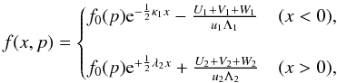 (3)where the downstream integral terms
U2, V2, and
W2 are given by:
(3)where the downstream integral terms
U2, V2, and
W2 are given by: 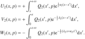 (4)In the upstream region,
U1, V1, and
W1 are still given by Eq. (4) after performing the substitutions 1 → 2,
κ2 → −λ1,
λ2 → −κ1, and ∞ → −∞. The
distribution function at the shock position, f0, is determined
by the matching conditions at x = 0. We integrate Eq. (1) in a thin region across the shock front.
Assuming that
D ≡ D1 = D2, we
find the equation for f0
(4)In the upstream region,
U1, V1, and
W1 are still given by Eq. (4) after performing the substitutions 1 → 2,
κ2 → −λ1,
λ2 → −κ1, and ∞ → −∞. The
distribution function at the shock position, f0, is determined
by the matching conditions at x = 0. We integrate Eq. (1) in a thin region across the shock front.
Assuming that
D ≡ D1 = D2, we
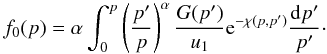
find the equation for f0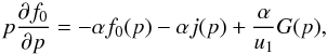 (5)where
α = 3u1/(u1 − u2)
is the known DSA spectral index. The term G denotes the sum of the
upstream and downstream source integrals
(5)where
α = 3u1/(u1 − u2)
is the known DSA spectral index. The term G denotes the sum of the
upstream and downstream source integrals
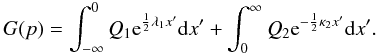 (6)The function
j(p) is linked to the destruction term
Γinel. It is defined as
(6)The function
j(p) is linked to the destruction term
Γinel. It is defined as 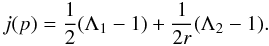 (7)After defining the function
 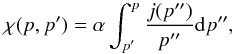 (8)the solution of Eq. (5) can be expressed in the simple form
 (9)From Eq. (3), one recovers the standard DSA solution by setting
Γinel = 0 (no interactions) and assuming that the injection occurs only at the
shock front
(Ui = Vi = Wi = 0):
one finds that f2 = f0 and
f1 = f0eu1x/D1,
while Eq. (9) gives a
spectrum p−α, provided that the source term
G(p) is softer than
p−α (see Sect. 2.4). Some simplifications can be made by analyzing the timescales of
the problem. The DSA acceleration rate for particles of momentum p in a
stationary shock is
(9)From Eq. (3), one recovers the standard DSA solution by setting
Γinel = 0 (no interactions) and assuming that the injection occurs only at the
shock front
(Ui = Vi = Wi = 0):
one finds that f2 = f0 and
f1 = f0eu1x/D1,
while Eq. (9) gives a
spectrum p−α, provided that the source term
G(p) is softer than
p−α (see Sect. 2.4). Some simplifications can be made by analyzing the timescales of
the problem. The DSA acceleration rate for particles of momentum p in a
stationary shock is  , where we assumed Bohm diffusion
(D ∝ p) and strong shocks (r ≈ 4).
For a SNR of age τsnr, the condition
, where we assumed Bohm diffusion
(D ∝ p) and strong shocks (r ≈ 4).
For a SNR of age τsnr, the condition
 defines the maximum momentum
pmax attainable by DSA. In the presence of hadronic
interactions, the requirement Γinel ≪ Γacc must be fulfilled. These
relations imply that
20 ΓinelD/u2 ≪ 1 and
xΓinel/u ≪ 1 at all the energies
considered. Under these conditions, we can linearly expand
Λ ≈ 1 + 2ΓinelD/u2, so that
λ ≈ 2Γinel/u and
κ ≈ 2u/D + 2Γinel/u.
The exponential terms of Eqs. (3) and
(4) can also be expanded as
defines the maximum momentum
pmax attainable by DSA. In the presence of hadronic
interactions, the requirement Γinel ≪ Γacc must be fulfilled. These
relations imply that
20 ΓinelD/u2 ≪ 1 and
xΓinel/u ≪ 1 at all the energies
considered. Under these conditions, we can linearly expand
Λ ≈ 1 + 2ΓinelD/u2, so that
λ ≈ 2Γinel/u and
κ ≈ 2u/D + 2Γinel/u.
The exponential terms of Eqs. (3) and
(4) can also be expanded as
 and
and
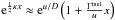 . Thus, the function
j(p) of Eq. (7) is given by
. Thus, the function
j(p) of Eq. (7) is given by 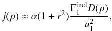 (10)and the integral of Eq. (8) by
 ![Mathematical equation: \begin{equation} \label{Eq::ChiApprox} \chi(p,p^{\prime}) \approx \alpha (1+r^{2}) \frac{\Gamma^{\rm inel}_{1}}{u_{1}^{2}} [ D(p) - D(p^{\prime}) ], \end{equation}](/articles/aa/full_html/2012/08/aa18967-12/aa18967-12-eq89.png) (11)which recovers the expression of Mertsch & Sarkar (2009). Below we present the DSA
solutions for primary nuclei (injected at the shock), their secondary fragments (generated
in the SNR environment), and pre-existing CR particles that undergo re-acceleration.
(11)which recovers the expression of Mertsch & Sarkar (2009). Below we present the DSA
solutions for primary nuclei (injected at the shock), their secondary fragments (generated
in the SNR environment), and pre-existing CR particles that undergo re-acceleration.
2.2. Acceleration of primary nuclei
The injection of ambient particles is assumed to occur immediately upstream from the
shock at momentum pinj. The source term for primary nuclei is
 (12)Particles can be injected only when their
Larmor radius is large enough to cross the shock thickness. Thus, we
assume a reference injection rigidity for all nuclei, Rinj, so
that
pinj = ZRinj. The
constant Y reflect the particle abundances in the ISM and their injection
efficiencies. In this work, they are determined by the data. The phase space density
profile is given by
(12)Particles can be injected only when their
Larmor radius is large enough to cross the shock thickness. Thus, we
assume a reference injection rigidity for all nuclei, Rinj, so
that
pinj = ZRinj. The
constant Y reflect the particle abundances in the ISM and their injection
efficiencies. In this work, they are determined by the data. The phase space density
profile is given by  (13)The upstream profile,
~eu1x/D,
indicates that the plasma is confined near the shock within a typical distance
~D/u1. Owing to advection, the
particles are accumulated in the downstream region, where destruction processes give rise
to the term
(13)The upstream profile,
~eu1x/D,
indicates that the plasma is confined near the shock within a typical distance
~D/u1. Owing to advection, the
particles are accumulated in the downstream region, where destruction processes give rise
to the term  . The momentum spectrum at the shock
position is
f0 ∝ e−χp−α,
which is the known DSA power-law behavior times an exponential factor,
~e−χ, given by
χ ≈ αΓinel/Γacc. The condition
. The momentum spectrum at the shock
position is
f0 ∝ e−χp−α,
which is the known DSA power-law behavior times an exponential factor,
~e−χ, given by
χ ≈ αΓinel/Γacc. The condition
 implies that χ ≲ 1.
2.3. Production and acceleration of secondary nuclei
Secondary nuclei originate in the SNR environment from the spallation of heavier nuclei
on the background medium. The source term for a j-type CR species arises
from the sum of all heavier k-type nuclei,
 . Each partial contribution is defined to
be:
. Each partial contribution is defined to
be:  (14)where
Nk(x, p′) = 4πp′2fk(x, p′)
is the progenitor number density and
(14)where
Nk(x, p′) = 4πp′2fk(x, p′)
is the progenitor number density and  is the
k → j fragmentation rate, which is implicitly summed
over the circumstellar abundances (the hydrogen and helium components). We have assumed
that the kinetic energy per nucleon is conserved in the process, i.e., the fragments are
ejected with momentum
ξkj = Aj/Ak
times smaller than that of their parents. The presence of short-lived isotopes
(ghost nuclei) such as 9Li or 11C is reabsorbed
in the definition of σkj, while long-lived
isotopes such as 10Be or 26Al (lifetime ~1 Myr) are considered
as stable during the acceleration process (timescale
τsnr ~10 kyr). The source spatial profile takes the form
of the progenitor nucleus of Eq. (13). In
the upstream region, one has
is the
k → j fragmentation rate, which is implicitly summed
over the circumstellar abundances (the hydrogen and helium components). We have assumed
that the kinetic energy per nucleon is conserved in the process, i.e., the fragments are
ejected with momentum
ξkj = Aj/Ak
times smaller than that of their parents. The presence of short-lived isotopes
(ghost nuclei) such as 9Li or 11C is reabsorbed
in the definition of σkj, while long-lived
isotopes such as 10Be or 26Al (lifetime ~1 Myr) are considered
as stable during the acceleration process (timescale
τsnr ~10 kyr). The source spatial profile takes the form
of the progenitor nucleus of Eq. (13). In
the upstream region, one has  , where
Dk is the diffusion coefficient of the
progenitor nucleus at the momentum
p/ξkj. For
D ∝ p/Z, one can write
Dk(p/ξkj) = ζkjDj(p),
where
, where
Dk is the diffusion coefficient of the
progenitor nucleus at the momentum
p/ξkj. For
D ∝ p/Z, one can write
Dk(p/ξkj) = ζkjDj(p),
where  . In practice,
ζkj ≈ 1 for all processes
k → j with
Zj,k > 2. The terms at the shock,
q1,jk and
q2,jk, are given by
. In practice,
ζkj ≈ 1 for all processes
k → j with
Zj,k > 2. The terms at the shock,
q1,jk and
q2,jk, are given by
 (15)and the downstream solution reads
![Mathematical equation: \begin{equation} \label{Eq::DownStreamSecondary} f_{2,j}(x,p) = f_{0,j}(p) + \left[ \frac{q_{2,j}(p)}{u_{2}}- \Gamma^{\rm frag}_{2,j}f_{0,j}(p) \right] x, \end{equation}](/articles/aa/full_html/2012/08/aa18967-12/aa18967-12-eq128.png) (16)where
f0,j is given from Eq. (9) using G(p)
by the expression
(16)where
f0,j is given from Eq. (9) using G(p)
by the expression  (17)We solve all equations starting from the
heaviest element and proceeding downward in mass. We are interested in the total
contribution of SNRs to the Galactic CR population, which we evaluate to be the integral
of the downstream solution over the SNR volume left behind the shock
(17)We solve all equations starting from the
heaviest element and proceeding downward in mass. We are interested in the total
contribution of SNRs to the Galactic CR population, which we evaluate to be the integral
of the downstream solution over the SNR volume left behind the shock  (18)where
xmax = u2τsnr
and ℛsnr is the supernovae explosion rate per unit volume in the Galaxy.
(18)where
xmax = u2τsnr
and ℛsnr is the supernovae explosion rate per unit volume in the Galaxy.
2.4. Re-acceleration of background CR nuclei
Together with the thermal ISM particles of Sect. 2.2, SNR shock waves may also accelerate the background CRs at equilibrium (Berezhko et al. 2003; Wandel et al. 1987). We refer to this mechanism as the re-acceleration
of CRs in SNRs. For a prescribed distribution function of background CRs,
 , the DSA solution at the shock is simply
 (19)Assuming, for illustrative purposes, a
power-law form
(19)Assuming, for illustrative purposes, a
power-law form  , the resulting re-acceleration spectrum is
![Mathematical equation: \begin{equation} f_{0,j}^{\rm re}(p) = \frac{\alpha}{\alpha-s} \left[ 1 - (p/p^{\rm inj}_{j})^{-\alpha + s} \right]f^{\rm bg}_{j}(p). \end{equation}](/articles/aa/full_html/2012/08/aa18967-12/aa18967-12-eq137.png) (20)Since the CR equilibrium spectrum,
fbg ∝ p−s, is
softer than the test-particle one (s > α), for
(20)Since the CR equilibrium spectrum,
fbg ∝ p−s, is
softer than the test-particle one (s > α), for
 one obtains
 (21)That is, the effect of re-acceleration is to
re-distribute the CR spectrum to p−α.
Interestingly, in the opposite case (s < α) the
re-accelerated spectrum maintains its spectral shape
p−s, while its normalization is amplified
by the factor α/(s − α). In our model,
however, the background spectrum fbg is computed as discussed
in Sect. 3 and takes the SNR spectra as input.
Therefore, Eq. (19) is an
integro-differential equation where the DSA-mechanism is fed by its DHM-propagated
solution and vice-versa. On the other hand, the bulk of the re-accelerated CRs come from
the low-energy part of the spectrum (below ~10 GV of rigidity), where the
equilibrium CR spectra are fixed by the observations so they cannot vary too much. It can
be safely assumed that re-accelerated CRs are a sub-dominant component of the total
(integral) flux. Hence, we proceed using an iterative method as outlined in Sect. 4.5.
(21)That is, the effect of re-acceleration is to
re-distribute the CR spectrum to p−α.
Interestingly, in the opposite case (s < α) the
re-accelerated spectrum maintains its spectral shape
p−s, while its normalization is amplified
by the factor α/(s − α). In our model,
however, the background spectrum fbg is computed as discussed
in Sect. 3 and takes the SNR spectra as input.
Therefore, Eq. (19) is an
integro-differential equation where the DSA-mechanism is fed by its DHM-propagated
solution and vice-versa. On the other hand, the bulk of the re-accelerated CRs come from
the low-energy part of the spectrum (below ~10 GV of rigidity), where the
equilibrium CR spectra are fixed by the observations so they cannot vary too much. It can
be safely assumed that re-accelerated CRs are a sub-dominant component of the total
(integral) flux. Hence, we proceed using an iterative method as outlined in Sect. 4.5.
 |
Fig. 1 Energy spectra of the CR elements Li, Be, B, C, N, O, Ne, Mg and Si. The solid lines represent the reference model prediction. The dashed lines indicate the secondary CR component arising by collisions of heavier nuclei in the ISM. The model parameters are listed in Table 1. Data are from HEAO3-C2 (Engelmann et al. 1990), CREAM (Ahn et al. 2009), AMS-01 (Aguilar et al. 2010), TRACER (Ave et al. 2008; Obermeier et al. 2011), ATIC-2 (Panov et al. 2009), CRN (Müller et al. 1991), Simon et al. (1980), Lezniak & Webber (1978) and Orth et al. (1978). The Li-Be-B data from CREAM and AMS-01 are combined with our model to obtain the spectra from their secondary-to-primary ratios. |
3. Interstellar propagation
We use a DHM to describe the CR transport and interactions in the ISM in a two-dimensional
geometry. We disregard the effects of energy losses, diffusive reacceleration, and
convection. The Galaxy is modeled as a disk of half-thickness h, containing
the gas and the CR sources. The disk is surrounded by a cylindrical diffusive halo of
half-thickness L, radius rmax, and zero matter
density. The CRs diffuse into both the disk and the halo. The diffusion coefficient is taken
to be rigidity dependent and position independent such that
K(R) = βK0(R/R0)δ.
The number density Nj of the nucleus
j is a function of the kinetic energy per nucleon, E,
and the position (r,z). The steady-state transport equation can be written
as  (22)The loss term,
 , describes the decay rate of unstable
nuclei,
, describes the decay rate of unstable
nuclei,  (where
γL is the usual Lorentz factor) and the
total destruction rate for collisions in the disk,
(where
γL is the usual Lorentz factor) and the
total destruction rate for collisions in the disk,  . The source term,
 , is the sum of contributions from SNRs
(the DSA solution of Eq. (18)), and the
secondary production in the ISM from k-type progenitors
, is the sum of contributions from SNRs
(the DSA solution of Eq. (18)), and the
secondary production in the ISM from k-type progenitors 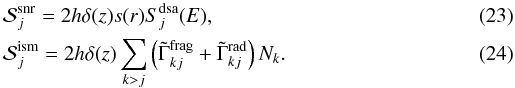 The function
s(r) expresses the SNR radial distribution in the disk,
that we assume to be uniform. For primary CRs, Sdsa is
normalized by the Y constants of Eq. (12). In our study, secondary nuclei may have a non-zero
Sdsa term. The term
The function
s(r) expresses the SNR radial distribution in the disk,
that we assume to be uniform. For primary CRs, Sdsa is
normalized by the Y constants of Eq. (12). In our study, secondary nuclei may have a non-zero
Sdsa term. The term  describe the contributions
k → j from unstable progenitors of lifetime
τkj. In Eq. (24),
describe the contributions
k → j from unstable progenitors of lifetime
τkj. In Eq. (24),  and
and  . The conditions
Nj ≡ 0 at the halo boundaries and the
continuity condition across the disk completely characterize the solution of Eq. (22). The full solution is reported in Maurin et al. (2001). We again solve the transport
equations for all the CR nuclei following their top–down fragmentation sequence, plus a
second iteration to account for the 10Be → 10B decay. The differential
fluxes as a function of kinetic energy per nucleon E are obtained from
. The conditions
Nj ≡ 0 at the halo boundaries and the
continuity condition across the disk completely characterize the solution of Eq. (22). The full solution is reported in Maurin et al. (2001). We again solve the transport
equations for all the CR nuclei following their top–down fragmentation sequence, plus a
second iteration to account for the 10Be → 10B decay. The differential
fluxes as a function of kinetic energy per nucleon E are obtained from
 (25)where the equilibrium solutions are computed at
the Solar System position (r,z) = (8.5 kpc,0). The basic DHM predictions
can be seen, for illustrative purpose, in the one-dimensional limit
rmax → ∞. The solution for a pure primary CR is given by
(25)where the equilibrium solutions are computed at
the Solar System position (r,z) = (8.5 kpc,0). The basic DHM predictions
can be seen, for illustrative purpose, in the one-dimensional limit
rmax → ∞. The solution for a pure primary CR is given by
 (26)where the spallation rate is neglected for
simplicity. The effect of the propagation in steepening the spectrum is clearly evident: for
a source spectrum
Sdsa(E) ∝ E−ν
and a Galactic diffusion coefficient of the type
K(E) ∝ Eδ,
the model predicts that
N(E) ∝ E−ν − δ.
To resolve the two parameters ν and δ, one has to consider
pure secondary species. The solution for a one-progenitor secondary CR is given by
Eq. (26), with the replacement of
Sdsa with
(26)where the spallation rate is neglected for
simplicity. The effect of the propagation in steepening the spectrum is clearly evident: for
a source spectrum
Sdsa(E) ∝ E−ν
and a Galactic diffusion coefficient of the type
K(E) ∝ Eδ,
the model predicts that
N(E) ∝ E−ν − δ.
To resolve the two parameters ν and δ, one has to consider
pure secondary species. The solution for a one-progenitor secondary CR is given by
Eq. (26), with the replacement of
Sdsa with  , so that the ratio
Ns/Np ∝ L/K
allows the simultaneous determination of δ and
K0/L. These simple trends are valid for the
reference model, i.e. when only primary CRs have a source term. In the
case of a secondary SNR component, depending on its intensities, the parameter determination
may be more complicated.
, so that the ratio
Ns/Np ∝ L/K
allows the simultaneous determination of δ and
K0/L. These simple trends are valid for the
reference model, i.e. when only primary CRs have a source term. In the
case of a secondary SNR component, depending on its intensities, the parameter determination
may be more complicated.
4. Analysis and results
We now review the model parameters and test the reference model setup. We then analyze the secondary CR production and re-acceleration in SNRs in some simple scenarios.
4.1. Model parameters
The DSA mechanism of Sect. 2 provides power-law
spectra
Sdsa ∝ E−ν with
a unique spectral index ν = α − 2 for all the primary
CRs, where α, in turn, is linked to the compression
ratio r, which is specified by δ and the observed
log-slope γ. To match γ ≈ 2.7 with
δ < 0.7, one has to adopt a compression factor of
r < 4, in contrast to the value r = 4 required for
strong shocks. Despite this tension between DSA and observations, we regard
r as an effective quantity describing the compression ratio actually
felt by the particles, which is not necessary related to the physical strength of the SNR
shocks (Ptuskin et al. 2010). The diffusion
coefficient around the shock is taken to be Bohm-like,
 . The ambient magnetic field
B may reach ~100 μG or more, because of
amplification effects, except for the very late SNR evolutionary stages, where the
magnetic field may be damped (B ≲ μG). In our
steady-state description, the SNR parameters have to be considered as effective
time-averaged quantities representing a more complex situation where the shock structure
evolves with time and may be influenced by the back-reaction of accelerated CRs. The
average shock speed u1 is of the order of
108 cm s-1. The upstream gas density,
n1, is poorly known and may well vary from
~10-3 to ~10 cm-3, depending on the SNR progenitor
star or its local environment. The SNR explosion rate per unit volume is expressed as a
surface density, 2hℛsnr, that we fix to
25 Myr-1 kpc-2 (Grenier
2000).
. The ambient magnetic field
B may reach ~100 μG or more, because of
amplification effects, except for the very late SNR evolutionary stages, where the
magnetic field may be damped (B ≲ μG). In our
steady-state description, the SNR parameters have to be considered as effective
time-averaged quantities representing a more complex situation where the shock structure
evolves with time and may be influenced by the back-reaction of accelerated CRs. The
average shock speed u1 is of the order of
108 cm s-1. The upstream gas density,
n1, is poorly known and may well vary from
~10-3 to ~10 cm-3, depending on the SNR progenitor
star or its local environment. The SNR explosion rate per unit volume is expressed as a
surface density, 2hℛsnr, that we fix to
25 Myr-1 kpc-2 (Grenier
2000).
The parameters describing the interstellar diffusion coefficient are fixed to δ = 0.5 and K0 = 0.089 kpc2 Myr-1 (see Sect. 4.2). Below the reference rigidity, R0 = 4 GV, we set δ = 0. However our analysis is always applied to rigidities R > R0. The halo radius is rmax = 20 kpc and its half-height is L = 5 kpc. As per the propagation in the ISM, the quantity that enters the model is surface density h × nism, where we take h = 0.1 kpc and nism = 1 cm-3. We assume a composition of 90% H + 10% He for the ISM gas density, nism, and that this composition, on average, is also found in the SNR background media. In addition, we include the solar modulation effect, though it is relevant only below few GeV nucleon-1. The modulation is described in the force-field approximation (Gleeson & Axford 1968) by means of the parameter φ, taken to be 500 MV, to characterize a medium-level modulation strength. Our nuclear chain starts with Zmax = 14 and processes all the relevant isotopes down to Z = 3. Nuclei with Z > 14 do not contribute significantly to the Li-Be-B abundances. The spallation cross-sections are taken from Silberberg et al. (1998). The cross-sections on He targets are obtained by means of the algorithm presented in Ferrando et al. (1998). The reference model parameters are listed in Table 1.
Source and transport parameter sets.
4.2. Reference model
Before analyzing the impact of SNR production and re-acceleration of secondary CRs on the parameter determination, we test the reference model predictions for the parameters in Table 1. Predictions at Earth for the CR elemental spectra Li, Be, B, C, N, O, Ne, Mg, and Si are presented in Fig. 1, where the total spectra (solid lines) are shown together their secondary component (dashed lines) arising from collisions in the ISM. The key quantities for propagation, K0 and δ, are determined from the B/C ratio above 2 GeV nucleon-1, using all the data reported in the past two decades, i.e., from the space-based experiments HEAO3-C2 (Engelmann et al. 1990), CRN (Swordy et al. 1990), and AMS-01 (Aguilar et al. 2010), and the balloon-borne projects CREAM (Ahn et al. 2009) and ATIC-2 (Panov et al. 2007). The primary nuclei spectra were normalized using data from CREAM (for C, N, O, Ne, Mg, and Si) and HEAO3-C2 (for all elements). Given the K0 − L degeneracy (see Sect. 3), in the following we adopt the quantity K0/L as the physical parameter, where the halo height L is fixed at 5 kpc.
As apparent from the figure, the reference model calculations give a good description of the CR elemental spectra within the precision of the present data. We note that, under this pure diffusion model, the B/C data between ~10 GeV and ~1 TeV per nucleon suggest that δ ~ 0.4, while the data at lower energies (~1–100 GeV nucleon-1) favor higher values (δ ~ 0.6). These uncertainties are related on both the model unknowns at ~GeV/n energies and the lack of data at ≳100 GeV nucleon-1 (Maurin et al. 2010). We also note that the reference model predictions are insensitive to the source parameters n1, u1, and B: the source spectra are specified only by the effective compression ratio r (via γ and δ) and the abundance constants Y. This setup is equivalent to that of many diffusion models, e.g. Maurin et al. (2001), that make use of rigidity power-law parameterizations as source functions.
4.3. SNR models
Similarly to Morlino (2011), we consider two ideal situations represented by Type I/a (important for fragmentation, Sect. 4.4) and core-collapse supernovae (important for re-acceleration, Sect. 4.5). In the Type I/a scenario, the supernova explodes in the regular ISM with typical density and temperature n1 ≈ 1 cm-3 and T0 = 104 K. In the core-collapse scenario, the SNR expands into a hot diluted bubble (n1 ≪ 1 cm-3 and T0 ≫ 104 K) that may be generated by either the progenitor’s wind or by previous SNR explosions that occurred in the same region. In both scenarios, the circumstellar densities are assumed to be homogeneous and constant during the SNR evolution. Two SNR evolutionary stages are relevant to our study: the ejecta-dominated (ED) phase, when the shock front expands freely and accumulates the swept-up mass in the SNR interior, and the Sedov-Taylor (ST) expansion phase, which is driven by the thermal pressure of the hot gas. The phase transition ED–ST occurs at the time τst, when the swept-up mass equals the mass of the ejecta Mej. The CR acceleration ceases at the time τsnr.
Case studies of Type I/a and core-collapse SNRs.
For all the models, we assume Esnr = 5 × 1051 erg,
Mej = 4 M⊙, and
τsnr = 20 kyr, where Esnr is the
SNR explosion energy (not converted into neutrinos) and M⊙ is
the solar mass. The cases of different τsnr values are
considered in Sect. 4.6. During the ED stage, the
SNR radius grows with a constant rate
Rsh(t) = u1t,
at the speed
u1 = (2Esnr/Mej)1/2 ~ 108 cm s-1,
until it reaches the swept-up radius
Rsw ≡ Rsh(τst).
For a given SNR model characterized by n1 and
τsnr, we parametrize the shock evolution
(Rsh and u1) using the
self-similar solutions derived in Truelove & McKee
(1999) for a remnant expanding into a homogeneous medium. These solutions connect
smoothly the ED phase (Rsh ∝ t) with the ST
stage (Rsh ∝ t2/5). The CR
acceleration ceases at time τsnr, from which we compute the
average velocity  . Thus, we use
 as an input parameter for our steady-state
DSA calculations (Sect. 2.1) to compute the spectra
for all the CR elements. The SNR models considered are listed in Table 2.
as an input parameter for our steady-state
DSA calculations (Sect. 2.1) to compute the spectra
for all the CR elements. The SNR models considered are listed in Table 2.
We always assume that the total CR flux is produced by SNRs of only one type: for each SNR model, the parameters employed have to be regarded as effective ones representing the average population of CR sources. We note that this simplified breakdown is somewhat artificial, because the total CR flux may be due to a complex ensemble of contributing SNRs.
4.4. Secondary CR production in Type I/a SNRs
The secondary production of CRs is relevant for SNRs that expand into ambient densities of the order of n1 ~ 1 cm-3, where the quantity n1 represents the average SNR background density. Such a value may be higher than that of the average ISM, owing to, e.g., contributions from SNRs located in high density regions of the Galactic bulge, inside the dense cores of molecular clouds or SNRs expanding into the winds of their progenitors.
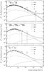 |
Fig. 2 Energy spectra of secondary elements Li, Be, and B. The source components from
fragmentation occurring inside SNRs are split into the
|
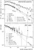 |
Fig. 3 Top: individual CR spectra of B and C. Solid lines are the model predictions for I/a #3 SNR model of Table 2. Model parameters are as in Table 1, except for δ and K0/L, which are fitted to data. The boron SNR component (dotted line) and the ISM component (dashed lines) are reported. Bottom: the B/C ratio from the above model (solid line) and when fragmentation in SNR is turned off (dashed line). Data are from HEAO3-C2 (Engelmann et al. 1990), CREAM (Ahn et al. 2009), AMS-01 (Aguilar et al. 2010), TRACER (Obermeier et al. 2011), ATIC-2 (Panov et al. 2007), CRN (Müller et al. 1991), Simon et al. (1980), Lezniak & Webber (1978), and Orth et al. (1978). |
From Eq. (16), one sees that the
secondary CR flux emitted by SNRs has two components. By analogy with Blasi & Serpico (2009) and Kachelrieß et al. (2011), these are referred to as
 and ℬ. The -term,
proportional to f0, describes the particles that are produced
within a distance ~D/u of both the sides of the
shock front and are still able to undergo DSA. From Eq. (17), the -spectrum
is f ~ p−α + 1,
reflecting the spectrum of their progenitors
(f ~ p−α) and the
momentum dependence of the diffusion coefficient, D ∝ p.
The ℬ-term, f ~ q2, describes those
secondary nuclei that, after being produced, are simply advected downstream without
experiencing further acceleration. Their spectrum maintains the same behavior as that of
their progenitors
q2 ~ p−α.
These components are illustrated in Fig. 2 for the
spectra at Earth of Li, Be, and B for a SNR with
n1 = 2 cm-3,
u1 = 5 × 107 cm s-1, and
B = 0.1 μG. The figure compares the standard ISM
components (solid lines) with the source components
(short-dashed lines) and ℬ (long-dashed lines) within the same propagation parameter set.
Both the source components are harder than those expected from the standard CR production
in ISM; in particular, the -term
leads to increasing secondary-to-primary ratios at high energies (Blasi 2009; Mertsch & Sarkar
2009). While the ℬ-term depends on the SNR ambient
density n1 and its age τsnr, the
-term
also relies on the diffusion properties, as its strength is proportional to
~
and ℬ. The -term,
proportional to f0, describes the particles that are produced
within a distance ~D/u of both the sides of the
shock front and are still able to undergo DSA. From Eq. (17), the -spectrum
is f ~ p−α + 1,
reflecting the spectrum of their progenitors
(f ~ p−α) and the
momentum dependence of the diffusion coefficient, D ∝ p.
The ℬ-term, f ~ q2, describes those
secondary nuclei that, after being produced, are simply advected downstream without
experiencing further acceleration. Their spectrum maintains the same behavior as that of
their progenitors
q2 ~ p−α.
These components are illustrated in Fig. 2 for the
spectra at Earth of Li, Be, and B for a SNR with
n1 = 2 cm-3,
u1 = 5 × 107 cm s-1, and
B = 0.1 μG. The figure compares the standard ISM
components (solid lines) with the source components
(short-dashed lines) and ℬ (long-dashed lines) within the same propagation parameter set.
Both the source components are harder than those expected from the standard CR production
in ISM; in particular, the -term
leads to increasing secondary-to-primary ratios at high energies (Blasi 2009; Mertsch & Sarkar
2009). While the ℬ-term depends on the SNR ambient
density n1 and its age τsnr, the
-term
also relies on the diffusion properties, as its strength is proportional to
~ . However, the parameter combination
 should be sufficiently large to ensure an
-term
dominance at ~TeV energies, which can be realized only in the latest evolutionary
stage of a SNR characterized by damped magnetic fields
(B ≪ 1 μG) and low shock speeds
(u1 < 108 cm s-1). On the other
hand, the local flux of stable CR nuclei depends on the large-scale structure of the
galaxy (of some kpc) and reflects the contribution of a relatively large population of
SNRs and their histories (Taillet & Maurin
2003). Furthermore, from Eqs. (9)
and (11), the
-term
induces an exponential cut-off at momentum pcut given by
χ(pcut) ≈ 1, which is not observed in
present data of primary or secondary CR spectra. Since our aim is to estimate these
effects when the considered SNRs produce all the observed CR flux, the associated
parameters have to be able to accelerate all CR nuclei up to, say,
pmax/Z ~ 106 GV. Thus, from
the requirement that χ ≲ 1 for any p up to
pmax (see Sect. 2.1),
the -term
is always ineffective at the energies we consider and is not discussed below. Given the
absence of a clear spectral feature in the ℬ-term, the spectral deformation induced by
interactions in SNRs may be difficult to detected ~TeV energies, because it can be
easily mimicked by a different choice of δ and
K0/L. This is illustrated in Fig. 3, where the total boron spectrum (solid line) is plotted
showing its standard component arising from ISM collisions (dashed line) and the source
component coming from hadronic interactions in SNRs (dotted line). The SNR model is the
I/a #3 of Table 2. We note that the carbon flux
also contains a small amount of secondary fragments (≲ 5%), produced in both ISM and SNRs.
The B/C ratio is also plotted for the reference model (dashed line) under
the same propagation parameter setting, i.e. when hadronic interactions in SNRs are turned
off. The effect of including secondary production in the sources translates into a slight
increase at 100 GeV nucleon-1, while it reaches a factor 2.5 at 1 TeV
nucleon-1 and one order of magnitude at 10 TeV nucleon-1.
should be sufficiently large to ensure an
-term
dominance at ~TeV energies, which can be realized only in the latest evolutionary
stage of a SNR characterized by damped magnetic fields
(B ≪ 1 μG) and low shock speeds
(u1 < 108 cm s-1). On the other
hand, the local flux of stable CR nuclei depends on the large-scale structure of the
galaxy (of some kpc) and reflects the contribution of a relatively large population of
SNRs and their histories (Taillet & Maurin
2003). Furthermore, from Eqs. (9)
and (11), the
-term
induces an exponential cut-off at momentum pcut given by
χ(pcut) ≈ 1, which is not observed in
present data of primary or secondary CR spectra. Since our aim is to estimate these
effects when the considered SNRs produce all the observed CR flux, the associated
parameters have to be able to accelerate all CR nuclei up to, say,
pmax/Z ~ 106 GV. Thus, from
the requirement that χ ≲ 1 for any p up to
pmax (see Sect. 2.1),
the -term
is always ineffective at the energies we consider and is not discussed below. Given the
absence of a clear spectral feature in the ℬ-term, the spectral deformation induced by
interactions in SNRs may be difficult to detected ~TeV energies, because it can be
easily mimicked by a different choice of δ and
K0/L. This is illustrated in Fig. 3, where the total boron spectrum (solid line) is plotted
showing its standard component arising from ISM collisions (dashed line) and the source
component coming from hadronic interactions in SNRs (dotted line). The SNR model is the
I/a #3 of Table 2. We note that the carbon flux
also contains a small amount of secondary fragments (≲ 5%), produced in both ISM and SNRs.
The B/C ratio is also plotted for the reference model (dashed line) under
the same propagation parameter setting, i.e. when hadronic interactions in SNRs are turned
off. The effect of including secondary production in the sources translates into a slight
increase at 100 GeV nucleon-1, while it reaches a factor 2.5 at 1 TeV
nucleon-1 and one order of magnitude at 10 TeV nucleon-1.
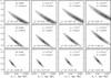 |
Fig. 4 Fit results for the parameters δ and K0/L of our models with fragmentation in Type I/a SNRs. Results are shown for Emin = 2, 5 and 10 GeV nucleon-1 (top to bottom), for the reference model and for the SNR models I/a # 1, # 2 and # 3 (left to right) of Table 2. The shaded areas represent the 1-, 2- and 3-σ contour limits. The markers “ × ” indicate the best-fit parameters for each configuration; the χ2/d.f. ratio is reported in each panel. |
From the B/C ratio data, we determined the parameters K0/L and δ for the Type I/a SNR models of Table 2. We performed a χ2 analysis using our model interfaced with MINUIT. The data were fit above a minimal energy of Emin = 10 GeV nucleon-1, as a compromise between the diffusion–dominated regime and the availability of experimental data. We also repeated the fits down to lower Emin to test the relevance of low energy effects to our model. The results are shown in Fig. 4 for Emin = 2, 5, and 10 GeV nucleon-1 (from top to bottom), for reference model and I/a models of Table 2 (left to right). The shaded areas represent the 1-, 2-, and 3-σ contour limits of the χ2. We stress that these parameter uncertainties are those arising from the fits and that they are contextual to our models. Owing to the complexity of the physics processes involved together with the possible lack of knowledge of several astrophysical inputs, the actual parameter uncertainties may be much larger (Maurin et al. 2010). For instance, the published values of δ vary widely from ~0.3 to ~0.7. The markers describe the best-fit parameters for each configuration. The χ2 values reported in each panels are divided by the degrees of freedom d.f. = 26, 21, and 16 for the considered energy thresholds. It can be seen from Fig. 4 that the source component has a little effect for model I/a #3 (n1 = 0.5 cm-3). When denser media were considered, the secondary source component was found to flatten the B/C ratio, so that higher values of δ were required to match the data. This trend is clearly apparent in Fig. 4 (from left to right). Similar conclusions, though weaker, can be drawn for the K0/L parameter ratio. To first approximation, B/C ∝ L/K0, so that the presence of a SNR component of boron requires a larger K0/L ratio to match the data.
In summary, for the SNR models considered, the fragmentation in SNRs affects the parameter δ of ~5–15% (and K0/L of ~2–10%), but these models cannot be discriminated by present data because of the large uncertainties in the data. This n1–δ degeneracy is apparent by the χ2/d.f.-values, which are almost insensitive to the SNR properties.
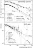 |
Fig. 5 Top: individual CR spectra of B and C. Solid lines are the model predictions for CC #2 SNR model of Table 2. Model parameters are as in Table 1 except for δ and K0/L, which are fitted to data. The boron SNR component (dotted line) and the ISM component (dashed lines) are reported. Bottom: the B/C ratio from the above model (solid line) and when re-acceleration is turned off (dashed line). Data as in Fig. 3. |
4.5. Re-acceleration in core-collapse SNRs
The amount of re-accelerated CRs depends on the total volume occupied by the SNRs (per
unit time) and their explosion rate (per unit volume). The fraction of re-accelerated CRs
to the total background CRs can be roughly estimated as
Nre/Nbg ~ Vsnrℛsnrτesc,
where Vsnr is the SNR volume and
τesc is the characteristic escape time of CRs in the Galaxy.
At a few GeV nucleon-1,
τesc ~ 2hL/K ~ 5 Myr.
The Vsnr is mainly determined by its expansion during the ED
phase; the SNR reaches a spherical volume  ,
where
,
where  is the mean mass of the ambient gas. Thus
Nre/Nbg ∝ 1/n1,
which is an opposite trend to that of the fragmentation scenario of Sect. 4.4. One can see that for a density
n1 ~ 1 cm-3 the re-acceleration gives a
small contribution to the total CR flux. In contrast, for
n1 ≲ 0.01 cm-3, the re-acceleration fraction
grows significantly (≳few percent). However it is also important the subsequent ST phase,
where the SNR shock expands adiabatically as
Rsh(t) ∝ t2/5,
slowing down at the rate
u1(t) = t−3/5.
is the mean mass of the ambient gas. Thus
Nre/Nbg ∝ 1/n1,
which is an opposite trend to that of the fragmentation scenario of Sect. 4.4. One can see that for a density
n1 ~ 1 cm-3 the re-acceleration gives a
small contribution to the total CR flux. In contrast, for
n1 ≲ 0.01 cm-3, the re-acceleration fraction
grows significantly (≳few percent). However it is also important the subsequent ST phase,
where the SNR shock expands adiabatically as
Rsh(t) ∝ t2/5,
slowing down at the rate
u1(t) = t−3/5.
Using the SNR parameters of Table 2, we computed
the re-accelerated CR spectra as in Sect. 2.2, using
Qreac = fbg(p)δ(x),
where  . Since CRs are already supra-thermal, we
assumed that all CR particles above pinj are suitable for
(re-)undergoing DSA. We note that N(p) is the DHM
solution of Eq. (22) that, in turn, is fed
by the total DSA spectra. Hence, we solved the DSA and DHM equation systems iteratively.
At the first iteration, only the standard injection term was considered (Eq. (12)) to compute the interstellar flux
N for all CR nuclei. The subsequent iterations made use of the previous
DHM solutions, N, to update the terms Qpri
and Qreac and to re-compute the total interstellar fluxes. The
procedure was iterated until the convergence was reached. At each iteration, the injection
constants, Y, were re-adjusted. The resulting CR flux (standard plus
re-accelerated) was therefore determined by Eq. (18) and is fully specified by the source parameters
n1 and τsnr. In practice, we
found that five iterations ensure a stable solution. The effect of re-acceleration is
shown in Fig. 5 for the SNR model CC #2 of
Table 2. At energies of
~1 TeV nucleon-1, the re-accelerated component dominates over the
ISM-induced component for secondary nuclei. It should be noted that the sources of
re-accelerated CRs may have a complex spatial distribution depending on the SNR spatial
profile. In our model, we used a uniform distribution,
s(r) ≡ 1, which does not limit the predicting power
of diffusion models as long as the key parameters are regarded as effective quantities
tuned to agree with the data (Maurin et al. 2001).
However, further elaborations would require more refined descriptions. In Fig. 6, we plot the fit results for the parameters
δ and K0/L for the
core-collapse SNR models of Table 2 and the
reference model. Compared to the scenario of Sect. 4.4, the results are less trivial to interpret because the background
CR flux that is subjected to re-acceleration itself depends on the parameters
δ and K0/L. As consequence
of this non-linearity, the K0/L best-fit
values results are less sensitive to n1. The results for
δ are qualitatively similar to those of Sect. 4.4, showing an opposite dependence on n1.
For the SNR model CC # 1 (n1 = 0.003 cm-3, left
column), the source component dominates the secondary CR flux at
~100 GeV nucleon-1, so that, at higher energies, the B/C ratio becomes
appreciably flat. The effect becomes less significant for higher background densities,
e.g., CC # 1 (n1 = 0.1 cm-3, right column) where
the best-fit parameters are close to those arising from the reference model
fit. As for the scenario of Sect. 4.4,
results are limited by the sizable uncertainties in the parameters that preclude
quantitative conclusions for
Emin = 10 GeV nucleon-1. Nonetheless, the figure
shows clear trends, especially for δ. The
χ2/d.f. values reported in each panel indicates that good fits
can be made for all the considered configurations, though they do not vary significantly
among the various SNR models.
. Since CRs are already supra-thermal, we
assumed that all CR particles above pinj are suitable for
(re-)undergoing DSA. We note that N(p) is the DHM
solution of Eq. (22) that, in turn, is fed
by the total DSA spectra. Hence, we solved the DSA and DHM equation systems iteratively.
At the first iteration, only the standard injection term was considered (Eq. (12)) to compute the interstellar flux
N for all CR nuclei. The subsequent iterations made use of the previous
DHM solutions, N, to update the terms Qpri
and Qreac and to re-compute the total interstellar fluxes. The
procedure was iterated until the convergence was reached. At each iteration, the injection
constants, Y, were re-adjusted. The resulting CR flux (standard plus
re-accelerated) was therefore determined by Eq. (18) and is fully specified by the source parameters
n1 and τsnr. In practice, we
found that five iterations ensure a stable solution. The effect of re-acceleration is
shown in Fig. 5 for the SNR model CC #2 of
Table 2. At energies of
~1 TeV nucleon-1, the re-accelerated component dominates over the
ISM-induced component for secondary nuclei. It should be noted that the sources of
re-accelerated CRs may have a complex spatial distribution depending on the SNR spatial
profile. In our model, we used a uniform distribution,
s(r) ≡ 1, which does not limit the predicting power
of diffusion models as long as the key parameters are regarded as effective quantities
tuned to agree with the data (Maurin et al. 2001).
However, further elaborations would require more refined descriptions. In Fig. 6, we plot the fit results for the parameters
δ and K0/L for the
core-collapse SNR models of Table 2 and the
reference model. Compared to the scenario of Sect. 4.4, the results are less trivial to interpret because the background
CR flux that is subjected to re-acceleration itself depends on the parameters
δ and K0/L. As consequence
of this non-linearity, the K0/L best-fit
values results are less sensitive to n1. The results for
δ are qualitatively similar to those of Sect. 4.4, showing an opposite dependence on n1.
For the SNR model CC # 1 (n1 = 0.003 cm-3, left
column), the source component dominates the secondary CR flux at
~100 GeV nucleon-1, so that, at higher energies, the B/C ratio becomes
appreciably flat. The effect becomes less significant for higher background densities,
e.g., CC # 1 (n1 = 0.1 cm-3, right column) where
the best-fit parameters are close to those arising from the reference model
fit. As for the scenario of Sect. 4.4,
results are limited by the sizable uncertainties in the parameters that preclude
quantitative conclusions for
Emin = 10 GeV nucleon-1. Nonetheless, the figure
shows clear trends, especially for δ. The
χ2/d.f. values reported in each panel indicates that good fits
can be made for all the considered configurations, though they do not vary significantly
among the various SNR models.
4.6. Summary and discussion
Our breakdown into Type I/a and core-collapse SNR scenarios is motivated by the complementary dependence of the two effects on n1. As seen in Sects. 4.4 and 4.5, the CR re-acceleration is found to be important for SNRs exploding into rarefied media, which are typical of super-bubbles (including our own local bubble), while the secondary production in SNRs is relevant for ambient densities similar to those of the regular ISM. Our calculations of the B/C ratio are in substantial agreement with the work of Berezhko et al. (2003) in the cases where the comparison can be made, though those authors used different approaches to model the acceleration as well as the interstellar propagation. The fit results for the SNR models of Table 2 and the reference model are listed in Table 3.
Figure 7 summarizes our findings, showing the best-fit parameters as functions of the SNR circumstellar density. The panel groups (a), (b), and (c) are referred to fits performed at different minimal energies, Emin = 10, 5, and 2 GeV nucleon-1, respectively. For each group, we report δ, K0/L, and χ2/d.f. as functions of n1 (from bottom to top, solid lines). The two mechanisms are presented separately: the sub-panels on the left-hand side show the effect of re-acceleration in CC type SNRs, while the right-hand side plots are referred to the secondary production by spallations in Type I/a SNRs. The complementarity of the two effects is apparent from the figure. In the region where they overlap, n1 ≈ 0.5 cm-3, neither is relevant. The horizontal (dotted) lines indicate the best-fit parameters for the reference model. Their dependence on Emin resembles that found in Di Bernardo et al. (2010), who also considered diffusive reacceleration models, although we note that we used a different set of data for the parameter determination. As discussed, the reference model is insensitive to either n1 or other SNR parameters. The dashed lines indicate the parameter uncertainties (at one σ of CL) arising from the fits.
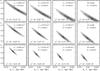 |
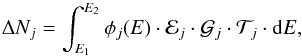
Fig. 6 Fit results for the parameters δ and K0/L of our models with re-acceleration in core-collapse SNRs. Results are shown for Emin = 2, 5, and 10 GeV nucleon-1 (top to bottom), for the SNR models CC # 1, # 2, and # 3 of Table 2 and for the reference model (left to right). The shaded areas represent the 1-, 2-, and 3-σ contour limits. The markers “ × ” indicate the best-fit parameters for each configuration; the χ2/d.f. ratio is reported in each panel. |
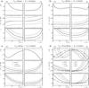 |
Fig. 7 Best-fit parameters δ and K0/L and the corresponding χ2/d.f. as function of n1 (solid lines) for models with re-acceleration in core-collapse SNRs (CC, left sub-panels) and with hadronic interactions in Type I/a SNRs (I/a, right sub-panels). The panel groups a), b) and c) show the fit results for data at Emin = 1, 10, 5, and 2 GeV nucleon-1, respectively, for τsnr = 20 kyr. Panel d) shows the results for τsnr = 10, 20, 40, 60, and 80 kyr in the case of Emin = 2 GeV nucleon-1. The horizontal dotted lines indicate the reference model parameters. |
It is interesting to note the evolution of the best-χ2 structures when the minimal energy Emin is decreased from 10 GeV nucleon-1 (Fig. 7a) to 2 GeV nucleon-1 (Fig. 7c). When the low-energy B/C data are included in the fits, the χ2/d.f. distribution exhibits two minima. The B/C ratio data at low energies favor a slope (δ ~ 0.6), which is somewhat steeper than that observed in high energy data (δ ~ 0.4): these two regimes are matched by models of SNRs that emit secondary nuclei. In some previous studies, e.g. Trotta et al. (2011), it has been found that the secondary-to-primary ratios can be reproduced well at all energies using δ = 1/3 and a strong diffusive reacceleration (the interstellar Alfvénic speed is of the order of ~30 km s-1). However, this cannot be satisfactorily reconciled with the use of pure power-law functions for the CR sources. On the other hand, the trends we observe suggest a possible role of SNR-fragmentation or re-acceleration in reconciling the low-energy B/C data with those at higher energies in a pure diffusion scenario.
As we have stressed, the physical effects discussed in this work should be tested at high energies, where most of the complexity of the low-energy CR propagation can be neglected. Owing to the scarcity of CR data above 10 GeV nucleon-1, the parameter constraints reported in Fig. 7a do not allow us to make any firm discrimination among the different SNR models. However, the main trends are apparent. On the propagation side, all the non-standard scenarios point toward larger values for δ, which is in some tensions with the predictions for the interstellar turbulence (Strong et al. 2007) and with CR anisotropy studies (Ptuskin et al. 2006). On the acceleration side, large values of δ reduce the source spectral index closer to the value ν = 2, which is favored by the DSA theory for strong shocks.
In all these scenarios, the acceleration ceases at
τsnr = 20 kyr, which may not be the case given their
different SNR evolutionary properties. For instance, since the ST phase duration scales as
 (Truelove
& McKee 1999), one may expect core-collapse SNRs to have longer
τsnr than Type I/a SNRs. However, the parameter
τsnr represents the time for which the SNR is active as a CR
factory and it can be extremely difficult to estimate. Thus, in Fig. 7d, we give the fit results for different values of
τsnr from 10 kyr to 80 kyr
(Emin = 2 GeV nucleon-1). The effect of using
different τsnr is clear. The longer the time for which the SNR
is active, the larger the fragments produced in its interior. In practice, the secondary
CRs production in Type I/a SNRs is characterized by the product
n1τsnr. For re-acceleration, a
longer lifetime allows the SNR to occupy larger volumes. To first approximation, the
intensity of re-accelerated nuclei increases as
~τsnr/n1. As shown in the
figure, for longer values of τsnr, the re-acceleration effect
also becomes important for relatively high density media.
(Truelove
& McKee 1999), one may expect core-collapse SNRs to have longer
τsnr than Type I/a SNRs. However, the parameter
τsnr represents the time for which the SNR is active as a CR
factory and it can be extremely difficult to estimate. Thus, in Fig. 7d, we give the fit results for different values of
τsnr from 10 kyr to 80 kyr
(Emin = 2 GeV nucleon-1). The effect of using
different τsnr is clear. The longer the time for which the SNR
is active, the larger the fragments produced in its interior. In practice, the secondary
CRs production in Type I/a SNRs is characterized by the product
n1τsnr. For re-acceleration, a
longer lifetime allows the SNR to occupy larger volumes. To first approximation, the
intensity of re-accelerated nuclei increases as
~τsnr/n1. As shown in the
figure, for longer values of τsnr, the re-acceleration effect
also becomes important for relatively high density media.
5. The projected AMS-02 sensitivity
We switch now to some estimations for the AMS experiment1, which is devoted to direct measurements of Galactic CRs across a wide range of energy.
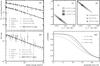 |
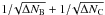
Fig. 8 AMS-02 mock data for the elemental fluxes φB and φCa) and their ratio b), using the input model CC # 2 of Table 2 and assuming a detector exposure factor F = 150 m2 sr day. The error bars are only statistics. The constraints to the transport parameters provided by the AMS-02 mock data are reported by the 3-σ contour levels for exposure factors of F = 12, 36, and 150 m2 sr day in c) and d). The data are fitted within the reference model (star in panel c) and dotted line in panel b)) and within the model CC # 2 (cross in panel d) and solid line in panel b)). The AMS-02 discrimination probability between the two models as a function of the systematic error in the measurement is shown in d) for F = 12, 36, and 150 m2 sr day. The systematic errors are assumed to be energy-independent. |
The prime goals of the AMS project are the direct search for anti-nuclei and the indirect search for dark matter particles. The first version of the experiment, AMS-01, operated in a test flight on June 1998. The final version of experiment, AMS-02, was successfully installed in the International Space Station on May 2011 and will be active for at least ten years. AMS-02 is able to identify CR elements from Z = 1 to Z = 26 and to determine their energy spectra from ~0.5 GeV to ~1 TeV per nucleon with unprecedented accuracy. We estimate the AMS-02 capabilities in determining the CR propagation properties for the considered scenarios.
5.1. Projected data
The AMS-02 sensitivity to CR nuclei measurements is studied by the generation of
mock data for a given input model. The number of
j-type particles recorded by AMS-02 at the kinetic energies between
E1 and E2 is given by
 (27)where
φj is the input spectrum,
(27)where
φj is the input spectrum,
 is the detector geometric factor, ℰj is the detection
efficiency, and
is the detector geometric factor, ℰj is the detection
efficiency, and  is the exposure time. All of these quantities are in general energy-dependent and
particle-dependent. The relevant quantity for our estimates is the exposure factor
is the exposure time. All of these quantities are in general energy-dependent and
particle-dependent. The relevant quantity for our estimates is the exposure factor
 ,
which we assume to be both energy and particle independent. We consider the cases of
ℱ = 12, 36, and 150 m2 sr day. For values of, e.g.,
,
which we assume to be both energy and particle independent. We consider the cases of
ℱ = 12, 36, and 150 m2 sr day. For values of, e.g.,
 0.45 m2 sr
and ℰ = 90%, our choices correspond to one month, three months and one year of time
exposures, respectively. We adopt a log-energy binning using nine bins per decade
between 10 GeV and 1 TeV per nucleon. The AMS-02 mock data for the B and C fluxes and
their ratios are shown in Figs. 8a and b. The
CR fluxes, φB and
φC, are calculated using the SNR model
CC # 2 (Table 2) as an input model. This “true”
model is characterized by the SNR parameters
n1 = 0.01 cm-3 and
τsnr = 20 kyr, and transport parameters
K0/L = 0.01847 kpc Myr-1 and
δ = 0.57. From Eq. (27), we compute the statistical error in each B/C data point as
0.45 m2 sr
and ℰ = 90%, our choices correspond to one month, three months and one year of time
exposures, respectively. We adopt a log-energy binning using nine bins per decade
between 10 GeV and 1 TeV per nucleon. The AMS-02 mock data for the B and C fluxes and
their ratios are shown in Figs. 8a and b. The
CR fluxes, φB and
φC, are calculated using the SNR model
CC # 2 (Table 2) as an input model. This “true”
model is characterized by the SNR parameters
n1 = 0.01 cm-3 and
τsnr = 20 kyr, and transport parameters
K0/L = 0.01847 kpc Myr-1 and
δ = 0.57. From Eq. (27), we compute the statistical error in each B/C data point as
 . Nonetheless, CR measurements are also
affected by systematic errors, which become increasingly important as the precision
increases with the collected statistics.
. Nonetheless, CR measurements are also
affected by systematic errors, which become increasingly important as the precision
increases with the collected statistics.
5.2. Discrimination power
We fit the B/C ratio mock data leaving K0/L and δ as free parameters. These parameters are determined within both the reference model (re-acceleration off) and the “true” re-acceleration model CC # 2 of Table 2. As shown in Fig. 8b, both the models can be tuned to reproduce the AMS-02 mock data, but they exhibit different functional shapes and deviate at high energies. The contour plots in panels (c) and (d) correspond to the best-fit parameters of the two models. Contour levels are shown for 3-σ uncertainty levels corresponding to the three exposure factors ℱ. As expected, the re-acceleration model fit (d) returns the correct parameters, while the reference model fit (c) misestimates the parameters because of inaccurate assumptions about the source properties. In fact, when the reference model is forced to describe the data, the spectral distortion induced by the re-acceleration is mimicked by the use of a lower value for δ. Given the precision of the AMS-02 data, this represents the dominant “error” in the parameter determination. As apparent from the figure, the AMS-02 data place tight constraints on the propagation parameters. For instance, δ is determined to a precision better than ≲10% within a 3–σ uncertainty level. The δ–n1 degeneracy may be lifted as in Castellina & Donato (2005), i.e., by a statistical test to discriminate between the two fits. As long as only statistical errors are considered, we find that the discrimination between the two scenarios is always possible for the three considered exposures at 90% of CL. The effect of systematic errors in the data is shown in Fig. 8e, where we plot the AMS-02 discrimination probability versus the relative systematic error. Our calculation assumes constant systematic errors (added in quadrature to the statistical ones), but these considerations also hold for energy-dependent systematic errors if their energy rise is less pronounced than the statistical errors. The solid, dashed, and dotted lines represent the cases of ℱ = 12, 36, and 150 m2 sr day, respectively. To achieve a discrimination of 90% CL, the systematic error has to be smaller than ~4%, 8%, and 10% for the three considered exposures. A 95% CL requirement also needs ℱ to be larger than 12 m2 sr day. We consider these requirements as reasonable for AMS-02, because the measurements of elemental ratios are only mildly sensitive to systematic errors.
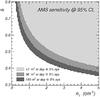 |
Fig. 9 AMS-02 discrimination power for models with secondary production in SNRs. Each point in the (n1,δ)-plane represents an input model with fragmentation inside SNRs with τsnr = 20 kyr. The parameter K0/L is taken to match the existing B/C ratio data. The shaded areas cover the parameter region where AMS-02 is sensitive at 95% CL for the exposure ℱ = 12, 36, and 150 m2 sr day. The systematic errors are assumed to be 5% of the measured B/C and constant in energy. |
Similar conclusions can be drawn for models with fragmentation in SNRs. In this case, we
have explored a large region of the parameter space
n1–δ, with δ = 0.3–0.8
and n1 = 0–5 cm-3. Our estimate was carried out as
follows. For each { n1,δ } parameter
combination, we determined K0/L from fits to
the existing B/C ratio data. Then we defined the true model
using { n1,τsnr } as source
parameters and { δ, K0/L }
as transport parameters. From the true model, we generated the AMS-02 mock data for a
given exposure factor, ℱ, and a 5% systematic error. Thus, we re-fit the mock B/C ratio,
leaving K0/L and δ as free
parameters, within both the reference model and the true SNR scenario
(fragmentation specified by n1). Finally, we estimate the
AMS-02 discrimination probability for the two models. The shaded areas of Fig. 9 indicate the parameter region where the AMS-02
discrimination succeeds at 95% CL for ℱ = 12, 36, and 150 m2 sr day. The
figure shows that AMS-02 is sensitive to a large region of the parameter space, except for
small n1 values (small secondary SNR component) and/or small
δ values (hard ISM component), when the intensity of the secondary
source component is too weak to induce appreciable biases in the propagation parameters.
This is also the case for Kolmogorov-like diffusion (δ = 1/3), which,
however, is disfavored by our analysis of the real data. These considerations can be much
strengthened if one considers the independent constraints that may be brought by other
AMS-02 data such as, for example, the ratios , Li/C, F/Ne, or Ti/Fe. In summary, our
estimates show that AMS-02 performs wel in determining the CR transport parameters,
providing tight constraints and considerable progress in understanding the CR acceleration
and propagation processes.
6. Conclusions
We have studied the CR propagation physics under the scenarios where secondary nuclei can be produced or re-accelerated by Galactic sources. We have considered the processes of secondary productions inside SNRs and re-acceleration of background CRs in strong shocks. The two mechanisms complement each other and depend on the properties of the local ISM around the expanding remnants. The secondary production in SNRs is significant for dense background media, n1 ≳ 1 cm-3, while the amount of re-accelerated CRs is relevant to SNRs expanding into rarefied media, n1 ≲ 0.1 cm-3. The consequence of both mechanisms is a slight flattening of the secondary-to-primary ratios at energies above ~100 GeV nucleon-1. For the B/C ratio, the increase may be a factor of a few at 1 TeV nucleon-1 and reach an order of magnitude at 10 TeV nucleon-1. Modeling these effects introduces an additional degeneracy between the source and the transport parameters. The diffusion coefficient index δ determined from the B/C ratio measurements above ~10 GeV nucleon-1, was found to be underestimated by a factor of ≳15% if the underlying model did not account for the hadronic production in SNRs with n1 ≳ 2 cm-3 or for re-acceleration with n1 ≲ 0.02 cm-3. Nonetheless, the current uncertainty in δ is much larger as the existing data suffer for a lack of precision at E > 10 GeV nucleon-1. We have shown that this degeneracy may be at least partially broken with data collected by high precision experiments such as AMS-02. Were propagation in the Galaxy to be described by a Kolmogorov spectrum (δ = 0.33), it would not be misunderstood with possible source effects described in this work, because these are expected to produce small distortions in the hard B/C ratio. On the other hand, we have shown that for δ ~ 0.4–0.8 an AMS-02 like experiment will be able to discriminate pure propagation trends from a source contribution. Data around TeV nucleon-1 energies will be clue at this aim. Systematic errors that can be contained to the ~10% level will not prevent a clear discrimination between the reference model and the scenarios with SNR components of secondary CRs.
Data from single elements and antiprotons will help to identify the possible effects studied in this research. Closer inspections, including the revision of the role of convection and diffusive reacceleration, will require more data at high energies, which may be released soon by a number of ongoing experiments. The long-duration balloon projects CREAM and TRACER, and the space missions AMS-02 and PAMELA are currently operating with unprecedented sensitivities and energy ranges. Their data will provide valuable pieces of information about CR acceleration and propagation physics.
Acknowledgments
We warmly thank B. Bertucci and P. D. Serpico for a careful reading of the manuscript. N.T. acknowledges the support of Italian Space Agency under contract ASI-INFN I/075/09/0.
References
- Aguilar, M., Alcaraz, J., Allaby, J., et al. 2010, ApJ, 724, 329 [Google Scholar]
- Ahlers, M., Mertsch, P., & Sarkar, S. 2009, PRD, 80, 123017 [Google Scholar]
- Ahn, H. S., Allison, P., Bagliesi, M. G., et al. 2009, ApJ, 707, 593 [Google Scholar]
- Ave, M., Boyle, P. J., Gahbauer, F., et al. 2008, ApJ, 678, 262 [Google Scholar]
- Berezhko, E. G., Ksenofontov, L. T., Ptuskin, V. S., Zirakashvili, V. N., & Völk, H. J. 2003, AA, 410, 189 [NASA ADS] [CrossRef] [EDP Sciences] [Google Scholar]
- Blasi, P. 2009, PRL, 103, 051104 [NASA ADS] [CrossRef] [Google Scholar]
- Blasi, P., & Serpico, P. D. 2009, PRL, 103, 081013 [NASA ADS] [Google Scholar]
- Castellina, A., & Donato, F. 2005, A.Ph, 1–2, 146 [Google Scholar]
- Di Bernardo, G., Evoli, C., Gaggero, D., Grasso, D., & Maccione, L. 2010, A.Ph, 34-5, 274 [Google Scholar]
- Drury, L. O’C. 1983, Rep. Prog. Phys., 46, 973 [NASA ADS] [CrossRef] [Google Scholar]
- Engelmann, J. J., Ferrando, P., Soutoul, A., et al. 1990, AA, 233, 96 [Google Scholar]
- Ferrando, P., Webber, W. R., Goret, P., et al. 1988, PRL, 37-4, 1490 [Google Scholar]
- Fujita, Y., Kohri, K, Yamazaki, R., et al. 2009, PRD, 80, 063003 [NASA ADS] [CrossRef] [Google Scholar]
- Gleeson, L. J., & Axford, W. I. 1968, ApJ, 154, 1011 [NASA ADS] [CrossRef] [Google Scholar]
- Grenier, I. A. 2000, AA, 364, L93 [Google Scholar]
- Juliusson, E. 1974, ApJ, 191, 331 [NASA ADS] [CrossRef] [Google Scholar]
- Kachelrieß, M., Ostapchenko, S., & Tomás, R. 2011, ApJ, 733, 119 [NASA ADS] [CrossRef] [Google Scholar]
- Lezniak, J. A., & Webber, W. R. 1978, ApJ, 223, 676 [NASA ADS] [CrossRef] [Google Scholar]
- Maurin, D., Donato, F., Taillet, R., & Salati, P. 2001, ApJ, 555, 585 [NASA ADS] [CrossRef] [Google Scholar]
- Maurin, D., Putze, A., & Derome, L. 2010, AA, 516, A67 [NASA ADS] [CrossRef] [EDP Sciences] [Google Scholar]
- Mertsch, P., & Sarkar, S. 2009, PRL, 103, 081104 [Google Scholar]
- Morlino, G. 2011, MNRAS, 412, 2333 [NASA ADS] [CrossRef] [Google Scholar]
- Müller, D., Swordy, S. P., Meyer, P., L’Heureux, J., & Grunsfeld, J. M. 1991, ApJ, 374, 356 [Google Scholar]
- Obermeier, A., Ave, M., Boyle, P. J., Höppner, C., Hörandel, J. R., & Müller, D. 2011, ApJ, 742, 14 [NASA ADS] [CrossRef] [Google Scholar]
- Orth, C. D., Buffington, A., Smoot, G. F., & Mast, T. S. 1978, ApJ, 226, 1147 [NASA ADS] [CrossRef] [Google Scholar]
- Panov, A. D., et al. 2007, Proc. of 30th ICRC (Mérida), 2, 3 [Google Scholar]
- Panov, A. D., Adams, J. H., Ahn, H. S., et al. 2009, Bull. Russian Acad. Sci., 73, 564 [Google Scholar]
- Ptuskin, V., Jones, F. C., Seo, E. S., & Sina, R. 2006, Adv. Sp. Res., 37, 1909 [Google Scholar]
- Ptuskin, V., Zirakashvili, V., & Seo, E. S. 2010, ApJ, 718, 31 [NASA ADS] [CrossRef] [Google Scholar]
- Silberberg, R., Tsao, C. H., & Barghouty, A. F. 1998, ApJ, 501, 911 [Google Scholar]
- Simon, M., Spiegelhauer, H., Schmidt, W. K. H., et al. 1980, ApJ, 239, 712 [NASA ADS] [CrossRef] [Google Scholar]
- Strong, A. W., Moskalenko, I. V., & Ptuskin, V. S. 2007, Ann. Rev. Nucl. Part. Sci., 57, 285 [NASA ADS] [CrossRef] [Google Scholar]
- Swordy, S. P., Müller, D., Meyer, P., L’Heureux, J., & Grunsfeld, J. M. 1990, ApJ, 349, 625 [NASA ADS] [CrossRef] [Google Scholar]
- Taillet, R., & Maurin, D. 2003, AA, 402, 971 [NASA ADS] [CrossRef] [EDP Sciences] [Google Scholar]
- Thoudam, S., & Hörandel, J. R. 2011, MNRAS, 414, 1432 [NASA ADS] [CrossRef] [Google Scholar]
- Trotta, R., Jóhannesson, G., Moskalenko, I. V., et al. 2011, ApJ, 729, 106 [NASA ADS] [CrossRef] [Google Scholar]
- Truelove, J. K., & McKee, C. F. 1999, ApJ, 120, 299 [Google Scholar]
- Wandel, A., Eichler, D., Letaw, J. R., Silberberg, R., & Tsao, C. H. 1987, ApJ, 316, 676 [NASA ADS] [CrossRef] [Google Scholar]
All Tables
All Figures
|
Fig. 1 Energy spectra of the CR elements Li, Be, B, C, N, O, Ne, Mg and Si. The solid lines represent the reference model prediction. The dashed lines indicate the secondary CR component arising by collisions of heavier nuclei in the ISM. The model parameters are listed in Table 1. Data are from HEAO3-C2 (Engelmann et al. 1990), CREAM (Ahn et al. 2009), AMS-01 (Aguilar et al. 2010), TRACER (Ave et al. 2008; Obermeier et al. 2011), ATIC-2 (Panov et al. 2009), CRN (Müller et al. 1991), Simon et al. (1980), Lezniak & Webber (1978) and Orth et al. (1978). The Li-Be-B data from CREAM and AMS-01 are combined with our model to obtain the spectra from their secondary-to-primary ratios. |
| In the text | |
|
Fig. 2 Energy spectra of secondary elements Li, Be, and B. The source components from
fragmentation occurring inside SNRs are split into the
|
| In the text | |
|
Fig. 3 Top: individual CR spectra of B and C. Solid lines are the model predictions for I/a #3 SNR model of Table 2. Model parameters are as in Table 1, except for δ and K0/L, which are fitted to data. The boron SNR component (dotted line) and the ISM component (dashed lines) are reported. Bottom: the B/C ratio from the above model (solid line) and when fragmentation in SNR is turned off (dashed line). Data are from HEAO3-C2 (Engelmann et al. 1990), CREAM (Ahn et al. 2009), AMS-01 (Aguilar et al. 2010), TRACER (Obermeier et al. 2011), ATIC-2 (Panov et al. 2007), CRN (Müller et al. 1991), Simon et al. (1980), Lezniak & Webber (1978), and Orth et al. (1978). |
| In the text | |
|
Fig. 4 Fit results for the parameters δ and K0/L of our models with fragmentation in Type I/a SNRs. Results are shown for Emin = 2, 5 and 10 GeV nucleon-1 (top to bottom), for the reference model and for the SNR models I/a # 1, # 2 and # 3 (left to right) of Table 2. The shaded areas represent the 1-, 2- and 3-σ contour limits. The markers “ × ” indicate the best-fit parameters for each configuration; the χ2/d.f. ratio is reported in each panel. |
| In the text | |
|
Fig. 5 Top: individual CR spectra of B and C. Solid lines are the model predictions for CC #2 SNR model of Table 2. Model parameters are as in Table 1 except for δ and K0/L, which are fitted to data. The boron SNR component (dotted line) and the ISM component (dashed lines) are reported. Bottom: the B/C ratio from the above model (solid line) and when re-acceleration is turned off (dashed line). Data as in Fig. 3. |
| In the text | |
|
Fig. 6 Fit results for the parameters δ and K0/L of our models with re-acceleration in core-collapse SNRs. Results are shown for Emin = 2, 5, and 10 GeV nucleon-1 (top to bottom), for the SNR models CC # 1, # 2, and # 3 of Table 2 and for the reference model (left to right). The shaded areas represent the 1-, 2-, and 3-σ contour limits. The markers “ × ” indicate the best-fit parameters for each configuration; the χ2/d.f. ratio is reported in each panel. |
| In the text | |
|
Fig. 7 Best-fit parameters δ and K0/L and the corresponding χ2/d.f. as function of n1 (solid lines) for models with re-acceleration in core-collapse SNRs (CC, left sub-panels) and with hadronic interactions in Type I/a SNRs (I/a, right sub-panels). The panel groups a), b) and c) show the fit results for data at Emin = 1, 10, 5, and 2 GeV nucleon-1, respectively, for τsnr = 20 kyr. Panel d) shows the results for τsnr = 10, 20, 40, 60, and 80 kyr in the case of Emin = 2 GeV nucleon-1. The horizontal dotted lines indicate the reference model parameters. |
| In the text | |
|
Fig. 8 AMS-02 mock data for the elemental fluxes φB and φCa) and their ratio b), using the input model CC # 2 of Table 2 and assuming a detector exposure factor F = 150 m2 sr day. The error bars are only statistics. The constraints to the transport parameters provided by the AMS-02 mock data are reported by the 3-σ contour levels for exposure factors of F = 12, 36, and 150 m2 sr day in c) and d). The data are fitted within the reference model (star in panel c) and dotted line in panel b)) and within the model CC # 2 (cross in panel d) and solid line in panel b)). The AMS-02 discrimination probability between the two models as a function of the systematic error in the measurement is shown in d) for F = 12, 36, and 150 m2 sr day. The systematic errors are assumed to be energy-independent. |
| In the text | |
|
Fig. 9 AMS-02 discrimination power for models with secondary production in SNRs. Each point in the (n1,δ)-plane represents an input model with fragmentation inside SNRs with τsnr = 20 kyr. The parameter K0/L is taken to match the existing B/C ratio data. The shaded areas cover the parameter region where AMS-02 is sensitive at 95% CL for the exposure ℱ = 12, 36, and 150 m2 sr day. The systematic errors are assumed to be 5% of the measured B/C and constant in energy. |
| In the text | |
Current usage metrics show cumulative count of Article Views (full-text article views including HTML views, PDF and ePub downloads, according to the available data) and Abstracts Views on Vision4Press platform.
Data correspond to usage on the plateform after 2015. The current usage metrics is available 48-96 hours after online publication and is updated daily on week days.
Initial download of the metrics may take a while.