| Issue |
A&A
Volume 544, August 2012
|
|
|---|---|---|
| Article Number | A88 | |
| Number of page(s) | 6 | |
| Section | The Sun | |
| DOI | https://doi.org/10.1051/0004-6361/201218903 | |
| Published online | 02 August 2012 | |
Research Note
Confronting a solar irradiance reconstruction with solar and stellar data
1 High Altitude Observatory, National Center for Atmospheric Research, PO Box 3000, Boulder, CO 80307-3000, USA ⋆
2 Lowell Observatory, 1400 Mars Hill Road, Flagstaff, AZ 86001, USA
3 Air Force Research Laboratory, National Solar Observatory, Sunspot NM 88349, USA
4 Center of Excellence in Information Systems, Tennessee State University, 3500 John A. Merritt Blvd., Box 9501, Nashville, TN 37209, USA
5 Physikalisch-Meteorologishes Observatorium Davos, World Radiation Center, 7260 Davos Dorf, Switzerland
6 NorthWest Research Associates, 3380 Mitchell Lane, Boulder, CO 80301, USA
Received: 27 January 2012
Accepted: 6 June 2012
Abstract
Context. A recent paper by Shapiro and colleagues (2011, A&A, 529, A67) reconstructs spectral and total irradiance variations of the Sun during the holocene.
Aims. In this note, we comment on why their methodology leads to large (0.5%) variations in the solar TSI on century-long time scales, in stark contrast to other reconstructions which have ≲ 0.1% variations.
Methods. We examine the amplitude of the irradiance variations from the point of view of both solar and stellar data.
Results. Shapiro et al.’s large amplitudes arise from differences between the irradiances computed from models A and C of Fontenla and colleagues, and from their explicit assumption that the radiances of the quiet Sun vary with the cosmic ray modulation potential. We suggest that the upper photosphere, as given by model A, is too cool, and discuss relative contributions of local vs. global dynamos to the magnetism and irradiance of the quiet Sun. We compare the slow (>22 yr) components of the irradiance reconstructions with secular changes in stellar photometric data that span 20 years or less, and find that the Sun, if varying with such large amplitudes, would still lie within the distribution of stellar photometric variations measured over a 10−20 year period. However, the stellar time series are individually too short to see if the reconstructed variations will remain consistent with stellar variations when observed for several decades more.
Conclusions. By adopting model A, Shapiro et al. have over-estimated quiet-Sun irradiance variations by about a factor of two, based upon a re-analysis of sub-mm data from the James Clerk Maxwell telescope. But both estimates are within bounds set by current stellar data. It is therefore vital to continue accurate photometry of solar-like stars for at least another decade, to reveal secular and cyclic variations on multi-decadal time scales of direct interest to the Sun.
Key words: Sun: activity / Sun: surface magnetism / solar-terrestrial relations
© ESO, 2012
1. Introduction
Precise solar irradiance measurements have been possible only since 1978, and so the effect of solar irradiance variations on Earth’s climate over the last few centuries is not quantifiable by direct measurement (e.g. Gray et al. 2010). Instead, some backward extrapolation or “reconstruction” of the solar irradiance must be made. Such reconstructions, based (at least in part) upon proxies and three decades of irradiance data, seemed to have converged to a ≲ 1.5 Wm-2 peak to peak variation in total solar irradiance (TSI) between the present day and the Maunder Minimum period between 1645 and 1715 (Eddy 1976) in which sunspots were rare.
However, the paper “A new approach to the long-term reconstruction of the solar irradiance leads to large historical solar forcing” (Shapiro et al. 2011, henceforth “S2011”) concludes its abstract with
“We derive a total and spectral solar irradiance that wassubstantially lower during the Maunder minimum than theone observed today. The difference is remarkably larger thanother estimations published in the recent literature. Themagnitude of the solar UV variability, whichindirectly affects the climate, is also found to exceed previousestimates”.
S2011’s reported magnitude of the (TSI) changes on centennial timescales are 6 Wm-2 (peak-peak), some 0.4% of the ~ 1360 Wm-2 total irradiance.
Recent climate models suggest that reconstructions of Earth’s climate would be more compatible with smaller irradiance variations (Feulner 2011; Schmidt et al. 2012), but earlier work did indicate that solar influences may have been underestimated (Stott et al. 2003). In this Note we examine the TSI reconstructions of S2011 the light of relevant solar and stellar data.
2. The reconstructions of S2011
The work of S2011 hinges on an assumption that solar variability on centennial time scales has a component entirely due to variations in the brightness (= radiance, specific intensity) of the quiet Sun. The physical idea is related to other work (e.g., Kuhn & Libbrecht 1991), the new aspect is the implementation to compute long term solar irradiance variations. Even during long periods of no sunspots and plages, such as during the Maunder Minimum, the modeled irradiance is allowed to vary solely due to assumed quiet Sun (QS) brightness changes1. In comparison, other models assume this to be constant, in the absence of data to the contrary.
Irradiance “reconstructions” rely directly or indirectly on empirical relationships between “proxies” p(t) (e.g., sunspot properties, cosmic ray indices) for which historical records are available, and measured irradiances I(t). This unavoidable fact is at the heart of all reconstructions, even those that build in intermediate physical models (e.g. Wang et al. 2005; Vieira et al. 2011). Noting that “a proxy for the long-term activity of the quiet Sun does not yet exist”, S2011 hypothesized that centennial time-scale QS brightness changes vary linearly with large-scale variations associated with the heliospheric solar magnetic field. The latter is recorded indirectly in cosmogenic isotope records (e.g. Steinhilber et al. 2009). No data exist to test directly this hypothesis, because irradiance measurements exist only for the last 33 years, a period during which the Sun appears to have been in an historically high state of magnetic activity (Usoskin et al. 2003). S2011 reasoned that the Sun might dip lower, magnetically, than might be inferred from measurements from the last 33 years, and therefore the irradiance may also drop more than previously thought. Such QS changes are not considered in the related approach of Steinhilber et al. (2009), for example.
In essence S2011 decompose the solar irradiances I(t) (wavelength-dependent or wavelength-integrated), in the form:  (1)where variations in I(t) are captured by three Fourier components: C is the zero-frequency “solar constant” (~1360 Wm-2), q(t) varies on time scales > 22 yr, and a(t), on shorter time scales. The term q(t) is the new ingredient of S2011’s work, they adopt the form
  (2)The new proxy p(t) is defined through on the large scale solar magnetic fields as outlined below, and t0 is a reference epoch, the authors chose it to be 1996. The constant m is “the minimum [irradiance] state of the Sun”. S2011 chose m to be the irradiance computed using model “A” from Fontenla et al. (1999, “F99”), and chose for p(t) the “modulation potential” φ(t) of the galactic cosmic rays, which quantifies the changes of the energy spectrum of galactic cosmic rays as a result of solar modulation (Usoskin et al. 2005). φ(t) is a composite of 10Be ice core data and measurements from neutron monitors available since the early 1950s (for details see S2010). 22-year averages of the monthly neutron monitor data are used to define the averaged modulation potential of the quiet Sun irradiance directly measured during the past few sunspot cycles. n is a free parameter. The historical record for φ(t) includes zeros (for example near the year 1460), meaning only that heliospheric magnetic fields were such that φ was not detectably different from zero. Given that physically φ ≥ 0, it is reasonable to chose n = 0, as done implicitly by S2011. A value of n < p(t0) (even < 0) changes the regressions. To complete the model, S2011 adopt q(t0) equal to the irradiance computed from model “C” of F99.
Through Eq. (2) the QS irradiance component of the reconstruction is in essence fixed by an interpolation between current irradiances and the assumed minimum irradiance, scaling linearly with the modulation potential φ(t).
3. Commentary
The most striking prediction of S2011 is that the Sun is capable of making 6 Wm-2 irradiance excursions on century time scales compared with 1 Wm-2 measured on decadal time scales. We offer the following thoughts concerning this result.
3.1. Proxies and time scales
The amplitude q′(t) of > 22 year variations, using p(t) = φ(t), n = 0, is  (3)The long-term variations in the QS brightness are encapsulated in time in the proxy factor, the amplitude of the variations are set by this factor and the (fixed) difference in irradiances represented by q(t0) − m. Using Fig. 2 of S2011, we find, on > 22 year timescales:
  (4)with φ(t) in MV.
Equation (3) differs from the relationships between φ(t) and a(t). If we regress the 33 years of irradiance data (Ii) and proxy data (φi) from neutron monitors, plotted in Fig. 1 of S2011, we find  (5)for this 33 year long epoch. With φ(t) varying from essentially zero, as occurred near the year 1460 (it was nearer 200 MV during the Maunder Minimum) to modern maxima near 1200 MV, Eq. (5) gives an irradiance difference of just 0.6 Wm-2.
Clearly Eq. (3) yields a different amplitude than would be derived from modern data alone (Eq. (5)): the long-term and short term variations have different linear coefficients. This is in fact a characteristic common to other “reconstructions” (e.g. Tapping et al. 2007; Krivova et al. 2010; Vieira et al. 2011), in which some physical models are used which generate such non-linear behavior.
While the two explicit linear relationships computed by S2011 may seem uncomfortable- one for variations of 33 years and less, another for longer periods, it is not inconsistent with the hypothesis that the Sun is presumed to behave differently on these time scales. Perhaps a different but useful way of viewing what S2011 have done can be expressed as follows: they essentially add to the modern data an additional data point with a high weight to a regression, forcing the long-timescale regression to go through (q,p) = (m,0).
3.2. Solar physics
Is there any evidence from the Sun itself that the main assumption of S2011, namely that the quiet Sun’s radiance varies on long > 22 yr timescales? We look at the two alternatives.
3.2.1. Quiet Sun magnetic fields: no relation to global magnetic fields?
No data exist which can directly test this assumption. But are there correlations of brightness variations of the quiet Sun on timescales that are observable? This again would require instrumentation that does not exist since not just irradiance but radiance measurements are needed with a precision better than the 0.5% amplitude of S2011. Instead, one can look for variations in properties of the magnetic fields in regions of the quiet Sun that appear to be far from the direct influence of active regions. At least two observational analyses suggest that such changes may not be present on time scales below 22 yr. Kleint et al. (2010), based on both Hanle and Zeeman effects, conclude that, over a 3 year period of observations
“weak fields were evenly distributed over the Sun during thissolar minimum. The turbulent field strength was at least4.7 ± 0.2 G, and it did not vary during the last two years. This result was complemented with earlier, mainly unpublished measurements in the same region, which extend our set to nearly one decade. A statistical analysis of these all data suggests that there could be a very small variation of the turbulent field strength (3σ-limit) since the solar maximum in 2000”.
Lites (2011) has analyzed regions of quiet Sun using the Hinode spectropolarimeter which uses the Zeeman effect to measure very weak magnetic field properties (1σ = 2.4 Mx cm-2). Quoting from his abstract:
“Examination of 45 Hinode data sets obtained in 2007 revealonly a very small correlation of the net polarity imbalance ofthe regions of the quiet Sun having very weak flux, relative tothe polarity imbalance averaged over each data set. Further,there is no correlation of the average net unsigned flux of thoseregions of weakest flux with the average unsigned flux of eachregion studied. Positive correlations, especially of the netunsigned flux, should exist if the internetwork fields were toarise from dispersal of flux from active regions, so the absenceof significant correlations supports the small-scale dynamoscenario”.
Based on Ca II data, a proxy for network magnetic fields (Skumanich et al. 1975), Livingston et al. (2010) find “the quiet solar atmosphere is unaffected by solar activity at the levels of our noise”, for 26 years of solar disk center data. These analyses are important because they show no real evidence to support the assumption that magnetic fields in very quiet regions of the Sun must be related to the decay and dispersal of large-scale active region fields. Instead, these studies point to the “local dynamo” picture (e.g. Cattaneo & Hughes 2001) which draws energy from the small scale granular motions and converts it to magnetic energy. Physically, this dynamo operates independently of the larger scale dynamo which generates sunspots. It must therefore always be present, even through episodes such as the Maunder Minimum with very low sunspot emergence numbers.
Outside of large active regions, the Sun also has identifiable emerging flux regions which may contribute to “quiet Sun” irradiance variations, as defined here (Harvey 1992; Hagenaar 2001; Hagenaar et al. 2003). These studies indicate that as well as on granular scales, on intermediate scales the emerging flux seems mostly unrelated, even anti-correlated, with sunspots. Again this suggests a dynamo operating almost independently of sunspot behavior.
3.2.2. Quiet Sun magnetic fields: influenced by global magnetic fields?
The relationship between the large and small-scale magnetic fields on the Sun are not yet understood. From first principles, there is no physical reason that the magnetism of the quiet Sun should be expected to be un-related to components of the large scale solar magnetic field (as reflected in the modulation potential record, for example): the governing MHD equations are coupled and non-linear. But we do know that magnetic reconnection must play a major role in the evolution of the solar magnetic field, and that this process is itself poorly understood. Current numerical simulations do not have the range of scales needed to capture the coupling between small and large scale fields on the Sun. Smaller scale but detailed studies of surface convection MHD simulations have been made, which highlight the current state of understanding. For example, Steiner (2010) concluded that
“It is still a matter of future research to find out to which degreethe internetwork magnetic field is due to the turbulent surfacedynamo, the remnants of pre-existing magnetic flux of activeregions, and the emergence of magnetic flux from the deepconvection zone, or due to yet other, additional sources”.
Turning again to observations, we note that the Sun has been in a relatively “high magnetic state” over the last few decades as indicated by irradiance, magnetic and proxy data (Gray et al. 2010). If indeed the Sun has been historically magnetically active through most of this period, then the work by Kleint et al. and Lites would not yet have measured the lowest possible magnetic state of the quiet Sun. It seems important to continue such measurements well into the future. In apparent contrast to the work of Kleint et al. and Lites, recent statistical studies suggest a closer connection between the large-scale and small-scale magnetic field (Stenflo & Kosovichev 2012; Stenflo 2012). The former authors analyzed the tilt-angle distribution of bipolar magnetic regions in 73 838 magnetograms of the MDI dataset and found no observational support for a division between global and local scales. Stenflo used Hinode SOT/SP deep mode data set in combination with constraints from the Hanle effect technique to argue that
“there is evidence that the very substantial amount ofmagnetic energy that exists on small scales (below a few km)is physically related to and fed from the magnetic energy atlarge scales, which is generated by the global dynamo”.
Foukal (2012) has pointed out that the reconstructions of S2011 can be pitted against the photographic record of observations of the chromospheric network in Ca II K line data (Foukal et al. 2009) available since 1907. The small changes in network structure may not be consistent with the 4 Wm-2 change in irradiance predicted by S2011 (Foukal & Milano 2001).
3.2.3. Minimum state of the quiet Sun’s photosphere
Equation (3), boils down to  (6)where we have simply identified q(t0) and m with the irradiances corresponding to models “C” and “A” of F99, as S2011 have adopted. Consider the term (qC − qA). The computed changes in the reconstructed irradiances are ~ 0.5% in amplitude, which must arise primarily from radiation emitted below the temperature minimum regions of the models, since above this height the chromosphere and corona emits just 0.001% of the total solar radiation (Anderson & Athay 1989). So we focus on properties at and below the temperature minimum regions of models A and C of F99.
The semi-empirical F99 and earlier models of Vernazza et al. (1981) on which they are based, are derived from observations at a variety of resolutions, not finer than 5″ × 5″. F99 state that
“Our semiempirical models are constructed to reproduceobserved emergent intensities and profiles at wavelengthsfrom the UV to radio wavelengths. Thus, weexpect intensities computed from these models to givereasonable absolute intensities and, hence, good irradianceestimates”.
Because the irradiance variations are linearly proportional to (qC − qA), we investigated the predictions of the F99 model intensities against observations from the sub-mm region, whose intensities reflect linearly the temperatures of various features of the solar upper photosphere and temperature minimum region. Lindsey et al. (1995) obtained and analyzed data from the James Clerk Maxwell telescope (JCMT) at 350 microns which has a PSF of ~ 6″, close to 5 × 5″ pixels of the SKYLAB data upon which the VAL models were based. This continuum emission forms between 400 and 700 km above the photosphere (where the 500 nm continuum optical depth is unity). Figure 1 shows our re-analysis of the best data from Lindsey et al. (1995). The chosen minimum state of S2011 corresponds to centering the entire distribution of brightness 350μ to the point marked “F99 A” in the figure. These data are relevant in that the intensities in each pixel are linearly proportional to the temperature of the emitting plasma near 500 km. Given that total irradiance variations are dominated by atmospheric changes between 0 and 500 km, that the various F99 models are very similar at 0 km in the deep photosphere, and the fact that the temperature is monotonically decreasing with height (when averaged over surface magnetic and granular features), this distribution spans the likely range of temperatures found at each height in the photosphere of the Sun in 1991, as seen at this resolution.
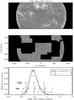 |
Fig. 1 Intensity data at 350μ from the James Clerk Maxwell telescope obtained by Lindsey et al. (1995). The upper figure shows, on a linear scale, part of the solar disk scanned by the JCMT on 1991 Feb. 9. The middle panel shows the same data without limb brightened regions and active regions, identified by eye. The lowest panel shows the distribution functions of relative intensities for both images (not counting zeros), and the locations of the model brightnesses at this wavelength (with model C set to unity), for both the F99 and VAL models. The intensities are linearly proportional to the temperature between 450 and 550 km above the visible continuum of the Sun. |
Now model “A” was originally built by VAL to match the 8th percentile in a distribution of Lyman continuum intensities observed with similar resolution by SKYLAB. The F99 models are updates including a large (230 K) upward shift in temperature of all models near the temperature minimum region (Maltby et al. 1986). Direct comparisons of the JCMT and SKYLAB intensity distributions are not possible, because the emergent intensity of the Lyman continuum is exponentially sensitive to the temperature, and is formed many scale heights higher in the chromosphere than 350μ radiation. Yet it is striking that model F99 A produces intensities below which only 1.8% of the pixels observed at 350μ are found. (The VAL model A produces intensities only at the 0.1% level).
We can get a sense in which a given point in the 350μ intensity distribution is going to be shifted in the intensity of the Lyman continuum, in the context of these models, as follows. Because temperatures at a given monochromatic optical depth in the F99 models increase monotonically from darkest (A) to brightest (F), at all temperatures within the chromospheres, the Lyman continuum will be brighter when the 350μ continuum is brighter. It is then clear that a given point in the distribution of infrared intensities will have its corresponding point at a much lower percentile in the UV continuum, owing to the exponential weighting of the Wien limit of the Planck function. Lastly, while the Lyman continuum is not formed in LTE, the systematic differences between the models which are of a very similar form imply that the source functions have at least the sense, if not the magnitude, of changes in the Planck function. Indeed Figs. 7 and 22 of VAL show, for example, that model E is 3 × brighter in the Lyman continuum than model B, but the 350μ continuum is just 1.14 × brighter.
We conclude that the model “A” temperatures of the upper photosphere are too low relative to model “C”, if model A is to represent more than a 1.8% of the number of occurrences in the 350μ intensity – hence temperature – distribution. A hint of this problem is present already in the VAL paper, where in their Fig. 22 brightness temperatures of the modeled intensities of A and B fell some 400 K below those then measured using sub-mm observations around 300 microns. Our analysis suggests that model B (or a model in between the A and B) could be a better choice for the minimum state of the least active Sun. The replacement of the model A by the model B would lead to approximately 2 times smaller forcing than reported by Shapiro and colleagues, as quoted by them.
3.3. The variable Sun in a stellar context
Taking the variations computed by S2011 at face value, we can place the Sun into the context of stars which have been observed photometrically for some decades. But this is not straightforward since no stars have been observed photometrically for centuries, and we must relate the TSI variations to the particular photometric indices that have been acquired in stars (Radick et al. 1998; Lockwood et al. 2007; Hall et al. 2009).
The long-term ( > 22 yr) variations computed by S2011, if present in solar-like stars, would appear only as secular changes in existing Sun-like stellar photometric records, because stellar data of the required precision are available only for the last 10 − 20 years. Therefore, unlike earlier work which has focussed on the statistical variances of stellar and solar fluxes, we adopt the following strategy to compare the solar and stellar data. First we compute annual b and y colors of the Sun from 1610 onwards, using the spectral irradiances computed by S2011 and the b, y filter profiles (they are centered at 470 and 550 nm respectively). Then we treat the 400 years of simulated solar data as an ensemble of stars each observed for 15 years, by dividing up the time series of b and y magnitudes into 53 individual “stellar” time series of 15 years duration, the first begining in 1610, the next 7.5 years later, etc. (This is an even, unbiased sampling). To this we add random noise with an amplitude of 0.12% which corresponds to the typical measurement errors associated with photometry using the Automated Photoelectric Telescopes, including the effects of slightly variable comparison stars. We also added in quadrature the 0.03% rms short term [< 22 yr] rotational/cyclic solar variability, but this is a small contributor. We then looked for secular changes in each of these 53 sun-observed as a star datasets by linear regression, yielding the fractional change in flux per year  , f = | δf | / ⟨ f ⟩ , as derived from a 15 year time series. This was repreated for 100 different random realizations of the noise. Histograms of were then plotted for comparison with stellar data whose individual values of were derived from the APT data. The peak of the solar data, without the added noise for comparison with stars, lies near = 5 × 10⁻⁵ yr-1. This is consistent with the irradiance changes of 1 W m-2 per decade noted between 1900 and 1950 in their reconstruction by S2011.
The stellar data come from 34 solar analogs (average spectral type G4V) observed by Automated Photometric Telescopes at Fairborn Observatory an average of 13 years (cf. Henry 1999) Their chromospheric emission ratios, as measured by the usual  , are within 0.15 dex of the solar value − 4.94. Stars included here are ones with non-zero net intrinsic variance after correction for comparison star variability (cf. Lockwood et al. 2007,Eq. on p. 290); about 30% of a larger sample fails this test.
The inclusion of a particular star in this histogram is influenced by the underlying comparison star variability, since all measurements are necessarily differential, one measures the brightness of the program star minus the mean of two comparison stars. The “cumulative probability of detection” plotted was determined from the distribution of comparison star variations in the sample, it varies from 25% at − 4.3 on the abscissa to 75% at − 4.0 on the abscissa. The stellar histogram is thus highly biased toward higher values of intrinsic variability and serves only to define a robust upper limit of expected solar variability.
Figure 2 shows that the reconstructed irradiance variations of S2011, as reflected in b + y photometry, lie tantalisingly close to, and below, those measured over the typical 15 year time span of existing measurements with APTs, in solar-like stars. The limiting factor in this plot is the variations in the brightness of the comparison stars used for comparative photometry. Thus, the variations computed by S2011 cannot be tested against current data.
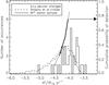 |
Fig. 2 A histogram of stellar secular behavior as measured by the fractional rate of change of b + y photometric flux with time, |

We should note that it is not so much the shape of this distribution that provides the critical test. The high-end tail of these distributions is a more critical parameter. For, just a few epochs of very large values in the irradiance reconstructions of S2011 are sufficient to make the large irradiance changes over centennial time scales. In this regard, we note that continued monitoring of stellar data in Fig. 2 is critical to answer if the solar behavior predicted by S2011 is anomalous. For, if the stellar data captured so far include some changes due to cycling activity, as expected, these stars will move to the left in time in the figure as the cycles make approach zero. If on the other hand, noise and secular changes are indeed dominating this distribution, the histogram will remain more or less the same shape. However, the locus of. probabilities of detection plotted in the figure may also move left approximately as t − 1/2 where t is the length of timeseries. Therefore, continued observations of stars will reveal if the computed Sun’s behavior is outside of the range of stellar behavior.
4. Conclusions
The results of S2011 are based upon a hypothesis – that the quiet solar radiance varies in time in proportion to the modulation potential, related to the global solar magnetic field – that currently is not directly testable by existing data. We have shown how the formulation adopted by S2011 means that regressions of irradiances from 1978 onwards with the modulation potential derived from neutron monitors, are different from the longer term assumed behavior (compare Eqs. (4) and (5)). This aspect of the work is shared by other reconstructions (e.g., Tapping et al. 2007; Krivova et al. 2010; Vieira et al. 2011). As formulated, S2011 reconstructed long term variations that are larger in part because of this difference. As S2011 specified, this algebra reflects the desire to use φ(t) as a long term proxy for solar activity under conditions like the Maunder Minimum, because since 1978 the minimum value of φ(t) is around 200 MV, whereas in earlier epochs it went effectively to zero.
The data presented here suggest that the reconstructed amplitudes of variation of the solar irradiance have been over-estimated by S2011. First, the amplitude of Shapiro et al.’s reconstructed variations is set by differences in the brightness of semi-empirical model photospheres “A” and “C” of F99. We have argued that the model “A” computed brightness is at the very minimum temperatures inferred from sub-mm data, formed in the temperature minimum region of the atmosphere. On the basis of the histograms of relative brightness, we suggest that the difference due to this factor alone should be closer to the difference in brightness between models “B” and “C”. In the Rayleigh-Jeans limit, the resulting amplitude is then reduced by a factor of about two, as reported in S2011. Second, there remains an unresolved debate concerning an observational link between magnetic fields on small and global scales (see Sects. 3.2.1 and 3.2.2). If the debate is resolved in favor of local control of small scale fields, then it will remain present in the absence of sunspots, and vary little on 22 yr and longer time scales (Judge & Saar 2007).
We have also demonstrated (Fig. 2) that the reconstructed solar time series appears to show secular changes within and below the ranges observed in b,y photometry of solar-like stars. However care is needed in interpreting this result, for at least two reasons. First, when looking for long-term ( > 22 yr, say) variations among the stars, there is no substitute for a time series of the duration needed. Thus, to see if the kinds of large secular changes reconstructed by S2011 over some 30 − 50 year periods (centered near the 1720, 1800, 1920 epochs) actually occur in stars, one must observe the stars for 30 − 50 years. Unfortunately we have data only for 15 years or so, and equally unfortunately, decadal time scales correspond to the typical variations associated with stellar spot cycles (Baliunas et al. 1995). A reasonable interpretation of our result is that we cannot yet discount such large secular solar variations on the basis of a comparison with stars, using the existing photometric data. It appears necessary to continue to observe this stellar sample for a couple more decades, to see if the histogram of, say  lies significantly to the left of that for , if, as might be expected, certain stars do not continue with their secular trends on this time scale. Second, we warn the reader that the spectral irradiance of the Sun as a star is not yet understood: the SIM measurements (Harder et al. 2009) suggest that b will vary little and that y will be out of phase with the irradiance. This is not compatible with
measured photometric behavior of the solar twin 18 Sco (Radick and Lockwood, papers presented at the 2011 SORCE meeting).
By “quiet Sun”, in this Note we refer to regions of the Sun seen away from active regions. It does not refer to a (fictional) atmosphere free of magnetic fields.
Acknowledgments
We thank G. de Toma and the referee for comments helping to clarify the text.
References
- Anderson, L., & Athay, R. 1989, ApJ, 346, 1010 [NASA ADS] [CrossRef] [Google Scholar]
- Baliunas, S. L., Donahue, R. A., Soon, W. H., et al. 1995, ApJ, 438, 269 [NASA ADS] [CrossRef] [Google Scholar]
- Cattaneo, F., & Hughes, D. W. 2001, Astron. Geophys., 42, 3.18 [Google Scholar]
- Eddy, J. A. 1976, Science, 192, 1189 [NASA ADS] [CrossRef] [PubMed] [Google Scholar]
- Feulner, G. 2011, Geophys. Res. Lett., 381, L16706 [NASA ADS] [CrossRef] [Google Scholar]
- Fontenla, J., White, O. R., Fox, P. A., Avrett, E. H., & Kurucz, R. L. 1999, ApJ, 518, 480 [NASA ADS] [CrossRef] [Google Scholar]
- Foukal, P. 2012, Sol. Phys., in press [Google Scholar]
- Foukal, P., & Milano, L. 2001, Geophys. Res. Lett., 28, 883 [NASA ADS] [CrossRef] [Google Scholar]
- Foukal, P., Bertello, L., Livingston, W. C., et al. 2009, Sol. Phys., 255, 229 [NASA ADS] [CrossRef] [Google Scholar]
- Gray, L. J., Beer, J., Geller, M., et al. 2010, Rev. Geophys., 48 [Google Scholar]
- Hagenaar, H. J. 2001, ApJ, 555, 448 [NASA ADS] [CrossRef] [Google Scholar]
- Hagenaar, H. J., Schrijver, C. J., & Title, A. M. 2003, ApJ, 584, 1107 [NASA ADS] [CrossRef] [Google Scholar]
- Hall, J. C., Henry, G. W., Lockwood, G. W., Skiff, B. A., & Saar, S. H. 2009, AJ, 138, 312 [NASA ADS] [CrossRef] [Google Scholar]
- Harder, J. W., Fontenla, J. M., Pilewskie, P., Richard, E. C., & Woods, T. N. 2009, Geophys. Res. Lett., 36, 7801 [NASA ADS] [CrossRef] [Google Scholar]
- Harvey, K. L. 1992, in Solar Electromagnetic Radiation Study for Solar Cycle, ed. R. F. Donnelly, 22, 113 [Google Scholar]
- Henry, G. W. 1999, PASP, 111, 845 [NASA ADS] [CrossRef] [Google Scholar]
- Judge, P. G., & Saar, S. H. 2007, ApJ, 663, 643 [NASA ADS] [CrossRef] [Google Scholar]
- Kleint, L., Berdyugina, S. V., Shapiro, A. I., & Bianda, M. 2010, A&A, 524, A37 [NASA ADS] [CrossRef] [EDP Sciences] [Google Scholar]
- Krivova, N. A., Vieira, L. E. A., & Solanki, S. K. 2010, J. Geophys. Res. (Space Physics), 115, 12112 [Google Scholar]
- Kuhn, J. R., & Libbrecht, K. G. 1991, ApJ, 381, L35 [NASA ADS] [CrossRef] [Google Scholar]
- Lindsey, C., Kopp, G., Clark, T. A., & Watt, G. 1995, ApJ, 453, 511 [NASA ADS] [CrossRef] [Google Scholar]
- Lites, B. W. 2011, ApJ, in press [Google Scholar]
- Livingston, W., White, O. R., Wallace, L., & Harvey, J. 2010, Mem. Soc. Astron. It., 81, 643 [NASA ADS] [Google Scholar]
- Lockwood, G. W., Skiff, B. A., Henry, G. W., et al. 2007, ApJSS, 171, 260 [NASA ADS] [CrossRef] [Google Scholar]
- Maltby, P., Avrett, E. H., Carlsson, M., Kjeldseth-Moe, O., & Kurucz, R. L. 1986, ApJ, 306, 284 [Google Scholar]
- Radick, R. R., Lockwood, G. W., Skiff, B. A., & Baliunas, S. L. 1998, ApJS, 118, 239 [NASA ADS] [CrossRef] [Google Scholar]
- Schmidt, G. A., Jungclaus, J. H., Ammann, C. M., et al. 2012, Geosci. Mod. Devel., 5, 185 [NASA ADS] [CrossRef] [Google Scholar]
- Shapiro, A. I., Schmutz, W., Rozanov, E., et al. 2011, A&A, 529, A67 [NASA ADS] [CrossRef] [EDP Sciences] [Google Scholar]
- Skumanich, A., Smythe, C., & Frazier, E. N. 1975, ApJ, 200, 747 [NASA ADS] [CrossRef] [Google Scholar]
- Steiner, O. 2010, in Magnetic Coupling between the Interior and Atmosphere of the Sun, eds. S. S. Hasan, & R. J. Rutten, 166 [Google Scholar]
- Steinhilber, F., Beer, J., & Fröhlich, C. 2009, Geophys. Res. Lett., 36, 19704 [Google Scholar]
- Stenflo, J. O. 2012, A&A, 541 [Google Scholar]
- Stenflo, J. O., & Kosovichev, A. G. 2012, ApJ, 745, 129 [NASA ADS] [CrossRef] [Google Scholar]
- Stott, P. A., Jones, G. S., & Mitchell, J. F. B. 2003, J. Climate, 16, 4079 [Google Scholar]
- Tapping, K. F., Boteler, D., Charbonneau, P., et al. 2007, Sol. Phys., 246, 309 [Google Scholar]
- Usoskin, I. G., Solanki, S. K., Schüssler, M., Mursula, K., & Alanko, K. 2003, Phys. Rev. Lett., 91(21), 211101 [Google Scholar]
- Usoskin, I. G., Alanko-Huotari, K., Kovaltsov, G. A., & Mursula, K. 2005, J. Geophys. Res. (Space Physics), 110, 12108 [Google Scholar]
- Vernazza, J., Avrett, E., & Loeser, R. 1981, ApJSS, 45, 635 [NASA ADS] [CrossRef] [Google Scholar]
- Vieira, L. E. A., Solanki, S. K., Krivova, N. A., & Usoskin, I. 2011, A&A, 531, A6 [NASA ADS] [CrossRef] [EDP Sciences] [Google Scholar]
- Wang, Y.-M., Lean, J. L., & Sheeley, Jr., N. R. 2005, ApJ, 625, 522 [Google Scholar]
All Figures
|
Fig. 1 Intensity data at 350μ from the James Clerk Maxwell telescope obtained by Lindsey et al. (1995). The upper figure shows, on a linear scale, part of the solar disk scanned by the JCMT on 1991 Feb. 9. The middle panel shows the same data without limb brightened regions and active regions, identified by eye. The lowest panel shows the distribution functions of relative intensities for both images (not counting zeros), and the locations of the model brightnesses at this wavelength (with model C set to unity), for both the F99 and VAL models. The intensities are linearly proportional to the temperature between 450 and 550 km above the visible continuum of the Sun. |
| In the text | |
|
Fig. 2 A histogram of stellar secular behavior as measured by the fractional rate of change of b + y photometric flux with time, |
| In the text | |
Current usage metrics show cumulative count of Article Views (full-text article views including HTML views, PDF and ePub downloads, according to the available data) and Abstracts Views on Vision4Press platform.
Data correspond to usage on the plateform after 2015. The current usage metrics is available 48-96 hours after online publication and is updated daily on week days.
Initial download of the metrics may take a while.