| Issue |
A&A
Volume 544, August 2012
|
|
|---|---|---|
| Article Number | A39 | |
| Number of page(s) | 10 | |
| Section | Interstellar and circumstellar matter | |
| DOI | https://doi.org/10.1051/0004-6361/201218861 | |
| Published online | 23 July 2012 | |
The infrared dust bubble N22: an expanding H ii region and the star formation around it
1 Xinjiang Astronomical Observatory, Chinese Academy of Sciences, 830011 Urumqi, PR China
e-mail: This email address is being protected from spambots. You need JavaScript enabled to view it.
2 Graduate University of the Chinese Academy of Sciences, 100080 Beijing, PR China
3 Key Laboratory of Radio Astronomy, Chinese Academy of Sciences, 830011 Urumqi, PR China
4 Department of Astronomy, Peking University, 100871 Beijing, PR China
Received: 21 January 2012
Accepted: 30 May 2012
Abstract
Aims. To increase the observational samples of star formation around expanding H ii regions, we analyzed the interstellar medium and star formation around N22.
Methods. We used data extracted from the seven large-scale surveys from infrared to radio wavelengths. In addition we used the JCMT⋆ observations of the J = 3−2 line of 12CO emission data released on CADC⋆⋆ and the 12CO J = 2−1 and J = 3−2 lines observed by the KOSMA⋆⋆⋆ 3 m telescope. We performed a multiwavelength study of bubble N22.
Results. A molecular shell composed of several clumps agrees very well with the border of N22, suggesting that its expansion is collecting the surrounding material. The high integrated 12CO line intensity ratio RICO(3 − 2)/ICO(2 − 1) (ranging from 0.7 to 1.14) implies that shocks have driven into the molecular clouds. We identify eleven possible O-type stars inside the H ii region, five of which are located in projection inside the cavity of the 20 cm radio continuum emission and are probably the exciting-star candidates of N22. Twenty-nine young stellar objects (YSOs) are distributed close to the dense cores of N22. We conclude that star formation is indeed active around N22; the formation of most of YSOs may have been triggered by the expanding of the H ii region. After comparing the dynamical age of N22 and the fragmentation time of the molecular shell, we suggest that radiation-driven compression of pre-existing dense clumps may be ongoing.
Key words: Hiiregions / ISM: clouds / stars: formation
James Clerk Maxwell Telescope, http://www.jach.hawaii.edu/JCMT/
The Canadian Astronomy Data Centre, http://www3.cadc-ccda.hia-iha.nrc-cnrc.gc.ca/
© ESO, 2012
1. Introduction
Using the Spitzer-GLIMPSE1 survey of the Galactic plane (Benjamin et al. 2003), Churchwell et al. (2006; 2007) cataloged almost 600 infrared (IR) dust bubbles. The IR dust bubbles are bordered by bright 8 μm shells (the photo-dissociation region (PDR)) that encloses bright 24 μm interiors. Of these IR dust bubbles, Deharveng et al. (2010) have studied a series of 102 ionized bubbles and concluded that 86% of these bubbles enclose H ii regions.
Deharveng et al. (2010) also concluded that star formation triggered by H ii regions may be an important process, especially for massive-star formation. Elmegreen (1998) and Deharveng et al. (2005) proposed various physical mechanisms of triggered the formation of stars around the H ii regions. Recently, one of the triggered processes called “collect and collapse”, proposed by Elmegreen & Lada (1977), has been studied in more detail inside the H ii region borders, and several observational studies supported that this mechanism is ongoing in several H ii regions (see e.g. Zavagno et al. 2007, 2010; Pomars et al. 2009; Petriella et al. 2010).
N22 is one of the northern IR dust bubbles cataloged by Churchwell et al. (2006). By checking the infrared (8 and 24 μm) image and the JCMT 12CO J = 3−2 data of N22, we found collected material, which indicates that triggered star formation may be taking place around N22. In this work, we present a molecular and IR study of the environment surrounding the IR dust bubble N22 to explore its surrounding ISM and search for signatures of star formation. We describe our data in Sect. 2, present N22 in Sect. 3, and the molecular analysis in Sect. 4 along with the exciting star(s) and star formation, Sect. 5 details our analysis of the star formation mechanism, and we summarize our findings in Sect. 6.
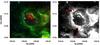 |
Fig. 1 Left: mid-IR emission of the IR dust bubble N22: Spitzer three-color image (4.5 μm = blue, 8 μm = green, and 24 μm = red). Right: the background shows the Spitzer-IRAC 8 μm emission. The two rectangles show the location of two IRDCs, which are named A and B. |
2. Data
Seven large-scale surveys were used in our study: 2MASS2, GLIMPSE, MIPSGAL3, NVSS4, GRS5, AKARI-BSC6, and the BGPS7 catalog.
The GLIMPSE and MIPSGAL (Carey et al. 2005) surveys were performed using the Spitzer Space Telescope (Werner et al. 2004). We used the mosaicked images from GLIMPSE and MIPSGAL acquired by Spitzer-IRAC (3.6, 4.5, 5.8 and 8 μm) (Fazio et al. 2004) and the MIPS instrument (24 and 70 μm) (Rieke et al. 2004), respectively. IRAC has an angular resolution of between 1 5 and 19. The MIPSGAL resolution at 24 μm is 6′′. The four far-infrared wavelengths of AKARI are centered at 65, 90, 140, and 160 μm, and their angular resolutions are 268, 268, 442 and 442, respectively (Murakami et al. 2007). The BGPS is a 1.1 mm continuum survey with an angular resolution of 33′′ (Aguirre et al. 2011). We also used the GLIMPSE Point-Source Catalog (GPSC), AKARI-BSC (Yamamura et al. 2010), and the BGPS catalog (Rosolowsky et al. 2010).
In addition, we used the 1.4 GHz radio continuum emission data extracted from the NVSS with an angular resolution of about 45′′ (Condon et al. 1998). For the molecular analysis, we used the James Clerk Maxwell Telescope (JCMT) observations of the J = 3−2 line of 12CO emission data released on CADC and the 13CO J = 1−0 from GRS performed by the Boston University and the Five College Radio Astronomy Observatory (FCRAO). The co-added spectral cubes of the JCMT 12CO J = 3−2 line were binned to 0.2 km s-1, and the data were smoothed with a 6′′ Gaussian kernel. The final spatial resolution of each cube is 16′′ (Smith et al. 2008), while the angular and spectral resolution of the GRS 13CO J = 1−0 are 46′′ and 0.2 km s-1 (Jackson et al. 2006).
We observed the 12CO J = 2−1 and J = 3−2 lines using the KOSMA 3 m telescope at Gornergrat, Switzerland in 2010 February. The half-power beamwidths of the telescope at observing frequencies of 230.538 GHz and 345.789 GHz are 130′′ and 80′′, and their corresponding system temperatures are about 233.5 and 357.8 K. The pointing and tracking accuracy is better than 10′′.
3. Presentation of N22
N22 is a complete IR dust bubble centered on  ,
,  ,
,  ) (Churchwell et al. 2006) with a radius of about 1.77 pc (Beaumont & Williams 2010). N22 was also known as an H ii region (G18.259−0.307) (Kolpak et al. 2003), its hydrogen recombination line velocity vLSR is ~50.9 km s-1. Kolpack and collaborators derived the near distance by comparison with the H i absorption data of G18.259−0.307, and obtained kinematic distances of ~ 4.1 ± 0.3 kpc. We adopt their vLSR and kinematic distance for N22.
Figure 1 (left) shows a Spitzer-IRAC and Spitzer-MIPSGAL three-color image of N22 (4.5 μm in blue, 8 μm in green, and 24 μm in red). The 24 μm emission corresponding to hot dust is distributed mainly toward the north of N22 (because of overexposure there are some bad data points in the peak of 24 μm). The PDR visible in the 8 μm emission is generally attributed to polycyclic aromatic hydrocarbon (PAH) molecules. Infrared emission from PAHs is a good tracer of ionization fronts (IF) because these large molecules are believed to be destroyed inside the ionized region, but are excited in the PDR by the radiation leaking from the H ii region (Pomars et al. 2009). The absorption in 8 μm usually indicates infrared dark clouds (IRDCs). Two absorptions appear in the gray map of 8 μm (right panel of Fig. 1), they were marked by two red rectangles. Because these two absorptions are bordered by bright 8 μm and the ionization fronts are distorted, we conclude that these two structures are indeed IRDCs (hereafter IRDC-A and IRDC-B). They have not been cataloged in the IRDC catalogs of Simon et al. (2006) and Peretto & Fuller (2009). However, IRDC-B has been identified by Watson et al. (2008) when they studied the nearby infrared dust bubble N21.
Figure 2 shows the Spitzer-IRAC emission at 4.5 μm (in blue), 8 μm (in green), and the NVSS radio continuum emission at 20 cm (in red and emphasized with white contours). The 20 cm emission, which is commonly attributed to the free-free emission from H ii regions, is bounded by 8 μm emission. The 20 cm emission shows a shell morphology, and a cavity can be clearly seen at its center. The strong 20 cm emission is distributed in the north of the shell, and shows an arc-like structure. Two peaks appears in the arc, and the stronger one is coincident with a small arc traced by 8 μm emission.
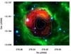 |
Fig. 2 Spitzer-IRAC emission at 4.5 μm (in blue), 8 μm (in green), and the NVSS radio continuum emission at 20 cm (in red and emphasized with white contours). The levels range from 0.05 to 0.15 by 0.02 Jy beam-1. The σrms of the NVSS data is 0.45 mJy beam-1. |
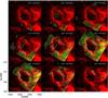 |
Fig. 3 Integrated velocity channel maps of the JCMT 12CO J = 3 − 2 emission every 1.5 km s-1 from 43.0 to 56.5 km s-1 (in green) superimposed on the 8 μm emission (in red). The contour levels of the 12CO J = 3 − 2 emission are 5, 10, 20, 35, and 55 K km s-1. The angular resolution of the JCMT 12CO J = 3 − 2 emission is 16′′. |
4. Molecular analysis and star formation
4.1. Molecular analysis
We used the 12CO J = 3−2 data cube from JCMT to analyze the molecular environment around N22. Figure 3 shows the integrated velocity channel maps of the 12CO J = 3−2 emission from 43.0 to 56.5 km s-1 in steps of 1.5 km s-1. Between 49.0 and 55.0 km s-1, several molecular clumps are distributed across the border of N22, which may indicate where the collect-and-collapse process could be taking place.
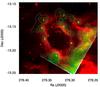 |
Fig. 4 JCMT 12CO J = 3−2 emission (in green) integrated between 40 and 60 km s-1. The contour levels of the 12CO J = 3−2 emission increase from 50.0 to 252.9 by 16.9 K km s-1. Red is the 8 μm emission. The yellow numbers are the ID of molecular cores. |
We integrated the JCMT 12CO J = 3−2 emission between 40 and 60 km s-1 (in green) over the 8 μm emission (in red) (see Fig. 4). Molecular cores 1−11 are clearly identifiable and are indeed distributed across the borders of N22, which as pointed out by Deharveng et al. (2005), may be indicative of the collect-and-collapse mechanism.
From Fig. 1 (right) and Fig. 4, we can see that the molecular cores 1 and 4 are associated with IRDC-A and IRDC-B. These two IRDCs distort the IF excited at the 8 μm, which are presently compressed by the ionized gas. They may have preexisted there before the H ii region expanded to reach them. This is consistent with the model “radiation-driven compression” (Deharveng et al. 2010). Based on the analysis above, we conclude that IRDC-B is physically associated with N22, and so is IRDC-A.
Assuming local thermodynamical equilibrium for the gas and an optically thick condition for the 12CO J = 3 − 2 line, we estimated the excitation temperature of the 12CO J = 3 − 2 line following the equation Tex = 16.6/ln [1 + 1/(Tmb/16.6 + 0.0024)] (Buckle et al. 2010), where Tmb is the main-beam temperature. Because it is difficult to obtain the optical depth τ from one transition of CO, we used the X factor between H2 and 12CO to estimate the column density of the 11 molecular cores. According to Shetty et al. (2011), the X factor is ~1−6 × 1020 cm-2 K-1 km-1 s. Here we assume X = 6 × 1020 cm-2 K-1 km-1 s and estimated the column density using the formula ![Mathematical equation: \begin{eqnarray*} N_{\rm H_{2}} = 6 \times 10^{20} W_{\rm CO}~\left[{\rm cm}^{-2}\right], \end{eqnarray*}](/articles/aa/full_html/2012/08/aa18861-12/aa18861-12-eq36.png) where WCO is the observed 12CO intensity, estimated following the equation
where WCO is the observed 12CO intensity, estimated following the equation 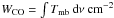 K km s-1. If the cloud cores are approximately spherical in shape, the mean H2 number density is nH2 = 1.62 × 10⁻¹⁹NH2/L, where L is the cloud core diameter in parsecs (pc). The mass is given by MH2 = 1.13 × 10⁻⁴μgm(H2)D2SNH2 [M⊙] (Buckle et al. 2010), where D is the distance in pc, S is the pixel area in arcsec2, μg = 1.36 is the mean atomic weight of the gas, and m(H2) is the mass of a hydrogen molecule. Finally, we list L, Tex, NH2, MH2, and nH2 of molecule cores 1 ~ 11 in Cols. 5−9 of Table 1, respectively. We used Gaussian fittings to obtain the peak temperature, velocity width, and central velocity. They are listed in Cols. 2−4 of Table 1.
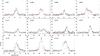 |
Fig. 5 JCMT 12CO J = 3−2 spectra at the peak of cores 1–11 are given in black, and GRS 13CO J = 1−0 spectra enlarged three times at the same region are delineated in red. |
The parameters of the molecular cores 1–11.
Figure 5 displays spectra at the peak of the molecule cores 1−11, the JCMT 12CO J = 3−2 spectra and GRS 13CO J = 1−0 spectra enlarged three times are depicted in black and red. The 12CO J = 3−2 spectra of #2, #4, #6, and #11 seem to show self-absorption, but corresponding 13CO J = 1−0 show no evidence of self-absorption. Taking into consider the integrated velocity channel maps (see Fig. 3), we suggest that 12CO J = 3−2 spectra of #2, #4, #6, and #11 include some different velocity components. Here we just consider the spectra main component associated to each clump of N22, which is centered at the velocity quoted in Table 1.
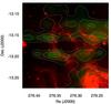 |
Fig. 6 Line intensity ratios RICO(3 − 2)/ICO(2 − 1) from KOSMA 12CO J = 3 − 2 and 12CO J = 2 − 1 is given in green, which is superimposed on the 8 μm emission in red. The contours range from 0.72 to 1.14 by 0.14. |
4.2. The expanding H ii region interacting with its surrounding material
As mentioned above, the morphology of N22 strongly suggests that the observed molecular shell has been swept and shaped by the expansion of N22 (see Fig. 4). The different transitions of 12CO can trace different molecular environments. To obtain the integrated intensity ratio of 12CO J = 3−2 to 12CO J = 2−1 (RICO(3−2)/ICO(2 − 1)), we convolved the 12CO J = 3−2 data to the same angular resolution as for 12CO J = 2−1. We performed an integrated 12CO line intensity ratio RICO(3−2)/ICO(2−1) for the whole bubble using the KOSMA data, which is between 0.7 and 1.14 (see Fig. 6). The ratios around N22 are higher than 0.8, which is much higher than previous measurements of individual Galactic Molecular Clouds (MCs) (0.55, Sanders et al. 1993) and even higher than the value (0.8) in the starburst galaxies M 82 (Guesten et al. 1993). The higher line ratios imply that shocks have driven into the MCs (Xu et al. 2011). Hereafter, the regions with higher line ratios (>0.8) are called “the active regions”. Our result indicates that the expanding H ii region is interacting with its surrounding material.
4.3. Exciting stars
No exciting stars of N22 have been described in the literature. However, according to the 20 cm flux and the estimated ionizing photon rate of N22, Beaumont & Williams (2010) stated that at least ten O9.5 stars are needed to produce the observed radio flux. To search for the exciting stars, we performed a photometric study of the infrared point sources inside the H ii region based on the GLIMPSE I Spring’07 and the 2MASS All-Sky Point Source Catalogs.
Taking into account that the exciting stars are expected to be in a PAHs hole, we just considered the sources inside the H ii region. They should be detected in the four Spitzer-IRAC bands and three 2MASS bands. Finally, we found 24 sources. Following the color criteria of Allen et al. (2004), we found 23 main-sequence (Class III) stars (see Fig. 7). Most of them are located inside the H ii region where the 20 cm radio continuum emission is weak.
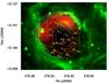 |
Fig. 7 Two color image, 8 μm in red and 20 cm in green with contours, which are similar to Fig. 2. The yellow plus show the location of the main sequence stars inside the H ii region. The red diamonds are the O-type stars. The white plus is the center of N22. |
To search for O-type stars, we used the J, H, and K apparent magnitudes obtained from the 2MASS Point Source Catalog to derive the absolute JHK magnitudes. We assumed a distance of 4.1 kpc and obtained the extinction for each source from the (J − H) vs. (H − K) color–color diagram. We also assumed the interstellar reddening law of Rieke & Lebofsky (1985) (AJ/AV = 0.282; AH/AV = 0.175 and AK/AV = 0.112) and the intrinsic colors (J − H)0 and (H − K)0 obtained from Martins & Plez (2006). By comparing the derived absolute JHK magnitudes with those tabulated by Martins & Plez (2006), we found 11 O-type stars inside the H ii region, these are #1, #4, #5, #7, #9, #10, #11, #13, #19, #21, and #22. Table 2 presents these sources with their 2MASS designation (Col. 2), apparent JHK magnitudes (Cols. 3 − 5), estimated extinctions (Col. 6), calculated absolute JHK magnitudes (Cols. 7 − 9), and indicates whether their derived spectral type coincides with an O-type in Col. 10.
Owing to the proper motion of ionizing star(s), they are not always located in the geometrical center of the H ii region. But because of the young ages of the IR dust bubble, the ionizing star(s) may be located near the geometrical center and still lie inside the cavity created by stellar wind. We can see that five O-type stars, #1, #4, #7, #10, and #13, are located in projection inside the cavity of the 20 cm radio continuum emission (see Fig. 7), they are probably the exciting stars of N22.
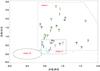 |
Fig. 8 GLIMPSE color–color diagram [5.8]-[8.0] versus [3.6]-[4.5] for sources within a circle of 4 |
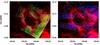 |
Fig. 9 Left: the background and contours are similar to Fig. 4. Right: the background and contours are similar to Fig. 6. The 32 sources of Spitzer-IRAC are symbolized with green diamonds. The blue stars are FIS-AKARI point sources, and triangles are BOLOCAM sources. The white plus is the center of N22. |
Exciting star candidates inside the H ii region.
4.4. SED fitting and star formation
Our analysis suggests that triggered star formation may take place around N22. To search for YSO candidates within a circle of 4 5 in radius centered at N22, we constructed a color–color diagram [5.8] − [8.0] versus [3.6] − [4.5] with the sources that have fluxes in the four Spitzer-IRAC bands. We used the photometric criteria of Allen et al. (2004) and the color criterion m4.5 − m8.0 > 1 (Robitaille et al. 2008) to identify class I and II YSOs (see Fig. 8). Finally, we selected 32 sources around N22 (see Fig. 9) and 10 of them, YSO-3, 4, 6, 9, 15, 19, 22, 24, 25, and 30, are cataloged by Robitaille et al. (2008) as Galactic midplane Spitzer red sources. Robitaille et al. (2008) pointed out that at most 0.4% of the intrinsically red sources selected by the color criterion m4.5 − m8.0 > 1 are galaxies and AGNs. Hence, there is a low probability of finding an extragalactic source in our small sample.
Near- and mid-IR fluxes of the 32 sources satisfying the photometric criteria of Allen et al. (2004) and the color criterion of m4.5 − m8.0 ≥ 1 around N22.
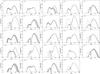 |
Fig. 10 SED of sources from which we obtained fluxes at 24 μm from the MIPS image. The sources are numbered according to Figs. 8 and 9. In each panel, the black line shows the best fit, and the gray lines show subsequent good fits. The dashed line shows the stellar photosphere corresponding to the central source of the best-fitting model, as it would look without circumstellar dust. The points are the input fluxes. |
The contributions from the disk and envelope of YSOs in the spectral energy distribution (SED) usually comes from long wavelengths, which are longer than ~10 microns and up to the millimeter region of the electromagnetic spectrum. Therefor longer wavelength data are needed to obtain a reliable SED for a YSO. We used the “phot” tool of Aladin (Bonnarel et al. 2000) to obtain the 24 μm fluxes of the sources from Spitzer-MIPS image. Using the conversion factor of 24 μm flux (7.17 Jy) toward its zero magnitude (Engelbracht et al. 2007), we calculated the 24 μm magnitudes. The SED-fitting tool developed by Robitaille et al. (2007) is available online8. We used this tool to fit the SED of all YSO candidates and selected the SED best-fit models according to the condition 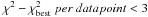 , where
  is the χ2 of the YSO best-fit model. Finally, we obtained the magnitudes of 24 sources and fitted their SED; the fitting results are listed in Table 3. Figure 10 shows the SED of these sources. Here we used the (J − H) vs. (H − K) color − color diagram from 2MASS to derive the visual extinction of those sources; the values are between 3 and 35 mag. Most of the values exceed 10 mag. According to Neckel & Klare (1980), the visual extinction toward star-forming regions generally exceeds 10 mag. Finally, we obtained the extinction between 10 and 35 mag.
The SED fitting allows us to obtain the physical parameters of the sources: the central source mass M ⋆ , the disk mass Mdisk, the envelope mass Menv, and the envelope accretion rate Ṁenv. According to these parameters, Robitaille et al. (2006) classified YSOs into three stages: stage 0/I objects have significant infalling envelopes and possibly disks, they have Ṁenv/M⋆ > 10-6 yr-1; stage II objects have optically thick disks (and possible remains of a tenuous infalling envelope), they have Mdisk/M⋆ > 10-6 and Ṁenv/M⋆ < 10-6 yr-1; and stage III objects have optically thin disks, they have Mdisk/M ⋆ < 10-6 and Ṁenv/M⋆ < 10-6 yr-1. From the SEDs of the sources (see Fig. 10), we found that YSO-3, 25 and 30 are stage II objects, YSO-4, 22 and 24 could be stage I and II objects, and we suggest that the remaining 18 sources are mainly stage I sources. We have to note that due to the absence of longer wavelengths data, the results of the stage I sources may have some uncertainty.
The fluxes for the six FIS-AKARI point sources.
We also found six FIS-AKARI point sources around N22, whose fluxes are listed in Cols. 3−6 of Table 4. Here, we used the Robitaille on-line tool to fit the FIS-AKARI point source fluxes by specifying “monochromatic” instead of “broad/narrow-band”. We did not fit source 2, because only two bands are detected. Finally, the SED fitting of the five FIS-AKARI sources indicates that they are all stage 0/I objects with masses ranging from 6.1 to 14.7 M⊙, their ages are about 103 ~ 105 yr (see Table 5). Figure 11 shows the SEDs of the five FIS-AKARI sources.
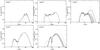 |
Fig. 11 SED of sources from the five FIS-AKARI sources around N22. The sources are numbered according to Table 5. |
Parameters derived from the SED fitting of five YSOs (FIS-AKARI point sources).
Most of the 24 sources and the five FIS-AKARI point sources lie close to the dense cores and the active region around the N22 (see Fig. 9). Thus star formation is indeed active around N22. The formation of these YSOs may have been triggered by the expanding H ii region.
From Fig. 9 (left), the five BOLOCAM sources can been seen across the borders of N22. Considering the gas-to-dust ratio of 100 (Enoch et al. 2006), we estimated the BOLOCAM source masses following the method of Rosolowsky et al. (2010): ![Mathematical equation: \begin{eqnarray*} M=\frac{13.1}{100} \left(\frac{D}{1~\rm kpc}\right)^2 \left(\frac{S_{\nu}}{1~\rm Jy}\right) \left[\frac{\rm exp(13.0~\rm K/{\it T})-1}{\rm exp(13.0/20)-1}\right]~[M_\odot], \end{eqnarray*}](/articles/aa/full_html/2012/08/aa18861-12/aa18861-12-eq115.png) where Sν is the total flux density of the BOLOCAM source in the catalog, dust temperature T = 20 K and distance D = 4.1 kpc. We obtained dust masses of the five BOLOCAM source (#1 to #5) of 7.1 M⊙, 0.8 M⊙, 18.7 M⊙, 7.7 M⊙, and 0.4 M⊙, respectively.
where Sν is the total flux density of the BOLOCAM source in the catalog, dust temperature T = 20 K and distance D = 4.1 kpc. We obtained dust masses of the five BOLOCAM source (#1 to #5) of 7.1 M⊙, 0.8 M⊙, 18.7 M⊙, 7.7 M⊙, and 0.4 M⊙, respectively.
5. Collect-and-collapse scenario?
We estimated the age of the H ii region and the fragmentation time to examine whether the “collect-and-collapse” mechanism is responsible for the star formation around the bubble N22.
To obtain the age of the H ii region, we used the model described by Dyson & Williams (1980) with a given radius R as ![Mathematical equation: \begin{eqnarray*} t(R)=\frac{4~R_{\rm s}}{7~c_{\rm s}}\left[\left(\frac{R}{R_{\rm s}}\right)^{7/4}-1\right], \end{eqnarray*}](/articles/aa/full_html/2012/08/aa18861-12/aa18861-12-eq120.png) where cs is the sound velocity in the ionized gas (cs = 10 km s-1) and Rs is the radius of the Strömgren sphere given by
where cs is the sound velocity in the ionized gas (cs = 10 km s-1) and Rs is the radius of the Strömgren sphere given by 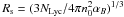 , where NLyc is the number of ionizing photons emitted by the star per second, n0 is the original ambient density, and αB = 2.6 × 10⁻¹³ cm3 s-1 is the hydrogen recombination coefficient to all levels above the ground level. Here we adopted a Lyman continuum photon flux of about 4.2 ~ 9.4 × 1049 ph s-1 (the total Lyman continuum photon flux of exciting stars, #1, #4, #7, #10, and #13, see Sect. 4.3), a radius of ~1.77 pc, and an original ambient density of ~1.0 × 103 cm-3. Finally, we derived a dynamical age of between 0.06 and 0.15 Myr for N22. To roughly estimate the original ambient density, we distributed the total mass of most dense cores, ~1.2 × 10⁴ M⊙ (exclude core 1 and core 4), over a sphere with a radius of 2 pc.
As mentioned above, several pieces of evidence indicate that the expansion of N22 collects the gas at its periphery. To determine whether the fragmentation could occur around N22, we estimated the fragmentation time of the collected layer according to the theoretical models of Whitworth et al. (1994b): ![Mathematical equation: \begin{eqnarray*} t_{\rm fragment}=1.56 \left(\frac{\alpha_{\rm s}}{0.2}\right)^{7/11} \left(\frac{N_{\rm Lyc}}{10^{49}}\right)^{-1/11} \left(\frac{n_0}{10^3}\right)^{-5/11}~[\rm Myr]. \end{eqnarray*}](/articles/aa/full_html/2012/08/aa18861-12/aa18861-12-eq131.png) Using a turbulent velocity αs ranging between 0.2 and 0.6 km s-1 (Whitworth et al. 1994b), we find that the fragmentation of the collected layer should occur between 1.36 and 2.93 Myr after its formation, which is later than the dynamical age. The fragmentation time is inferred by considering the uncertainty in the total Lyman continuum photon flux and turbulent velocity. Hence, the “collect-and-collapse” mechanism seems not to be responsible for the star formation activities around N22. Other processes such as the radiation-driven compression of pre-existing dense clumps (Deharveng et al. 2010) may operate here. From Figs. 1 (right) and 9 (left), we state that the compression of pre-existing dense clumps should be taking place mainly at the borders of IRDC-A and IRDC-B, which are interacting with N22. The YSOs (YSO-6, 7, 8, 9, 10, and AKARI-1) related to the IRDC-B are very likely formed by this process.
Using a turbulent velocity αs ranging between 0.2 and 0.6 km s-1 (Whitworth et al. 1994b), we find that the fragmentation of the collected layer should occur between 1.36 and 2.93 Myr after its formation, which is later than the dynamical age. The fragmentation time is inferred by considering the uncertainty in the total Lyman continuum photon flux and turbulent velocity. Hence, the “collect-and-collapse” mechanism seems not to be responsible for the star formation activities around N22. Other processes such as the radiation-driven compression of pre-existing dense clumps (Deharveng et al. 2010) may operate here. From Figs. 1 (right) and 9 (left), we state that the compression of pre-existing dense clumps should be taking place mainly at the borders of IRDC-A and IRDC-B, which are interacting with N22. The YSOs (YSO-6, 7, 8, 9, 10, and AKARI-1) related to the IRDC-B are very likely formed by this process.
6. Summary
Using multiwavelength surveys and archival data, we have studied the ISM around the bubble N22. The main results can be summarized as follows:
-
(1)
The PAH emission around N22 is detected at 8 μm and the radius is about 1.77 pc. The 24 μm emission reveals hot dust in the interior of the H ii region. The 20 cm emission is bounded by 8 μm emission and shows a shell morphology. The 20 cm emission is distributed mainly toward the north of the shell with two peaks. A cavity can be clearly seen at 20 cm emission, which may be created by the exciting-star(s) of N22.
-
(2)
A molecular shell composed of several clumps is distributed around the H ii region. Among the clumps, core 1 and core 4 are associated with IRDC-A and IRDC-B, which appear as dark extinction features against the Galactic background at mid-infrared wavelengths. The molecular shell has a total mass of about 21 000 M⊙.
-
(3)
The integrated KOSMA 12CO line intensity ratios RICO(3 − 2)/ICO(2 − 1) around N22 are measured at between 0.7 and 1.14. The higher line ratios (higher than 0.8) imply that shocks have driven into the MCs, this suggest that the expanding H ii region is interacting with the surrounding MCs.
-
(4)
We found 11 O-type star inside the H ii region, five of which are located in projection inside the cavity of the 20 cm radio continuum emission. We suggest that the five O-type stars may be a cluster exciting the bubble N22.
-
(5)
We discovered 24 YSOs that are very likely embedded in the molecular shell. Of these three YSOs are stage I-II objects, three YSOs are stage-II objects, and 18 YSOs are suggested to stage-I objects. Most of these 24 YSOs lie close to the dense cores and the active regions around the N22. We suggest that the formation of these YSOs are probably be triggered by the expanding H ii region.
-
(6)
We also fitted the SED of five FIS-AKARI point sources that are located close to the dense cores. They are all massive stars in stage 0/I.
-
(7)
By comparing the dynamical age of N22 and the fragmentation time of the molecular shell surrounding N22, we suggest that the triggered star formation mechanism “radiation-driven compression of pre-existing dense clumps” may work here. We state that IRDC-A and IRDC-B, which are the pre-existing dense clumps, are interacting with N22, and conclude that the YSOs related to the IRDC-B are very likely formed by this process.
James Clerk Maxwell Telescope, http://www.jach.hawaii.edu/JCMT/
The Canadian Astronomy Data Centre, http://www3.cadc-ccda.hia-iha.nrc-cnrc.gc.ca/
Galactic Legacy Infrared Mid-Plane Survey Extraordinaire http://irsa.ipac.caltech.edu/data/SPITZER/GLIMPSE/
Two Micron All Sky Survey, http://pegasus.phast.umass.edu/
NRAO VLA Sky Survey, http://www.cv.nrao.edu/nvss/
Galactic Ring Survey, http://www.bu.edu/galacticring/new_index.htm
Far-Infrared Survey (FIS) for AKARI Bright Source Catalog, http://heasarc.gsfc.nasa.gov/W3Browse/all/akaribsc.html
The Bolocam Galactic Plane Survey, http://milkyway.colorado.edu/bgps/
Acknowledgments
This work was funded by The National Natural Science Foundation of China under grant 10778703 and was partly supported by China Ministry of Science and Technology under State Key Development Program for Basic Research (2012CB821800) and The National Natural Science Foundation of China under grant 10873025.
References
- Aguirre, J., Ginsburg, A. G., Dunham, M. K., et al. 2011, ApJS, 192, 4 [NASA ADS] [CrossRef] [MathSciNet] [Google Scholar]
- Allen, L. E., Calvet, N., DAlessio, P., et al. 2004, ApJS, 154, 363 [NASA ADS] [CrossRef] [Google Scholar]
- Beaumont, C. N., & Williams, J. P. 2010, ApJ, 709, 791 [NASA ADS] [CrossRef] [Google Scholar]
- Benjamin, R. A., Churchwell, E., Babler, B. L., et al. 2003, PASP, 115, 953 [NASA ADS] [CrossRef] [Google Scholar]
- Bonnarel, F., Fernique, P., Bienayme, O., et al. 2000, A&AS, 143, 33 [NASA ADS] [CrossRef] [EDP Sciences] [Google Scholar]
- Buckle, J. V., Curtis, E. I., Roberts, J. F., et al. 2010, MNRAS, 401, 204 [NASA ADS] [CrossRef] [Google Scholar]
- Carey, S. J., Noriega-Crespo, A., Price, S. D., et al. 2005, BAAS, 37, 1252 [NASA ADS] [Google Scholar]
- Churchwell, E., Povich, M. S., Allen, D., et al. 2006, ApJ, 649, 759 [NASA ADS] [CrossRef] [Google Scholar]
- Churchwell, E., Watson, D. F., Povich, M. G., et al. 2007, ApJ, 670, 428 [NASA ADS] [CrossRef] [Google Scholar]
- Condon, J. J., Cotton, W. D., Greisen, E. W., et al. 1998, AJ, 115, 1693 [NASA ADS] [CrossRef] [Google Scholar]
- Deharveng, L., Zavagno, A., & Caplan, J. 2005, A&A, 433, 565 [NASA ADS] [CrossRef] [EDP Sciences] [Google Scholar]
- Deharveng, L., Schuller, F., Anderson, L. D., et al. 2010, A&A, 523, A6 [NASA ADS] [CrossRef] [EDP Sciences] [Google Scholar]
- Dyson, J. E., & Williams, D. A. 1980, Physics of the interstellar medium (New York: Halsted Press), 204 [Google Scholar]
- Elmegreen, B. G., & Lada, C. J. 1977, ApJ, 214, 725 [NASA ADS] [CrossRef] [Google Scholar]
- Elmegreen, B. G. 1998, in ASP Conf. Ser. 148, ed. C. E. Woodward, J. M. Schull, & H. A. Tronson, 150 [Google Scholar]
- Engelbracht, C. W., Blaylock, M., Su, K. Y. L., et al. 2007, PASP, 119, 994 [NASA ADS] [CrossRef] [Google Scholar]
- Enoch, M. L., Young, K. E., Glenn, J., et al. 2006, ApJ, 638, 293 [NASA ADS] [CrossRef] [Google Scholar]
- Fazio, G. G., Hora, J. L., Allen, L. E., et al. 2004, ApJS, 154, 10 [NASA ADS] [CrossRef] [Google Scholar]
- Guesten, R., Serabyn, E., Kasemann, C., et al. 1993, ApJ, 402, 537 [NASA ADS] [CrossRef] [Google Scholar]
- Jackson, J. M., Rathborne, J. M., Shah, R. Y., et al. 2006, ApJS, 163, 145 [NASA ADS] [CrossRef] [Google Scholar]
- Kolpak, M. A., Jackson, J. M., Bania, T. M., et al. 2003, ApJ, 582, 756 [NASA ADS] [CrossRef] [Google Scholar]
- Martins, F., & Plez, B. 2006, A&A, 457, 637 [NASA ADS] [CrossRef] [EDP Sciences] [Google Scholar]
- Martins, F., Schaerer, D., & Hillier, D. J. 2005, A&A, 436, 1049 [NASA ADS] [CrossRef] [EDP Sciences] [Google Scholar]
- Murakami, H., Baba, H., Barthel, P., et al. 2007, PASJ, 59, 369 [Google Scholar]
- Neckel, T., & Klare, G. 1980, A&AS, 42, 251 [NASA ADS] [Google Scholar]
- Peretto, N., & Fuller, G. A. 2009, A&A, 505, 405 [NASA ADS] [CrossRef] [EDP Sciences] [Google Scholar]
- Petriella, A., Paron, S., & Giacani, E. 2010, A&A, 513, A44 [NASA ADS] [CrossRef] [EDP Sciences] [Google Scholar]
- Pomarès, M., Zavagno, A., Deharveng, L., et al. 2009, A&A, 494, 987 [NASA ADS] [CrossRef] [EDP Sciences] [Google Scholar]
- Rieke, G. H., & Lebofsky, M. J. 1985, ApJ, 288, 618 [NASA ADS] [CrossRef] [Google Scholar]
- Rieke, G. H., Young, E. T., Engelbracht, C. W., et al. 2004, ApJS, 154, 25 [NASA ADS] [CrossRef] [Google Scholar]
- Robitaille, T. P., Whitney, B. A., Indebetouw, R., et al. 2006, ApJS, 167, 256 [NASA ADS] [CrossRef] [Google Scholar]
- Robitaille, T. P., Whitney, B. A., Indebetouw, R., et al. 2007, ApJS, 169, 328 [NASA ADS] [CrossRef] [Google Scholar]
- Robitaille, T. P., Meade, M. R., Babler, B. L., et al. 2008, AJ, 136, 2413 [NASA ADS] [CrossRef] [Google Scholar]
- Rosolowsky, E., Dunham, M. K., Ginsburg, A., et al. 2010, ApJS, 188, 123 [NASA ADS] [CrossRef] [Google Scholar]
- Sanders, D. B., Scoville, N. Z., Tilanus, R. P. J., Wang, Z., & Zhou, S. 1993, in Back to the Galaxy, eds. S. S. Holt, & F. Verter (Melville, NY: AIP), AIP Conf. Ser., 278, 311 [Google Scholar]
- Shetty, R., Glover, S. C., Dullemond, C. P., et al. 2011, MNRAS, 412, 1686 [NASA ADS] [CrossRef] [MathSciNet] [Google Scholar]
- Simon, R., Jackson, J. M., Rathborne, J. M., et al. 2006, ApJ, 639, 227 [NASA ADS] [CrossRef] [Google Scholar]
- Smith, H., Buckle, J., Hills, R., et al. 2008, Proc. SPIE, 7020, 70200Z1 [CrossRef] [Google Scholar]
- Watson, C., Povich, M. S., Churchwell, E. B., et al. 2008, ApJ, 681, 1341 [NASA ADS] [CrossRef] [Google Scholar]
- Werner, M. W., Roellig, T. L., Low, F. J., et al. 2004, ApJS, 154, 1 [Google Scholar]
- Whitworth, A. P., Bhattal, A. S., Chapman, M. J., et al. 1994, MNRAS, 268, 291 [NASA ADS] [CrossRef] [Google Scholar]
- Xu, J., Wang, J., & Miller, M. 2011, ApJ, 727, 81 [NASA ADS] [CrossRef] [Google Scholar]
- Yamamura, I., Makiuti, S., Ikeda, N., et al. 2010, VizieR Online Data Catalog, II/298 [Google Scholar]
- Zavagno, A., Pomars, M., Deharveng, L., et al. 2007, A&A, 472, 835 [NASA ADS] [CrossRef] [EDP Sciences] [Google Scholar]
- Zavagno, A., Anderson, L. D., Russeil, D., et al. 2010, A&A, 518, L101 [NASA ADS] [CrossRef] [EDP Sciences] [Google Scholar]
All Tables
Near- and mid-IR fluxes of the 32 sources satisfying the photometric criteria of Allen et al. (2004) and the color criterion of m4.5 − m8.0 ≥ 1 around N22.
All Figures
|
Fig. 1 Left: mid-IR emission of the IR dust bubble N22: Spitzer three-color image (4.5 μm = blue, 8 μm = green, and 24 μm = red). Right: the background shows the Spitzer-IRAC 8 μm emission. The two rectangles show the location of two IRDCs, which are named A and B. |
| In the text | |
|
Fig. 2 Spitzer-IRAC emission at 4.5 μm (in blue), 8 μm (in green), and the NVSS radio continuum emission at 20 cm (in red and emphasized with white contours). The levels range from 0.05 to 0.15 by 0.02 Jy beam-1. The σrms of the NVSS data is 0.45 mJy beam-1. |
| In the text | |
|
Fig. 3 Integrated velocity channel maps of the JCMT 12CO J = 3 − 2 emission every 1.5 km s-1 from 43.0 to 56.5 km s-1 (in green) superimposed on the 8 μm emission (in red). The contour levels of the 12CO J = 3 − 2 emission are 5, 10, 20, 35, and 55 K km s-1. The angular resolution of the JCMT 12CO J = 3 − 2 emission is 16′′. |
| In the text | |
|
Fig. 4 JCMT 12CO J = 3−2 emission (in green) integrated between 40 and 60 km s-1. The contour levels of the 12CO J = 3−2 emission increase from 50.0 to 252.9 by 16.9 K km s-1. Red is the 8 μm emission. The yellow numbers are the ID of molecular cores. |
| In the text | |
|
Fig. 5 JCMT 12CO J = 3−2 spectra at the peak of cores 1–11 are given in black, and GRS 13CO J = 1−0 spectra enlarged three times at the same region are delineated in red. |
| In the text | |
|
Fig. 6 Line intensity ratios RICO(3 − 2)/ICO(2 − 1) from KOSMA 12CO J = 3 − 2 and 12CO J = 2 − 1 is given in green, which is superimposed on the 8 μm emission in red. The contours range from 0.72 to 1.14 by 0.14. |
| In the text | |
|
Fig. 7 Two color image, 8 μm in red and 20 cm in green with contours, which are similar to Fig. 2. The yellow plus show the location of the main sequence stars inside the H ii region. The red diamonds are the O-type stars. The white plus is the center of N22. |
| In the text | |
|
Fig. 8 GLIMPSE color–color diagram [5.8]-[8.0] versus [3.6]-[4.5] for sources within a circle of 4 |
| In the text | |
|
Fig. 9 Left: the background and contours are similar to Fig. 4. Right: the background and contours are similar to Fig. 6. The 32 sources of Spitzer-IRAC are symbolized with green diamonds. The blue stars are FIS-AKARI point sources, and triangles are BOLOCAM sources. The white plus is the center of N22. |
| In the text | |
|
Fig. 10 SED of sources from which we obtained fluxes at 24 μm from the MIPS image. The sources are numbered according to Figs. 8 and 9. In each panel, the black line shows the best fit, and the gray lines show subsequent good fits. The dashed line shows the stellar photosphere corresponding to the central source of the best-fitting model, as it would look without circumstellar dust. The points are the input fluxes. |
| In the text | |
|
Fig. 11 SED of sources from the five FIS-AKARI sources around N22. The sources are numbered according to Table 5. |
| In the text | |
Current usage metrics show cumulative count of Article Views (full-text article views including HTML views, PDF and ePub downloads, according to the available data) and Abstracts Views on Vision4Press platform.
Data correspond to usage on the plateform after 2015. The current usage metrics is available 48-96 hours after online publication and is updated daily on week days.
Initial download of the metrics may take a while.