| Issue |
A&A
Volume 543, July 2012
|
|
|---|---|---|
| Article Number | A146 | |
| Number of page(s) | 16 | |
| Section | Stellar atmospheres | |
| DOI | https://doi.org/10.1051/0004-6361/201219167 | |
| Published online | 12 July 2012 | |
Magnetic activity and differential rotation in the young Sun-like stars KIC 7985370 and KIC 7765135⋆
1 Leibniz Institute for Astrophysics Potsdam (AIP), An der Sternwarte 16, 14482 Potsdam, Germany
e-mail: hefroehlich@aip.de
2 INAF, Osservatorio Astrofisico di Catania, via S. Sofia, 78, 95123 Catania, Italy
3 Università di Catania, Dipartimento di Fisica e Astronomia, via S. Sofia, 78, 95123 Catania, Italy
4 Astronomical Institute, Wrocław University, ul. Kopernika 11, 51-622 Wrocław, Poland
5 Departamento de Astrofísica y Ciencias de la Atmósfera, Universidad Complutense de Madrid, 28040 Madrid, Spain
Received: 5 March 2012
Accepted: 15 May 2012
Aims. We present a detailed study of the two Sun-like stars KIC 7985370 and KIC 7765135, to determine their activity level, spot distribution, and differential rotation. Both stars were previously discovered by us to be young stars and were observed by the NASA Kepler mission.
Methods. The fundamental stellar parameters (vsini, spectral type, Teff, log g, and [Fe/H]) were derived from optical spectroscopy by comparison with both standard-star and synthetic spectra. The spectra of the targets allowed us to study the chromospheric activity based on the emission in the core of hydrogen Hα and Ca ii infrared triplet (IRT) lines, which was revealed by the subtraction of inactive templates. The high-precision Kepler photometric data spanning over 229 days were then fitted with a robust spot model. Model selection and parameter estimation were performed in a Bayesian manner, using a Markov chain Monte Carlo method.
Results. We find that both stars are Sun-like (of G1.5 V spectral type) and have an age of about 100–200 Myr, based on their lithium content and kinematics. Their youth is confirmed by their high level of chromospheric activity, which is comparable to that displayed by the early G-type stars in the Pleiades cluster. The Balmer decrement and flux ratio of their Ca ii-IRT lines suggest that the formation of the core of these lines occurs mainly in optically thick regions that are analogous to solar plages. The spot model applied to the Kepler photometry requires at least seven persistent spots in the case of KIC 7985370 and nine spots in the case of KIC 7765135 to provide a satisfactory fit to the data. The assumption of the longevity of the star spots, whose area is allowed to evolve with time, is at the heart of our spot-modelling approach. On both stars, the surface differential rotation is Sun-like, with the high-latitude spots rotating slower than the low-latitude ones. We found, for both stars, a rather high value of the equator-to-pole differential rotation (dΩ ≈ 0.18 rad d-1), which disagrees with the predictions of some mean-field models of differential rotation for rapidly rotating stars. Our results agree instead with previous works on solar-type stars and other models that predict a higher latitudinal shear, increasing with equatorial angular velocity, that can vary during the magnetic cycle.
Key words: stars: activity / starspots / stars: rotation / stars: chromospheres / stars: individual: KIC 7985370 / stars: individual: KIC 7765135
Based on public Kepler data, on observations made with the Italian Telescopio Nazionale Galileo (TNG) operated by the Fundación Galileo Galilei – INAF at the Observatorio del Roque del los Muchachos, La Palma (Canary Islands), on observations collected at the 2.2-m telescope of the Centro Astronómico Hispano Alemán (CAHA) at Calar Alto (Almería, Spain), operated jointly by the Max-Planck-Institut für Astronomie and the Instituto de Astrofísica de Andalucía (CSIC), and on observations collected at the Catania Astrophysical Observatory (Italy).
© ESO, 2012
1. Introduction
In the Sun, magnetic activity is thought to be produced by a global-scale dynamo action arising from the coupling of convection and rotation (Parker 1955; Steenbeck et al. 1966). Young Sun-like stars rotate faster than the Sun and display a much higher level of magnetic activity in all atmospheric layers, which is likely due to a stronger dynamo action. They also display different types of activity from the Sun, such as larger and longer lasting spots in their photospheres, active longitude belts, the absence or different behaviour of their activity cycles, highly energetic flares, etc. These differences are likely related to the dynamo mechanism, which operates in rather different conditions in young stars mainly in terms of their rotation rate and internal structure. Understanding the properties of young suns and, particularly, their activity and rotation, is crucial to tracing the Sun and its environment back to their initial evolutionary stages.
The properties of the magnetoconvection in these stars seems to be strongly influenced by the Ω-effect that produces characteristic “wreaths” on large scales (Nelson et al. 2011). Although strong latitudinal variations in the differential rotation can be obtained by means of the combined role of thermal wind balance and geostrophy, the results of numerical simulations seem to depend strongly on the Reynolds number of the flow. This situation is at variance with the dynamo action in main sequence solar-type stars, where the role of the tachocline is instead essential in producing the α effect (Dikpati & Gilman 2001; Bonanno et al. 2002; Bonanno 2012).
It is still unclear whether a strong latitudinal differential rotation is common among rapidly rotating stars. Marsden et al. (2011) reported values of the absolute differential rotation dΩ in the range 0.08 − 0.45 rad d-1 for a sample of rapid rotators similar to and slightly more massive than the Sun. Despite the spread in values, it seems that dΩ is in any case larger than in the Sun. The measures of absolute differential rotation in a large sample of F- and early G-type stars based on the Fourier transform technique (Reiners & Schmitt 2003; Reiners 2006) show no indication of a decrease in this parameter with the rotation period, the highest values of dΩ instead being encountered for periods between two and three days. On the other hand, some calculations predict a moderate differential rotation, comparable to that of the Sun, for a Sun-like star rotating 20 times faster (e.g., Küker et al. 2011).
In addition, dΩ also seems to be a function of the stellar mass for main-sequence stars, increasing with their effective temperature, as shown, e.g., by Barnes et al. (2005). One of the largest values of differential rotation for a star noticeably cooler than the Sun was found by our research group (Frasca et al. 2011, hereafter Paper I) for KIC 8429280, a 50 Myr-old K2-type star, from the analysis of the light curve collected by the NASA Kepler spacecraft.
The highly precise photometry of Kepler (Borucki et al. 2010; Koch et al. 2010) coupled with a long and virtually uninterrupted coverage make these data unique for the study of the photospheric activity and differential rotation of late-type stars, as we demonstrated in our first work based on the analysis of Kepler data of spotted stars (Paper I).
However, whether star spots are indeed the most suited tracers of the surface rotation is still a matter of debate (for a different point of view, see Korhonen & Elstner 2011).
As for KIC 8429280 (Paper I), the two new targets KIC 7985370 (HD 189210 = 2MASS J19565974+4345083 = TYC 3149-1571-1) and KIC 7765135 (2MASS J19425057 +4324486 = TYC 3148-2163-1) were selected as active stars based on their optical variability and the cross-correlation of the ROSAT All-Sky Survey (RASS; Voges et al. 1999, 2000) with Tycho and Hipparcos catalogues (Perryman et al. 1997). With  and
and  , respectively, both stars are relatively bright ones in the Kepler field of view. Both of them were reported as variable by Pigulski et al. (2009), who searched for bright variable stars in the Kepler field of view with the ASAS3-North station. According to Uytterhoeven et al. (2011), the variability of KIC 7985370 could be due to a rotational modulation inferred from the first two quarters of Kepler data. The Kepler light curves readily show that these stars are rotationally variable with a period of about 2 − 3 days, which is typical of G-type stars in the Pleiades cluster (age ≈ 130 Myr, Barrado y Navascués et al. 2004). The estimates of their atmospheric parameters reported in the Kepler Input Catalog (KIC), which are based on Sloan photometry (for a revised temperature scale cf. Pinsonneault et al. 2012), suggested to us that these objects were similar to the Sun.
The analysis of the optical spectra collected by us confirmed that the stars are nearly identical to the Sun, but much younger and as such merit a detailed investigation. Applying the same techniques as in Paper I, we determined the basic stellar parameters (Sect. 3.1), the chromospheric activity (Sect. 3.2), and element abundances (Sect. 3.3). The kinematics of these stars is briefly discussed in Sect. 3.5. The Bayesian approach to spot modelling applied to the Kepler light curves is described in Sect. 4 and our results are presented and discussed in Sect. 5 with a particular focus on differential rotation.
2. Ground-based observations and data reduction
2.1. Spectroscopy
Two spectra of KIC 7985370 with a signal-to-noise ratio (S/N) of about 60 − 70 were collected at the M. G. Fracastoro station (Serra La Nave, Mt. Etna, 1750 m a.s.l.) of the Osservatorio Astrofisico di Catania (OAC, Italy) in July and October 2009. The 91-cm telescope of the OAC was equipped with FRESCO, a fiber-fed échelle spectrograph that, with the 300-lines/mm cross-disperser, covers the spectral range 4300 − 6800 Å with a resolution R = λ/Δλ ≈ 21 000.
Another spectrum of KIC 7985370 with S/N ≈ 120 was taken with SARG, the échelle spectrograph at the Italian Telescopio Nazionale Galileo (TNG, La Palma, Spain) on 2009 August 12 with the red grism and a slit width of 0 8. This spectrum, covering the 5500 − 11 000 Å wavelength range, has a resolution R ≈ 57 000.
The spectrum of KIC 7765135 was taken on 2009 October 3 with the Fiber Optics Cassegrain Échelle Spectrograph (FOCES; Pfeiffer et al. 1998) at the 2.2-m telescope of the Calar Alto Astronomical Observatory (CAHA, Almería, Spain). The 2048 × 2048 charged coupled device (CCD) detector Site#1d (pixel size = 24 μm) and the slit width of 400 μm give rise to a resolution R ≈ 28 000 and a S/N ≈ 100 in the red wavelength region with a 30-min exposure time.
Spectra of radial (RV) and rotational velocity (vsini) standard stars (Table 1), as well as bias, flat-field, and arc-lamp exposures were acquired during each observing run and used for the data reduction and analysis.
The data reduction was performed with the Echelle task of the IRAF1 package (see, e.g., Frasca et al. 2010; Catanzaro et al. 2010, for details).
Radial/rotational velocity standard stars.
2.2. Photometry
We used the focal-reducer CCD camera at the 91-cm telescope of OAC, on 2009 December 10, to perform standard photometry in the Johnson-Cousins B, V, RC, and IC bands. The data were reduced following standard steps of overscan region subtraction, master-bias subtraction, and division by average twilight flat-field images. The BVRCIC magnitudes were extracted from the corrected images by means of aperture photometry performed with DAOPHOT by using the IDL2 routine APER. Standard stars in the cluster NGC 7790 and the field of BL Lac (Stetson 2000) were used to calculate the zero points and the transformation coefficients to the Johnson-Cousins system. Photometric data derived in this work and JHKs magnitudes from 2MASS (Cutri et al. 2003) are summarized in Table 2.
Stellar parameters.
3. Target characterization from ground-based observations
3.1. Astrophysical parameters
The analysis of the high-resolution spectra was designed to measure the radial (RV) and projected rotational velocities (vsini), perform the MK spectral classification, and derive basic stellar parameters such as effective temperature (Teff), gravity (log g), and metallicity ([Fe/H]).
We computed the cross-correlation functions (CCFs) with the IRAF task fxcor by adopting spectra of late-F and G-type slowly rotating stars (Table 1), which had been acquired with the same setups and during the same observing nights as our targets. These stellar spectra were used for both the measure of RV and the determination of vsini by calibrating the full-width at half maximum (FWHM) of the CCF peak as a function of the vsini of their artificially broadened spectra (see, e.g., Guillout et al. 2009; Martínez-Arnáiz et al. 2010). We averaged the results from individual échelle orders as described, e.g., in Frasca et al. (2010) to get the final RV and vsini of our young Sun-like stars.
For KIC 7985370, we measured, within the errors, the same RV in the FRESCO spectra taken on 2009 July 10 (RV = −23.9 ± 0.4 km s-1) and 2009 October 4 (RV = −24.2 ± 0.4 km s-1), while a value of RV = −21.8 ± 0.2 km s-1 was derived from the SARG spectrum of 2009 August 12. This might be indicative of a true RV variation that is just above the 3-σ confidence level. However, much more spectra are needed to prove or disprove this RV variation and to ensure that the star is a single-lined spectroscopic binary.
For KIC 7765135, we only acquired one spectrum from which we derived an RV of −20.0 ± 0.2 km s-1.
Since we found no indication of binarity (visual or spectroscopic) in the literature for either star, we consider them as being single stars or, at most, single-lined spectroscopic binaries for which the putative companions are too faint to provide a significant contribution to either the optical spectrum or the Kepler photometry.
For the SARG spectrum, we used the ROTFIT code (Frasca et al. 2003, 2006) to evaluate Teff, log g, [Fe/H], and re-determine vsini, adopting a library of ELODIE Archive spectra of standard stars, as described in Paper I. To match the lower resolution (RFOCES = 28 000) of the FOCES spectrum, the ELODIE templates (RELODIE = 42 000) were convolved with a Gaussian kernel of  Å before running ROTFIT. We applied the ROTFIT code only to the échelle orders with a fairly good S/N, which span the ranges 5600 − 6700 Å and 4300 − 6800 Å for the SARG and FOCES spectra, respectively. The spectral regions heavily affected by telluric lines were excluded from the analysis. The adopted estimates for the stellar parameters and the associated uncertainties come from a weighted mean of the values derived for all the individual orders, as described in Paper I. We also applied this procedure to the FRESCO spectra of KIC 7985370, obtaining stellar parameters in very close agreement with those derived from the SARG spectrum.
ROTFIT also allowed us to measure vsini by fitting to the observed spectrum the spectra of slowly rotating standard stars artificially broadened at an increasing vsini and finding the minimum of χ2. For this purpose, we used the standard stars listed in Table 1 because their spectra were acquired with the same instrumental setup as that used for our targets, avoiding the introduction of any systematic error caused by a different resolution.
We obtained nearly the same values of the astrophysical parameters for both targets. They turn out to be very similar to the Sun, in terms of both spectral type and effective temperature, but considerably younger, as testified by the high lithium content in their photospheres (Sect. 3.3). Their average values and standard errors are reported in Table 2.
On the basis of these parameters and age estimates (Sects. 3.3 and 3.5), which are compatible with those of zero-age main-sequence (ZAMS) stars, we can roughly estimate their mass and radius as M = 1.15 ± 0.10 M⊙ and R = 1.1 ± 0.1 R⊙ from evolutionary tracks (e.g., Siess et al. 2000).
3.2. Chromospheric activity
The high level of magnetic activity in the chromosphere is displayed by the Ca ii IRT and Hα lines, which are strongly filled-in by emission (Figs. 1 and 2). The He i D3 (λ 5876 Å) absorption line is clearly visible in the spectra of our two young suns (Figs. 1 and 2). This is indicative of an upper chromosphere because a temperature of at least 10 000 K is required for its formation.
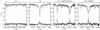 |
Fig. 1 Top of each panel: observed, continuum-normalized SARG spectrum of KIC 7985370 (solid line) in the He i D3, Hα, and Ca ii IRT regions together with the non-active stellar template (dotted red line). Bottom of each panel: difference between observed and template spectra. The residual Hα profile is plotted shifted downwards by 0.2 for the sake of clarity. The hatched areas represent the excess emission (absorption for He i) that have been integrated to get the net equivalent widths. |
We estimated the chromospheric emission level with the “spectral subtraction” technique (see, e.g., Frasca & Catalano 1994; Montes et al. 1995). This procedure is based on the subtraction of a reference “non-active” template compiled from observed spectra of slowly rotating stars of the same spectral type as the investigated active stars, but with a negligible level of chromospheric activity and an undetectable lithium line. The equivalent width of the lithium and helium absorption lines (WLi and WHe, respectively) and the net equivalent width (Wem) of the Ca ii IRT and Hα lines were measured from the spectrum obtained after subtracting the non-active template from the target and by then integrating the residual emission (absorption for the lithium and helium line) profile, which is represented by the hatched areas in Figs. 1 and 2.
We noted a significant variation in the Hα emission in the three spectra of KIC 7985370, with  ranging from 160 mÅ to 264 mÅ (Table 3).
The radiative losses in the chromospheric lines were evaluated by multiplying the average Wem by the continuum surface flux at the wavelength of the line, in the same way as in Frasca et al. (2010). The net equivalent widths and the chromospheric fluxes are reported in Table 3.
The Hβ net equivalent width could be measured only for KIC 7765135 because the SARG spectrum of KIC 7985370 does not include that wavelength region. In the FRESCO spectra, it is impossible to apply the subtraction technique, owing to the very low S/N in that spectral region, which prevented us from detecting such a tiny filling of the line.
For KIC 7765135, we measured a Balmer decrement FHα/FHβ = 4.3 ± 2.5 that is slightly larger than the values in the range 2 − 3 found by us for both KIC 8429280 (Paper I) and HD 171488 (Frasca et al. 2010). Accounting for the error, this ratio is however still compatible with optically thick emission by atmospheric features similar to solar and stellar plages (e.g., Buzasi 1989; Chester 1991) rather than to prominence-like structures, for which a Balmer decrement of the order of 10 is expected (e.g., Landman & Mongillo 1979; Hall & Ramsey 1992).
Line equivalent widths and chromospheric fluxes.
The Ca ii-IRT flux ratio, F8542/F8498 = 1.4 ± 0.9, is indicative of high optical depths and is in the range of the values found by Chester (1991) in solar plages. The optically thin emission from solar prominences gives rise instead to values of F8542/F8498 ~ 9. We measured a value of F8542/F8498 = 1.6 ± 1.0 for KIC 7985370, which is almost the same as that for KIC 7765135.
The chromospheric emission in both stars thus appears to originate mainly in surface regions similar to solar plages, while the quiet chromosphere and eventual prominences play a marginal role.
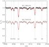 |
Fig. 3 Observed spectra (dots) of KIC 7985370 and KIC 7765135 (shifted downwards by 0.4) in the Li i λ 6707.8 Å region together with the synthetic spectra (full lines). |
Our adopted subtraction technique also allowed us to measure the lithium equivalent width cleaned of the contamination of the Fe i λ 6707.4 Å line, which is strongly blended with the nearby Li i line (Fig. 3). The lithium equivalent widths measured for KIC 7985370 (WLi = 155 ± 20 mÅ) and for KIC 7765135 (WLi = 160 ± 20 mÅ), which are immediately above the Pleiades upper envelope (Soderblom et al. 1993a), translates into a very high lithium abundance, log N(Li) = 3.0 ± 0.1, for both stars, based on the calibrations of Pavlenko & Magazzù (1996). The determination of the lithium abundance was refined in Sect. 3.3 by means of a spectral synthesis based on ATLAS9 atmospheric models (Kurucz 1993).
3.3. Abundance analysis
Since the spectral features of our two stars are relatively broad, it is difficult to find unblended lines for which equivalent widths can be reliably measured. To overcome this problem, the photospheric abundances were thus estimated by matching a rotationally broadened synthetic spectrum to the observed one. For this purpose, we divided each spectrum into 50 Å-wide segments, which were analysed separately. The spectral ranges 4450 − 8650 Å and 5600 − 7300 Å were used for the spectra of KIC 7765135 and KIC 7985370, respectively. The synthetic line profiles were computed with SYNTHE (Kurucz & Avrett 1981) using ATLAS9 (Kurucz 1993) atmospheric models. All models were calculated using the solar opacity distribution function and a microturbulence velocity ξ = 2 km s-1. For each segment, the abundance was determined by χ2 minimization. We used the spectral line list and atomic parameters from Castelli & Hubrig (2004), which is an update of the original list of Kurucz & Bell (1995).
The error in the abundance of one particular element was taken as the standard deviation of the mean of the abundances calculated for each segment. For elements whose lines occurred in only one or two segments, the error in the abundance was evaluated by varying the effective temperature and gravity within their uncertainties (as given in Table 2) and computing the abundance for Teff and log g values within these ranges. We found a variation of ≈0.1 dex in abundance due to temperature variation, but no significant variation when log g was varied. Thus, the uncertainty in temperature is probably the main source of error in the abundance estimation. In Fig. 3, we show an example of the matching between synthetic and observed spectra. To determine the Li abundance, we used the Li i λ6707 Å line, taking into account the hyperfine structure (Andersen et al. 1984). The abundances are given in Table 4.
Figure 4 compares the abundances derived for our targets and the solar values of Grevesse et al. (2010). With the exception of lithium, all other abundances are rather similar to those measured for the solar photosphere. In particular, we note that KIC 7765135 is ≈0.3 dex more metallic than the Sun, which confirms the results of ROTFIT (Table 2).
Abundances inferred for our two stars expressed in the form log N/Ntot.
As far as the lithium is concerned, we converted the abundance from log N/Ntot to log N/N(H) on a scale where log N(H) = 12, finding log N(Li) = 2.93 ± 0.10 and 2.87 ± 0.10 for KIC 7765135 and KIC 7985370, respectively. These values are smaller than, but marginally consistent with, those obtained from the equivalent widths and the calibrations of Pavlenko & Magazzù (1996) and reported in Sect. 3.2.
For early G-type stars, such as our targets, the lithium abundance does not provide a very strong constraint on their age. Their log N(Li) remains close to the initial lithium abundance for Population I stars (log N(Li) = 3.1−3.3) during their early life. It has been shown that stars with temperatures in the range Teff = 5900 ± 150 K display a significant lithium depletion (log N(Li) = 2.9) only after about 150 Myr (see, e.g., Sestito & Randich 2005). Thus, we can estimate an age of the order of 100−200 Myr for both stars with a lower limit of roughly 30−50 Myr, the lithium abundance being below the upper envelope of the α Per (age ≈ 50 Myr) and IC 2602 (age ≈ 30 Myr) clusters (Montes et al. 2001b; Sestito & Randich 2005). Moreover, the absence of a strong near-infrared (near-IR) excess in their spectral energy distributions (SEDs) (see Sect. 3.4) and of accretion signatures in the spectrum, allows us to exclude an age of a few million years for both stars that should already be in a post-T Tauri phase (age ≥ 10 − 20 Myr).
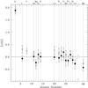 |
Fig. 4 Abundances found for KIC 7765135 (open circles) and for KIC 7985370 (filled circles) related to the solar ones. |
3.4. Spectral energy distributions
Our SEDs extending from the optical to the near-IR domain were obtained by merging our standard UBVRCIC photometry (Table 2) with JHKs magnitudes from the 2MASS catalogue (Cutri et al. 2003).
We used the grid of NextGen low-resolution synthetic spectra, with log g = 4.0 and 4.5 and solar metallicity by Hauschildt et al. (1999), to perform a fit to the SEDs. The effective temperature (Teff) was kept fixed to the value derived with ROTFIT (Table 2) for each target. The interstellar extinction (AV) was evaluated from the distance according to the rate of 0.8 mag/kpc found by Mikolajewska & Mikolajewski (1980) for the sky region around CI Cyg (very close to our targets). The Cardelli et al. (1989) extinction law with RV = 3.1 was used to evaluate the extinction in the other bands. Finally, the angular diameter (φ) that scales the synthetic surface flux over the stellar flux at Earth, was allowed to vary. The best-fit solution was found by minimizing the χ2 of the fit to the BVRCICJ data, which are dominated by the photospheric flux of the star and are not normally significantly affected by infrared (IR) excesses. The angular diameter derived for KIC 7985370, φ = 0.0895 mas, implies a distance d = 113 ± 15 pc, if we adopt a ZAMS radius of 1.1 R⊙ (Sect. 3.1). For KIC 7765135, we found φ = 0.0413 mas, which corresponds to d = 245 ± 30 pc, adopting again 1.1 R⊙. The error in the distance is estimated taking into account both a 0.1-R⊙ uncertainty in the stellar radius and the temperature error of about 100 K (see Table 2).
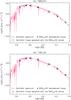 |
Fig. 5 Spectral energy distributions (dots) for KIC 7985370 (top panel) and KIC 7765135 (bottom panel). The NextGen synthetic spectrum at Teff = 5800 K scaled to the star distance is overplotted with continuous lines in each box. |
As apparent in Fig. 5, the SEDs are well-reproduced by the synthetic spectrum until the Ks band both for KIC 7985370 and KIC 7765135 and no excess is visible at near-IR wavelengths. This strengthens the spectroscopic determination of the effective temperature and ensures that these stars have certainly gone through the T Tauri phase, during which a thick and dense accretion disk gives rise to a conspicuous IR excess. The absence of mid- and far-IR data does not allow us to exclude the presence of thinner “debris” disks, similar to those found in a few Pleiades solar-type stars (Stauffer et al. 2005; Gorlova et al. 2006).
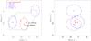 |
Fig. 6 (U, V) and (W, V) planes of our two young suns. We plotted the average position of each young stellar kinematic group with different symbols. The dotted line in the left panel demarcates the locus of the young-disk population (age < 2 Gyr) in the solar neighborhood, as defined by Eggen (1984, 1989). |
3.5. Kinematics
We used the radial velocities determined in Sect. 3.1 and the distances estimated in Sect. 3.4 together with measurements of proper motions taken from the Tycho-2 catalogue (Høg et al. 2000), to calculate Galactic space-velocity components (U, V, W), following the procedures described in Montes et al. (2001a). The values, listed in Table 2, are given in a right-handed coordinate system (which is positive towards the Galactic anti-centre, in the Galactic rotation direction, and towards the north Galactic pole, respectively). In the (U, V) and (W, V) Bottlinger diagrams (Fig. 6), we plotted the locus of our targets. Different symbols represent the central position given in the literature (see Montes et al. 2001a) of the five youngest and most well-documented moving groups (MGs) and superclusters (SCs): namely the Local Association (LA) or Pleiades MG (20 − 150 Myr), the IC 2391 SC (35 − 55 Myr), the Castor MG (200 Myr), the Ursa Major (UMa) MG or Sirius supercluster (300 Myr), and the Hyades SC (600 Myr).
The space velocities of these two Sun-like stars are consistent with those of the young-disk population (Fig. 6). On the basis of two different statistical methods (for further information, see Klutsch et al. 2010; Klutsch et al., in prep.), we determined their membership probability to each of the five aforementioned young stellar kinematic groups. Both KIC 7985370 and KIC 7765135 fall in the Local Association (LA) locus. With a probability of more than 70%, they turn out to be highly likely members of this moving group. Furthermore, such a result completely agrees with the age derived from the lithium abundance (Sect. 3.3).
4. Spot modelling of the Kepler light curves
4.1. Photometric data
All publicly available Kepler long-cadence time-series (Δt ≈ 30 min, Jenkins et al. 2010), spanning from 2009 May 2 to 2009 December 16, were analysed. These cover altogether 229 days and corresponds to the observing quarters 0 − 3 (Q0 − Q3), with the largest gap, about 4.5 days, appearing between Q1 and Q2.
To remove systematic trends in the Kepler light curves associated with the spacecraft, detector, and environment, and to prepare them for the analysis of star spots that we describe below, we used the software kepcotrend3. This procedure is based on cotrending basis vectors (CBV) that are calculated (and ranked) by means of singular value decomposition and describe the systematic trends present in the ensemble flux data for each CCD channel. We used the first two basis vectors for Q0 data, adopting between three and five CBV for the correction of longer data sets such as Q1, Q2, and Q3.
To check how the data rectification accomplished with kepcotrend is reflected in the outcome, the spot modelling has been done twice: with the rectified data (case A) as well as with the original data (case B).
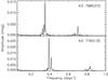 |
Fig. 7 Cleaned periodograms of the Kepler Q0+Q1+Q2+Q3 time series for KIC 7985370 (upper panel) and KIC 7765135 (lower panel). |
The power spectra of the Kepler time-series, cleaned by the spectral window according to Roberts et al. (1987), are displayed in Fig. 7. The lower panel of Fig. 7 clearly shows two main peaks for KIC 7765135, which are close in frequency (0.391 d-1 and 0.414 d-1). The corresponding periods are 2.560 ± 0.015 days and 2.407 ± 0.014 days, respectively. The period errors are inferred fromthe FWHM of the spectral window. The low-amplitude peaks at a frequency of ≈ 0.8 d-1 are overtones of the two main peaks. As visible from the upper panel of Fig. 7, the structure of the peaks for KIC 7985370 is more complex, with the maximum corresponding to 2.856 ± 0.019 days and a second peak, blended with the first one on its low frequency side, at 2.944 days. A third small peak corresponding to P = 3.090 days is also visible.
Such a double- or multiple-peaked periodogram is evidence of differential rotation. As Lanza et al. (1994) predicted, a photometric time series, if sufficiently accurate (ΔF/F = 10-5 − 10-6), may reveal a Sun-like latitudinal differential rotation.
An estimate of the inclination of the rotation axis with respect to the line of sight is very useful in constraining the spot model. When vsini, stellar radius R, and rotation period P are all known, the inclination of the rotation axis follows from 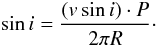 (1)In the absence of an accurate parallax value, the stellar radius cannot be derived from the effective temperature and luminosity. When we adopt the radius of a ZAMS star with the same effective temperature as our targets (Teff = 5800 K), R ≈ 1.1 R⊙, we get sini = 0.967 (i = 75° ± 15°) for both stars. However, as stated in Sect. 3.3, the lithium content cannot provide a firm lower limit to the ages of these stars, which might also be as young as a few 10 Myr (post-T Tauri phase). In the case of such a young age, a Teff = 5800 K would be reached by a star of 1.5 M⊙ at 10 Myr with a radius of about 2 R⊙ according to the evolutionary tracks by Siess et al. (2000), and an inclination of about 30° deduced.
4.2. Bayesian photometric imaging
Our imaging method is basically that of Paper I. However, as the duration of the light curves are now significantly longer, the introduction of additional free parameters is inevitable. The latitudinal dependence of the rotation frequency Ω(β) (Eq. (2)) now contains a sin4β-term and, more importantly, the prescription for spot area evolution is much more detailed. Furthermore, the likelihood function (Eq. (3)) is generalized by taking into account an unknown linear trend in the data. To tackle the problem of strong correlations between some parameters, an essential new ingredient is the usage of an orthogonalized parameter space, where the steered random walk of the Markov chains is performed. For the sake of clarity and owing to these new features, the basics of the method are explained in this section, although they can also be found in Paper I. A full account of the method is deferred to a forthcoming Paper (Fröhlich, in prep.).
A light-curve fitting that represents spots as dark and circular regions has the advantage of reducing the dimensionality of the problem and promptly provides us with average parameters (area, flux contrast, position, etc.) for each photospheric active region. There are, of course, other techniques, which are based on different assumptions, to reconstruct surface features photometrically as the inversion of Kepler light curves (cf., e.g. Brown et al. 2011).
Our aim is to present a low-dimensional spot model, with only a few spots that fits reasonably well the data regardless of very low-amplitude details that require a high degree of complexity. In a Bayesian context, this claim could be even quantified. One should ideally estimate the so-called evidence, namely the integral over the posterior probability distribution. This provides a measure of the probability of a n-spot model and, therefore, allows one to constrain the number of spots n that are really needed. For numerical reasons, we are compelled to resort instead to the less demanding Bayesian information criterion (BIC) of Schwarz (1978). This or any other related criterion expresses Occam’s razor in mathematical terms without the need to compute numerically the integral over the posterior probability distribution. Unfortunately, we have to admit that – owing to the unprecedentedly high accuracy of the Kepler data – we could not constrain n by applying the BIC. There is obviously more information in the data than our most elaborate model is able to account for.
Dorren’s (1987) analytical star-spot model, generalized to a quadratic limb-darkening law, was used. The two coefficients were taken from the tables of Claret & Bloemen (2011) for a microturbulence velocity of ξ = 2 km s-1 and used for both the unperturbed photosphere and the spots.
Four parameters describe the star as a whole: one is the cosine of the inclination angle i. Three parameters (A,B, and C) describe the latitudinal dependence of the angular velocity. With β being the latitude value, the angular velocity Ω is parameterized by a series expansion using Legendre polynomials  (2)The equatorial angular velocity is Ωeq = A − 3B/2 + 15C/8 and the equator-to-pole differential rotation dΩ = 15B/2 + 105C/8. In the case of the equator rotating faster than the poles, dΩ is negative. In what follows, the minus sign is suppressed, and only the absolute value | dΩ | is given. Both stars are definitely rotating like the Sun.
As in Paper I, all star spots have the same intensity κ relative to the unspotted photosphere and are characterized by two position coordinates (latitude and initial longitude) and by their radius. All these are free parameters in the model. Other spot parameters are the rotation period, which defines the spot longitude at any time and is tied to the latitude via Eq. (2). The hemisphere, to which a spot belongs to, is to be found by trial and error. Further parameters describe the spot area evolution.
As our photometric analysis is designed mainly to estimate the level of surface differential rotation, our focus is on long-lived spots, i.e. longevity of star spots is at the heart of our approach. To obtain, in view of the extraordinary length of the time series, a satisfying fit, more flexibility has been given to spot area evolution with respect to Paper I. It is now parameterized by up to eight parameters.
 |
Fig. 8 Kepler light curve with best fit (solid red line, second case-A solution of Table 5) overplotted. The residuals, shown at the top, are ± 2.14 mmag and obviously inhomogeneous from one part of the light curve to another. |
The spot area is given in units of the star’s cross-section. Area evolution is assumed to proceed basically linearly with time. The underlying physical reason for this is that, at least in the case of a decaying spot, the slope of the area-time relation is somehow related to the turbulent magnetic diffusivity. With the aim of enhancing flexibility and to describe the waxing and waning of a spot, three consecutive slope values are considered. The time derivative of the spot area is then a mere step function over time, and the step height measures the increase/decrease in area per day. Hence, there are six free parameters: three slope values, two dates of slope change, and the logarithm of spot area at some point of the time series. An additional feature is that to prevent sharp bends in the spot area evolution, some smoothing is introduced. Each date where the slope changes is replaced by a time interval to which we assign a slope that is the linear interpolation of the two adjacent values. This ensures that the second order time derivative of spot area is a mere step function of time, described by six parameters. To get the integrated area itself as function of time, two constants of integration enter, thus bringing the number of free parameters to describe a spot’s area evolution to a total of eight.
In addition to the free parameters of the model, there are the ones derived. An example is the rotational period, which follows from the longitudes of the spot centre at the beginning of the time series and at its end.
All parameters are estimated in a Bayesian manner, i.e. their mean values as well as the corresponding uncertainties follow straightforwardly from the data alone. To maintain a flat prior distribution in parameter space, all dimensional parameters such as the periods or spot radii must actually be described by their logarithms. Only then will the posterior probability distribution for a period be consistent with that of a frequency and likewise the posterior for a radius with that of an area, i.e. it does not matter whether one considers periods instead of frequencies or radii instead of areas.
The likelihood function (Eq. (3)) assumes that the measurement errors have a Gaussian distribution in the magnitude domain. This is justified as long as the S/N does not vary with changing magnitude, as in the case of our data that span a full variation range smaller than 0.1 mag. This has the invaluable advantage that the likelihood function can be analytically integrated over the measurement error σ, offset c0, and linear trend d0. To perform the integration over σ, one has to use Jeffreys’ 1/σ-prior (cf. Kass & Wassermann 1996). The resulting mean likelihood depends on only the spot-modelling parameters p1...pM. This takes into account all possible error values, offsets, and linear trends. By multiplying this with the prior, which is assumed to be constant in parameter space, one gets the posterior density distribution. All interesting quantities, like parameter averages and confidence intervals, are then obtained by marginalization.
With the N magnitude values di measured at times ti, their standard deviations σi, the model magnitudes f0(ti,p1...pM), offset c0, and trend d0, the likelihood function is given by  (3)We set σi = si·σ, with relative errors si being normalized according to
  .
.
By sampling the parameter space, we estimated the parameters using the Markov chain Monte Carlo (MCMC) method (cf. Press et al. 2007).
Often parameter values are highly correlated. As MCMC performs best in an orthogonalized parameter space, we converted all parameters using a principal component analysis based on singular value decomposition (cf. Press et al. 2007). Each parameter in this abstract space is linearly dependent on all of the original parameters. The reconstruction of the original parameter values can be done by exploiting a subspace of this orthogonalized parameter space. The dimension of this subspace, i.e. the number of degrees of freedom, is then found to be lower by roughly one third or even more than the number of original parameters.
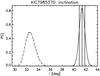 |
Fig. 9 Determination of the stellar inclination from Kepler photometry. Mean and 68-per-cent confidence interval are indicated by vertical lines (case A only). Dashed: the corresponding marginal distribution for the original data with linear trends removed (case B). |
Three seven-spot solutions for KIC 7985370.
4.3. Results
4.3.1. KIC 7985370
We identified 11 gaps longer than an hour and 2 additional small jumps in the light curve (Fig. 8). The data set was accordingly divided into 14 parts. Each part was assigned its individual error level, offset, and, in case B (i.e. non-rectified data), linear trend. Hence, the likelihood (Eq. (3)) is the product of 14 independent contributions.
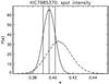 |
Fig. 10 Spot intensity related tothe unspotted photosphere. Mean and 68-per-cent confidence interval are indicated by vertical lines (case A only). Dashed: the corresponding marginal distribution for the original data with linear trends removed (case B). |
KIC 7985370’s inclination value i was – to be honest – ill-defined by the spot model applied to the Kepler photometry. With only six spots, the MCMC indeed identified very dark spots (κ ≈ 0) at very low inclination (i ≈ 10°). However, even for these unrealistic solutions the equator-to-pole differential rotations was 0.18 rad d-1. Only with seven spots and allowing for sufficient amount of spot evolution did we arrive at acceptable inclination values (Fig. 9) and spot intensities (Fig. 10). When the inclination is fixed to the spectroscopically derived value of i = 75°, the residuals are rather high, ± 2.46 mmag, exceeding the residuals of our best-fit solution ( ± 2.14 mmag) by far. Nevertheless, the details of the solution with fixed inclination are also included in Table 5, where the results are presented.
Improving the seven-spot solution by adding an eighth spot formally leads to a tighter fit. As the new spot proves to be ephemeral, lasting only six rotations, it neither constrains the differential rotation nor adds any significant insight (one can always get a better result by adding short-lived features).
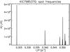 |
Fig. 11 All seven marginal distributions (case A) of the spot frequencies. The three frequencies (0.324, 0.340, and 0.350 d-1) seen in the low-resolution Fourier spectrum (Fig. 7) are confirmed by the results of our spot model. |
The marginal distributions of all spot frequencies (case A only), combined into one plot, are shown in Fig. 11.
From the three parameters describing the star’s surface rotation, A,B, and C, the equatorial rotational period (Fig. 12) and the equator-to-pole differential rotation (Fig. 13) follow. The latter amounts to  rad d-1 (case A) and 0.1729 ± 0.0002 rad d-1 (case B), respectively. The difference is significant, considering the formal errors, albeit very small. In the case of fixed inclination (i = 75°), the differential rotation would be slightly enhanced, 0.1839 ± 0.0002 rad d-1.
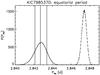 |
Fig. 12 Equatorial period of the star. Mean and 68-per-cent confidence interval are indicated by vertical lines (case A only). Dashed: the corresponding marginal distribution for the original data with linear trends removed (case B). |
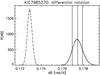 |
Fig. 13 Equator-to-pole differential rotation of the star. Mean and 68-per-cent confidence interval are indicated by vertical lines (case A only). Dashed: the corresponding marginal distribution for the original data with linear trends removed (case B). |
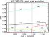 |
Fig. 14 Spot area evolution (case A). Area is in units of the star’s cross-section. Vertical lines mark the boundaries of the Q0 to Q3 quarters of data. A number in parenthesis indicates the spot number. |
The spot area evolution is depicted in Fig. 14. The sudden appearance of spot # 7 seems to be an artefact. It falls into the gap between the end of the Q2 data and the beginning of the Q3 data. On the other hand, the sudden disappearance of spot # 3 is unrelated to any switching from one part of the light curve to the next one. The fall in area of spot # 1 at the end of the time series is somehow mirrored by an increase in the size of spot # 5. However, this highlights a flaw due to too much freedom in describing the spot area evolution.
Expectation values with 1-σ confidence limits for various parameters are also quoted in Table 5.
One should be aware that there is more than one solution for each case. The second case-A solution presented in Table 5 is the one that has the lowest residuals found so far. There is an other well-relaxed seven-spot solution with slightly larger residuals nearby in parameter space. In that solution, the fastest spot (# 2), which comes into existence near the end of the time series at JD ~ 2 455 135, is located at a more southern latitude of − 21°, resulting in a slightly higher differential rotation. All other spots are virtually unaffected. Further details of this second solution are given in Table 6.
4.3.2. KIC 7765135
We identified 11 gaps longer than an hour and 3 additional small jumps in the light curve (Fig. 15). The data set was accordingly divided into 15 parts. Each part was assigned its individual error level, offset, and, in case B (i.e. non-rectified data), linear trend. Hence, the likelihood function (Eq. (3)) is the product of 15 independent contributions.
As the inclination is photometrically ill-defined, we fixed it to the spectroscopically derived value of i = 75°.
Despite the addition of two spots, the residuals, ± 2.35 mmag, exceed those of the seven-spot model of KIC 7985370 ( ± 2.14 mmag). This is not due to the fainter magnitude of KIC 7765135 than to KIC 7985370, because the photometric uncertainties are typically 0.047 mmag for the former and 0.022 mmag for the latter. The reason may instead be that three of the nine spots are definitely short-lived with a life span as short as two months (cf. Fig. 20), which is less than twice the lapping time of 38 days between the fastest and the slowest spot. We have to admit that dealing with nine spots almost exceeds the capabilities the MCMC technique since the method’s relaxation time then becomes prohibitively long.
A second pair of seven-spot solutions for KIC 7985370.
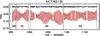 |
Fig. 15 Kepler light curve with best fit (solid red line, case-A solution of Table 7) overplotted. The residuals, shown at the top, are ± 2.35 mmag and obviously inhomogeneous from one part of the light curve to another, hence, the stated ± 2.35 mmag is to be considered an overall average. |
The marginal distribution of the spot rest intensity is shown in Fig. 16.
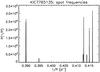 |
Fig. 17 Marginal distributions of the frequency for all the nine spots. The frequency values group around the two principal frequencies (0.391 and 0.414 d-1) seen already in the Fourier spectrum (Fig. 7), which is the reason for the obvious “beating” phenomenon in Fig. 15 with a period of 40 days. The shortest and the longest frequency are a superposition of two frequencies. |
The marginal distributions of the nine spot frequencies (case A only), combined into one plot, are shown in Fig. 17.
From the three parameters describing the star’s surface rotation, A,B, and C, the equatorial rotational period (Fig. 18) and the equator-to-pole differential rotation (Fig. 19) follows. The latter amounts to 0.1760 ± 0.0003 rad d-1 (case A) and  rad d-1 (case B), respectively. As for KIC 7985370, the difference is small, but nevertheless significant.
The level of differential rotation does not depend on the number of spots considered. Neglecting the three short-lived spots, i.e. considering a six-spot model, would result in an equator-to-pole shear of 0.1777 ± 0.0006 rad d-1.
The inclination does not significantly affect dΩ. Decreasing the inclination from the adopted value of i = 75° to 45° would indeed result in a marginally higher differential rotation by three to four per cent. This is quite understandable: inclination affects latitudes, but hardly periods.
A cursory glance cast at the beating pattern (Fig. 15) reveals a lapping time Pbeat ~ 40 days, which is nearly exactly the lapping time of 40.3 days from the two peaks of the cleaned periodogram (Fig. 7). From these 40.3 days, one is already able to estimate the minimum value of the differential rotation as 2π/Pbeat ~ 0.156 rad d-1, which is not far from that derived by the model.
The spot area evolution (case A) is depicted in Fig. 20. The overwhelmingly large southern spot – at the beginning it fills a large extent of the southern hemisphere – may be an artefact. Owing to its southern location, its contribution to the light curve is rather modest. Perhaps it is actually a feature in the northern hemisphere, a non-circular extension of spot # 2. To prevent spot overlap, spot # 8 had to be moved to the southern hemisphere. The reader should be aware that even in the case of a large spot, the whole spot region has been assigned the angular velocity of its centre. Differential rotation is, to be exact, incompatible with a fixed circular shape. This is a shortcoming of our simple model.
In the case of KIC 7765135, we cannot exclude that spot area evolution is partly driven by the need to avoid the overlapping of spots.
Expectation values with 1-σ confidence limits for various parameters are compiled in Table 7.
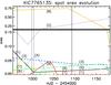 |
Fig. 20 Same as Fig. 14, for KIC 7765135. Three of the nine spots (# 4, # 7, and # 9) are short-lived ones. Note the change in scale in the upper part! |
Two nine-spot solutions for KIC 7765135 with inclination being fixed to i = 75°.
5. Discussion
5.1. Chromospheric and coronal activity
To compare with the chromospheric activity of stars similar to our targets, we considered 18 stars in the Pleiades cluster among those investigated by Soderblom et al. (1993b), that have an early-G spectral type or an effective temperature close to those of our targets and a vsini between 4 km s-1 and 18 km s-1. With a spectral subtraction analysis, they found values of the net Hα emission between 100 mÅ and 500 mÅ and surface fluxes ranging from 1.0 × 10⁶ to 2.9 × 10⁶ erg cm-2 s-1. The net emission filling the core of the Ca ii-λ8542 line ranges from about 300 mÅ to 600 mÅ and the corresponding flux is in the range 1.0−2.7 × 10⁶ erg cm-2 s-1. The values of these activity indicators for our two targets are within all of these ranges, suggesting an activity level comparable to the Pleiades stars (age ~ 130 Myr). The X-ray luminosity of these Pleiades members, as evaluated by Stauffer et al. (1994) and Marino et al. (2003), is in the range log LX = 28.7 − 29.7, which is just below the saturation threshold of log LX = 30.0 found by Pizzolato et al. (2003) for Sun-like stars. Moreover, according to the works of Pizzolato et al. (2003) and Soderblom et al. (1993b), the saturation would occur for rotation periods shorter than about 2.0 days. Another helpful study of the chromospheric activity in stars belonging to the young open clusters IC 2391 and IC 2602 (age ≈ 30−50 Myr) shows that the chromospheric flux measured in the core of Ca ii − λ8542 line saturates at a value of  (Marsden et al. 2009). A similar behaviour was previously found for the Pleiades by Soderblom et al. (1993b). The
  values of − 4.5 and − 4.6 that can be derived for KIC 7985370 and KIC 7765135, respectively, are lower than, but not very far from, this saturation level. From the ROSAT X-ray count and the distance quoted in Table 2, we evaluated the X-ray luminosity of KIC 7985370 using the relation proposed by Fleming et al. (1995), LX = 4πd2(8.31 + 5.30 HR1) × 10-12 erg s-1, where the hardness ratio is HR1 = 0.23 (Voges et al. 2000). The value of
 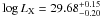 confirms the non-saturated regime for KIC 7985370.
5.2. General considerations on the spot model
Despite both stars being very active and exhibiting filled-in absorption of several chromospheric activity indicators, our photometric analysis is performed only in terms of dark surface features. Allowing for bright ones too, would usually make the MCMC approach unstable. In all cases, photometry alone seems to be unable to discriminate even between dark and bright spots (e.g., Lüftinger et al. 2010).
As a comparison of the two cases A and B reveals, the results of our spot modelling are hardly influenced by the rectification procedure. The smaller residuals for non-rectified data (case B) are very likely caused by the case B likelihood function (Eq. (3)) also taking into account a linear trend in the data, individually for each part of the light curve. This allows for more freedom in fitting the data and results in a slightly better fit.
The reader should be aware that the estimated parameter values and their often surprisingly small errors are those of the model constrained by the data. Error bars indicate the “elbow room” of the model, nothing more.
5.3. Frequencies
It is remarkable that the frequencies that stand out in the power spectrum of the light curves (Fig. 7) represent the distribution of spot frequencies (Figs. 11 and 17) astonishingly well. The lapping time, as a measure of the lower limit to the surface differential rotation, already follows from the periodogram analysis! However, to get an estimate of the full equator-to-pole span of the latitudinal shear, including its sign, one needs latitudinal information.
5.4. Inclination
Combining the inclination value from photometry, i ≈ 40°, with the spectroscopically measured projected rotational velocity vsini (Table 2) allowed us to determine the radius of KIC 7985370. Taking the shortest rotational period (Peq), one arrives at R = 1.42 − 1.44 R⊙. This (minimal) radius is larger than the ZAMS value of R ≈ 1.1 R⊙, but smaller than R ≈ 2 R⊙ for a star of 1.5 M⊙ at 10 Myr. Hence, the photometrically derived radius is within the expected range. In the case of KIC 7765135, as stated in Sect. 4.3.2, the photometric inclination is poorly defined. Therefore, the inclination was fixed to i = 75°, assuming the radius to have its ZAMS value.
5.5. Spot contrast and longevity
Although both stars have the same spectral type and age, there are differences among the spots. The spots of KIC 7985370 seem to be darker and longer-living than those of KIC 7765135.
We recall that a “spot” may in fact be a group of smaller spots that together form an active region, which could also include bright features.
For KIC 7765135, the spot contrast, κ ≈ 0.7, looks rather normal, and is similar to the previously studied case of KIC 8429280 (Paper I). The corresponding temperature contrast, given by the ratio of spot to photospheric temperature Tsp/Tph, is 0.9, assuming that the “white-light” Kepler flux matches the bolometric conditions. The much darker spots, κ ≈ 0.4, in the case of KIC 7985370 defy a simple explanation. There is no need for exceptionally small (and therefore dark) spots to prevent spot overlap.
Apart from a few late F-type stars of low or moderate activity observed by CoRoT (Mosser et al. 2009) where spots seem to be short-lived, there is strong evidence that spots in very active stars such as our targets have rather long lifes compared to the stellar rotation. Active longitudes lasting for either months or years have been observed in young stars (e.g., Collier Cameron 1995; Hatzes 1995; Barnes et al. 1998; Huber et al. 2009; Lanza et al. 2011) and in the evolved components of close binary systems, such as II Peg (e.g. Rodonò et al. 2000; Lindborg et al. 2011). This does not exclude that the individual unresolved spots forming the active region, have shorter evolution times, but the photospheric active region seen as an entity persists for a very long time in such cases.
Unlike KIC 7985370, the mid-latitude spots (30 − 50°) in the case of KIC 7765135 are missing. This is reminiscent of the spot distribution of two rapidly rotating early G dwarfs, He 520 and He 699, of the α Persei cluster studied by Barnes et al. (1998). Despite there being a clear distinction between the near-equator and near-pole spots, in terms of the spot lifetimes, no correlation seems to exist between the lifetime and latitude, which is in contrast to the case of the rapidly rotating young AB Dor (Collier Cameron 1995), where only low- and intermediate-latitude spots are long-lived.
The sudden appearance of a full-grown spot at the beginning of a new quarter of data is suspicious and is most likely to be an artefact (Fig. 14).
5.6. Differential rotation
Both stars exhibit low-latitude spots as well as high-latitude ones at the time of observation, making them suitable for studying the latitudinal shear. The most robust and important result of the present work is the high degree of surface differential rotation found for both stars of dΩ = 0.18 rad d-1, which exceeds the solar value by a factor of three.
This estimate is rather robust, because any spot model with a few long-lasting spots able to reproduce the beating of the light curve must provide a value of equator-to-pole differential rotation that exceeds the lower limit of 2π/Pbeat, irrespective of the number of spots used.
Varying the model inclination has a marginal effect for the periods recovered in the light curve.
We remark that the high value of dΩ relies on the assumption of spot longevity. It is always possible to get an excellent fit with many short-lived spots, even for rigid rotation.
Very different values of differential rotation have been found for HD 171488 (V889 Her), a young (~50 Myr) Sun. For this star, which rotates more rapidly (P = 1.33 days) than our targets, a very high solar-type differential rotation dΩ ≈ 0.4−0.5 rad d-1, with the equator lapping the poles every 12 − 16 days, was found by both Marsden et al. (2006) and Jeffers & Donati (2008). Much weaker values (dΩ ≈ 0.04) were instead derived for the same star by Järvinen et al. (2008) and Kővári et al. (2011). Huber et al. (2009) even claimed that their data is consistent with no differential rotation.
Marsden et al. (2011) reported values of dΩ in the range 0.08 − 0.45 rad d-1 for a sample of stars similar to and slightly more massive than the Sun. Among these stars, HD 141943, a 1.3-M⊙ star that is still in the PMS phase (age ~ 17 Myr), displays values of dΩ ranging from about 0.23 rad d-1 to 0.44 rad d-1 in different epochs. A solar-type differential rotation, dΩ ≈ 0.2 rad d-1, was also found by Waite et al. (2011) for HD 106506, a G1 V-type star (Teff = 5900 K) that is very similar to our targets, but rotates more rapidly (Peq = 1.39 days). Moreover, the Fourier transform technique applied to high-resolution spectra of a large sample of F- and early G-type stars indicates that differential rotation is frequently found (Reiners & Schmitt 2003; Reiners 2006). In their data, there is no clear dependence on the rotation period, but the strongest differential rotation, up to ~1.0 rad d-1, occurs for periods between 2 and 3 days and values as high as ~0.7 rad d-1 are encountered down to P ~ 0.5 days.
From ground-based photometry, which has focused primarily on cooler stars, a different behaviour, i.e. a differential rotation decreasing with the rotation period, seems to emerge (e.g., Messina & Guinan 2003). However, the precision of the ground-based light curves does not allow us to draw firm conclusions and accurate photometry from space, as well as Doppler imaging, is needed to settle this point.
For mid-G to M dwarfs, weaker values of the latitudinal shears are generally found. In particular, Barnes et al. (2005) analysed with the Doppler imaging technique a small sample of active stars in the spectral range G2 − M2, identifying a trend towards decreasing surface differential rotation with decreasing temperature. This suggests that the stellar mass must also play a significant role. The largest values for stars as cool as about 5000 K are dΩ = 0.27 rad d-1 found by us in Paper I for KIC 8429280 (K2 V, P = 1.16 days) and dΩ = 0.20 rad d-1 found by Donati et al. (2003) for LQ Hya (K2 V, P = 1.60 days). The slowly rotating (Peq = 11.2 d) and mildly active K2 V star ϵ Eri exhibits only little differential surface rotation (0.017 ≤ dΩ ≤ 0.056 rad d-1), as a Bayesian reanalysis of the MOST light curve (Croll 2006; Croll et al. 2006) revealed (Fröhlich 2007).
Thus, there is an indication that a high differential rotation goes along with a high rotation rate.
The high differential rotations that we found for KIC 7985370 and KIC 7765135 disagree with the hydrodynamical model of Küker et al. (2011), which instead predicts a rather low value of dΩ ≈ 0.08 for an evolved solar-mass star rotating with a period as short as 1.3 days.
Surface differential rotation may even vary during the activity cycle. Certain mean-field dynamo models for rapidly rotating cool stars with deep convection zones predict torsional oscillations with variations of several percent in differential rotation (Covas et al. 2005). This cannot, of course, explain such extreme cases as LQ Hya where at times the surface rotation is solid body. According to Lanza (2006), to maintain the strong shear (~0.2 rad d-1) observed for LQ Hya in the year 2000 would imply a dissipated power exceeding the star’s luminosity.
The differential rotation of rapidly rotating solar-like stars was investigated on theoretical grounds by Hotta & Yokoyama (2011). They found that differential rotation approaches the Taylor-Proudman state, i.e. the iso-rotation surfaces tend to become cylinders parallel to the rotation axis, when stellar rotation is faster than the solar one. In this case, the differential rotation is concentrated at relatively low latitudes with large stellar angular velocity. They show that the latitudinal shear (between the equator and latitude β = 45°) increases with the angular velocity, in line with our results and the recent literature.
6. Conclusions
We have studied two Sun-like stars, KIC 7985370 and KIC 7765135, by means of high-resolution spectroscopy and high-precision Kepler photometry.
The high-resolution spectra allowed us to derive, for the first time, their spectral type, astrophysical parameters (Teff, log g, [Fe/H]), rotational and heliocentric radial velocities, and lithium abundance. All this information, combined with the analysis of the SED and proper motions, has enabled us to infer their distance and kinematics, and to estimate that the age of both stars is in the range 100 − 200 Myr, although we cannot exclude that they could be as young as 50 Myr. Thus, these two sources should already be in the post-T Tauri phase.
As expected from their young age, both stars were found to be chromospherically active, displaying filled-in Hα, Hβ, and Ca ii IRT lines, as well as He i D3 absorption. The surface chromospheric fluxes and the X-ray luminosity (for KIC 7985370), within the ranges found for stars with similar Teff and vsini in the Pleiades cluster, are just below the saturation level (Soderblom et al. 1993b). The flux ratio of two Ca ii IRT lines and the Balmer decrement (for KIC 7765135 only) suggest that the chromospheric emission is mainly due to optically thick surface regions analogous to solar plages.
We have applied a robust spot model, based on a Bayesian approach and a MCMC method, to the Kepler light curves, which span nearly 229 days and have an unprecedent precision ( ≈ 10-5 mag). While seven long-lived spots were needed to perform a reasonable fit (at a 2-mmag level) to the light curve of KIC 7985370, we fitted up to nine spots in the case of KIC 7765135 owing to the shorter lifetimes of its spots. Because of the exceptional precision of the Kepler photometry, it is impossible to reach the Bayesian noise floor defined by, e.g., the BIC (Schwarz 1978) without significantly increasing the degrees of freedom and, consequently, the non-uniqueness of the solution. Provided spots are indeed long-lived, the equator-to-pole value of the shear amounts for both stars to 0.18 rad d-1. This is inconsistent with the theoretical models of Küker et al. (2011) that predict a moderate solar-type differential rotation even for fast-rotating main-sequence stars, unless the convection zone is shallower than predicted by the stellar models. Our results are instead in line with the scenario proposed by other modellers of a differential rotation that increases with the angular velocity (Hotta & Yokoyama 2011) and that can be also subject to changes along the activity cycle (Covas et al. 2005; Lanza 2006).
Acknowledgments
We would like to thank the Kepler project and the team who created the MAST Kepler web site and search interfaces. We also thank an anonymous referee for helpful and constructive comments. This work has been partly supported by the Italian Ministero dell’Istruzione, Università e Ricerca (MIUR), which is gratefully acknowledged. JMŻ acknowledges the Polish Ministry grant No. N N203 405139. D.M. and A.K. acknowledge the Universidad Complutense de Madrid (UCM), the Spanish Ministerio de Ciencia e Innovación (MCINN) under grants AYA2008-000695 and AYA2011-30147-C03-02, and the Comunidad de Madrid under PRICIT project S2009/ESP-1496 (AstroMadrid). This research made use of SIMBAD and VIZIER databases, operated at the CDS, Strasbourg, France. This publication makes use of data products from the Two Micron All Sky Survey, which is a joint project of the University of Massachusetts and the Infrared Processing and Analysis Center/California Institute of Technology, funded by the National Aeronautics and Space Administration and the National Science Foundation.
References
- Andersen, J., Gustafson, B., & Lambert, D. L. 1984, A&A, 136, 65 [NASA ADS] [Google Scholar]
- Barnes, J. R., Collier Cameron, A., Unruh, Y. C., Donati, J.-F., & Hussain, G. A. J. 1998, MNRAS, 299, 904 [NASA ADS] [CrossRef] [Google Scholar]
- Barnes, J. R., Collier Cameron, A., Donati, J.-F., et al. 2005, MNRAS, 357, L1 [NASA ADS] [CrossRef] [MathSciNet] [Google Scholar]
- Barrado y Navascués, D., Stauffer, J. R., & Jayawardhana, R. 2004, ApJ, 614, 386 [NASA ADS] [CrossRef] [Google Scholar]
- Bonanno, A. 2012, Geophysical & Fluid Dynamics, in press [Google Scholar]
- Bonanno, A., Elstner, D., Rüdiger, G., & Belvedere, G. 2002, A&A, 390, 673 [NASA ADS] [CrossRef] [EDP Sciences] [Google Scholar]
- Borucki, W. J., Koch, D., Basri, G., et al. 2010, Science, 327, 977 [NASA ADS] [CrossRef] [PubMed] [Google Scholar]
- Brown, A., Korhonen, H., Berdyugina, S., et al. 2011, AAS Meeting Abstracts #218, 205.02 [Google Scholar]
- Buzasi, D. L. 1989, Ph.D. Thesis, Pennsylvania State Univ. [Google Scholar]
- Cardelli, J. A., Clayton, G. C., & Mathis, J. S. 1989, ApJ, 345, 245 [NASA ADS] [CrossRef] [Google Scholar]
- Castelli, F., & Hubrig, S. 2004, A&A, 425, 263 [NASA ADS] [CrossRef] [EDP Sciences] [Google Scholar]
- Catanzaro, G., Frasca, A., Molenda-Żakowicz, J., & Marilli, E. 2010, A&A, 517, A3 [NASA ADS] [CrossRef] [EDP Sciences] [Google Scholar]
- Chester, M. M. 1991, Ph.D. Thesis, Pennsylvania State Univ. [Google Scholar]
- Claret, A., & Bloemen, S. 2011, A&A, 529, 75 [Google Scholar]
- Collier Cameron, A. 1995, MNRAS, 275, 534 [NASA ADS] [Google Scholar]
- Covas, E., Moss, D., & Tavakol, R. 2005, A&A, 429, 657 [NASA ADS] [CrossRef] [EDP Sciences] [Google Scholar]
- Croll, B. 2006, PASP, 118, 1351 [NASA ADS] [CrossRef] [Google Scholar]
- Croll, B., Walker, G. A. H., Kuschnig, R., et al. 2006, ApJ, 648, 607 [NASA ADS] [CrossRef] [Google Scholar]
- Cutri, R. M., Skrutskie, M. F., van Dyk, S., et al. 2003, 2MASS All-Sky Catalog of Point Sources, University of Massachusetts and Infrared Processing and Analysis Center (IPAC/California Institute of Technology) [Google Scholar]
- Dikpati, M., & Gilman, P. A. 2001, ApJ, 559, 428 [NASA ADS] [CrossRef] [Google Scholar]
- Donati, J.-F., Collier Cameron, A., & Petit, P. 2003, MNRAS, 345, 1187 [NASA ADS] [CrossRef] [Google Scholar]
- Dorren, J. D. 1987, ApJ, 320, 756 [NASA ADS] [CrossRef] [Google Scholar]
- Eggen, O. J. 1984, ApJS, 55, 597 [NASA ADS] [CrossRef] [Google Scholar]
- Eggen, O. J. 1989, PASP, 101, 366 [NASA ADS] [CrossRef] [Google Scholar]
- Fleming, T. A., Molendi, S., Maccacaro, T., & Wolter, A. 1995, ApJS, 99, 701 [NASA ADS] [CrossRef] [Google Scholar]
- Frasca, A., & Catalano, S. 1994, A&A, 284, 883 [NASA ADS] [Google Scholar]
- Frasca, A., Alcalá, J. M., Covino, E., et al. 2003, A&A, 405, 149 [NASA ADS] [CrossRef] [EDP Sciences] [Google Scholar]
- Frasca, A., Guillout, P., Marilli, E., et al. 2006, A&A, 454, 301 [NASA ADS] [CrossRef] [EDP Sciences] [Google Scholar]
- Frasca, A., Biazzo, K., Kővári, Zs., Marilli, E., & Çakırlı, Ö. 2010, A&A, 518, A48 [NASA ADS] [CrossRef] [EDP Sciences] [Google Scholar]
- Frasca, A., Fröhlich, H.-E., Bonanno, A., et al. 2011, A&A, 532, A81 (Paper I) [NASA ADS] [CrossRef] [EDP Sciences] [Google Scholar]
- Fröhlich, H.-E. 2007, Astron. Nachr., 328, 1037 [NASA ADS] [CrossRef] [Google Scholar]
- Glebocki, R., & Gnacinski, P. 2005, The Catalogue of Rotational Velocities of Stars, ESA, SP-560, 571 [Google Scholar]
- Gorlova, N., Rieke, G. H., Muzerolle, J., et al. 2006, ApJ, 649, 1028 [NASA ADS] [CrossRef] [Google Scholar]
- Grevesse, N., Asplund, M., Sauval, A. J., & Scott, P. 2010, Ap&SS, 328, 179 [NASA ADS] [CrossRef] [Google Scholar]
- Guillout, P., Klutsch, A., Frasca, A., et al. 2009, A&A, 504, 829 [NASA ADS] [CrossRef] [EDP Sciences] [Google Scholar]
- Hall, J. C., & Ramsey, L. W. 1992, AJ, 104, 1942 [NASA ADS] [CrossRef] [Google Scholar]
- Hatzes, A. P. 1995, ApJ, 451, 784 [NASA ADS] [CrossRef] [Google Scholar]
- Hauschildt, P. H., Allard, F., & Baron, E. 1999, ApJ, 512, 377 [NASA ADS] [CrossRef] [Google Scholar]
- Høg, E., Fabricius, C., Makarov, V. V., et al. 2000, A&A, 355, L27 [NASA ADS] [Google Scholar]
- Hotta, H., & Yokoyama, T. 2011, ApJ, 740, 12 [NASA ADS] [CrossRef] [Google Scholar]
- Huber, K. F., Wolter, U., Czesla, S., et al. 2009, A&A, 501, 715 [NASA ADS] [CrossRef] [EDP Sciences] [Google Scholar]
- Järvinen, S. P., Korhonen, H., Berdyugina, S. V., et al. 2008, A&A, 488, 1047 [NASA ADS] [CrossRef] [EDP Sciences] [Google Scholar]
- Jeffers, S. D., & Donati, J.-F. 2008, MNRAS, 390, 635 [NASA ADS] [CrossRef] [Google Scholar]
- Jenkins, J. M., Caldwell, D. A., Chandrasekaran, H., et al. 2010, ApJ, 713, L120 [NASA ADS] [CrossRef] [Google Scholar]
- Kass, R. E., & Wassermann, L. 1996, J. Am. Stat. Assoc., 91, 1343 [NASA ADS] [CrossRef] [Google Scholar]
- Klutsch, A., Guillout, P., Frasca, A., et al. 2010, in Highlights of Spanish Astrophysics VI, Proc. IX Scientific Meeting of the Spanish Astronomical Society, eds. M. R. Zapatero Osorio, J. Gorgas, J. Maíz Apellániz, J. R. Pardo, & A. Gil de Paz, 534 [Google Scholar]
- Koch, D. G., Borucki, W. J., Basri, G., et al. 2010, ApJ, 713, L79 [NASA ADS] [CrossRef] [Google Scholar]
- Korhonen, H., & Elstner, D. 2011, A&A, 532, 106 [Google Scholar]
- Kővári, Zs., Frasca, A., Biazzo, K., et al. 2011, Physics of Sun and Star Spots, eds. D. P. Choudhary, & K. G. Strassmeier (Cambridge Univ. Press), Proc. IAU Symp., 273, 121 [Google Scholar]
- Küker, M., Rüdiger, G., & Kitchatinov, L. L. 2011, A&A, 530, A48 [NASA ADS] [CrossRef] [EDP Sciences] [Google Scholar]
- Kurucz, R. L. 1993, A new opacity-sampling model atmosphere program for arbitrary abundances, in Peculiar versus normal phenomena in A-type and related stars, IAU Colloq., 138, eds. M. M. Dworetsky, F. Castelli, & R. Faraggiana, ASP Conf. Ser., 44, 87 [Google Scholar]
- Kurucz, R. L., & Avrett, E. H. 1981, SAO Spec. Rep., 391 [Google Scholar]
- Kurucz, R. L., & Bell, B. 1995, Kurucz CD-ROM No. 23, Cambridge, Mass.: Smithsonian Astrophysical Observatory [Google Scholar]
- Landman, D. A., & Mongillo, M. 1979, ApJ, 230, 581 [NASA ADS] [CrossRef] [Google Scholar]
- Lanza, A. F. 2006, MNRAS, 373, 819 [NASA ADS] [CrossRef] [Google Scholar]
- Lanza, A. F., Rodonò, M., & Zappala, R. A. 1994, A&A, 290, 861 [NASA ADS] [Google Scholar]
- Lanza, A. F., Bonomo, A. S., Pagano, I., et al. 2011, A&A, 525, A14 [NASA ADS] [CrossRef] [EDP Sciences] [Google Scholar]
- Lindborg, M., Korpi, M. J., Hackman, T., et al. 2011, A&A, 526, A44 [NASA ADS] [CrossRef] [EDP Sciences] [Google Scholar]
- Lüftinger, T., Fröhlich, H.-E., Weiss, W. W., et al. 2010, A&A, 509, A43 [NASA ADS] [CrossRef] [EDP Sciences] [Google Scholar]
- Marino, A., Micela, G., Peres, G., & Sciortino, S. 2003, A&A, 406, 629 [NASA ADS] [CrossRef] [EDP Sciences] [Google Scholar]
- Marsden, S. C., Donati, J.-F., Semel, M., Petit, P., & Carter, B. D. 2006, MNRAS, 370, 468 [NASA ADS] [CrossRef] [Google Scholar]
- Marsden, S. C., Carter, B. D., & Donati, J.-F. 2009, MNRAS, 399, 888 [NASA ADS] [CrossRef] [Google Scholar]
- Marsden, S. C., Jardine, M. M., Ramírez Vélez, J. C., et al. 2011, MNRAS, 413, 1939 [NASA ADS] [CrossRef] [Google Scholar]
- Martínez-Arnáiz, R., Maldonado, J., Montes, D., Eiroa, C., & Montesinos, B. 2010, A&A, 520, A79 [NASA ADS] [CrossRef] [EDP Sciences] [Google Scholar]
- Messina, S., & Guinan, E. F. 2003, A&A, 409, 1017 [NASA ADS] [CrossRef] [EDP Sciences] [Google Scholar]
- Mikolajewska, J., & Mikolajewski, M. 1980, Acta Astron., 30, 347 [NASA ADS] [Google Scholar]
- Montes, D., Fernández-Figueroa, M. J., De Castro, E., & Cornide, M. 1995, A&AS, 109, 135 [NASA ADS] [Google Scholar]
- Montes, D., López-Santiago, J., Gálvez, M. C., et al. 2001a, MNRAS, 328, 45 [NASA ADS] [CrossRef] [MathSciNet] [Google Scholar]
- Montes, D., López-Santiago, J., Fernández-Figueroa, M. J., & Gálvez, M. C. 2001b, A&A, 379, 976 [NASA ADS] [CrossRef] [EDP Sciences] [Google Scholar]
- Mosser, B., Baudin, F., Lanza, A. F., et al. 2009, A&A, 506, 245 [NASA ADS] [CrossRef] [EDP Sciences] [Google Scholar]
- Nelson, N. J., Brown, B. P., Brun, S., Miesch, M. S., & Toomre, J. 2011, 217th AAS Meeting, #155.12, BAAS, 43 [Google Scholar]
- Nordström, B., Mayor, M., Andersen, J., et al. 2004, A&A, 418, 989 [NASA ADS] [CrossRef] [EDP Sciences] [Google Scholar]
- Parker, E. N. 1955, ApJ, 122, 293 [NASA ADS] [CrossRef] [Google Scholar]
- Pavlenko, Y. V., & Magazzù, A. 1996, A&A, 311, 961 [NASA ADS] [Google Scholar]
- Perryman, M. A. C., Lindegren, L., Kovalevsky, J., et al. 1997, A&A, 323, L49 [NASA ADS] [Google Scholar]
- Pfeiffer, M. J., Frank, C., Baumueller, D., et al. 1998, A&AS, 130, 381 [NASA ADS] [CrossRef] [EDP Sciences] [Google Scholar]
- Pigulski, A., Pojmański, G., Pilecki, B., & Szczygieł, D. M. 2009, Acta Astron., 59, 33 [NASA ADS] [Google Scholar]
- Pinsonneault, M. H., An, D., Molenda-Żakowicz, J., et al. 2012, ApJS, 199, 30 [NASA ADS] [CrossRef] [Google Scholar]
- Pizzolato, N., Maggio, A., Micela, G., Sciortino, S., & Ventura, P. 2003, A&A, 397, 147 [NASA ADS] [CrossRef] [EDP Sciences] [Google Scholar]
- Press, W. H., Teulkolsky, S. A., Vetterling, W. T., & Flannery, B. P. 2007, Numerical Recipes, 3rd edn. (Cambridge: Cambridge Univ. Press) [Google Scholar]
- Reiners, A. 2006, A&A, 446, 267 [NASA ADS] [CrossRef] [EDP Sciences] [Google Scholar]
- Reiners, A., & Schmitt, J. H. M. M. 2003, A&A, 398, 647 [NASA ADS] [CrossRef] [EDP Sciences] [Google Scholar]
- Roberts, D. H., Lehar, J., & Dreher, J. W. 1987, AJ, 93, 968 [NASA ADS] [CrossRef] [Google Scholar]
- Rodonò, M., Messina, S., Lanza, A. F., Cutispoto, G., & Teriaca, L. 2000, A&A, 358, 624 [NASA ADS] [Google Scholar]
- Schwarz, G. 1978, The Annals of Statistics, 6, 461 [Google Scholar]
- Sestito, P., & Randich, S. 2005, A&A, 442, 615 [NASA ADS] [CrossRef] [EDP Sciences] [Google Scholar]
- Siess, L., Dufour, E., & Forestini, M. 2000, A&A, 358, 593 [NASA ADS] [Google Scholar]
- Soderblom, D. R., Jones, B. F., Balachandran, S., et al. 1993a, AJ, 106, 1059 [NASA ADS] [CrossRef] [Google Scholar]
- Soderblom, D. R., Stauffer, J. R., Hudon, J. D., & Jones, B. F. 1993b, ApJS, 85, 315 [NASA ADS] [CrossRef] [Google Scholar]
- Stauffer, J. R., Caillault, J.-P., Gagne, M., Prosser, C. F., & Hartmann, L. W. 1994, ApJS, 91, 625 [NASA ADS] [CrossRef] [Google Scholar]
- Stauffer, J. R., Rebull, L. M., Carpenter, J., et al. 2005, AJ, 130, 1834 [Google Scholar]
- Steenbeck, M., Krause, F., & Rädler, K.-H. 1966, Z. Naturforsch. 21a, 369 [Google Scholar]
- Stetson, P. B. 2000, PASP, 112, 925 [NASA ADS] [CrossRef] [Google Scholar]
- Udry, S., Mayor, M., & Queloz, D. 1999, Precise Stellar Radial Velocities, in IAU Colloq., 170, eds. J. B. Hearnshaw, & C. D. Scarfe, ASP Conf. Ser., 185, 367 [Google Scholar]
- Uytterhoeven, K., Moya, A., Grigahcène, A., et al. 2011, A&A, 534, A125 [NASA ADS] [CrossRef] [EDP Sciences] [Google Scholar]
- Voges, W., Aschenbach, B., Boller, T., et al. 1999, A&A, 349, 389 [NASA ADS] [Google Scholar]
- Voges, W., Aschenbach, B., Boller, T., et al. 2000, IAU Circ., 7432 [Google Scholar]
- Waite, I. A., Marsden, S. C., Carter, B. D., et al. 2011, MNRAS, 413, 1949 [NASA ADS] [CrossRef] [Google Scholar]
All Tables
All Figures
|
Fig. 1 Top of each panel: observed, continuum-normalized SARG spectrum of KIC 7985370 (solid line) in the He i D3, Hα, and Ca ii IRT regions together with the non-active stellar template (dotted red line). Bottom of each panel: difference between observed and template spectra. The residual Hα profile is plotted shifted downwards by 0.2 for the sake of clarity. The hatched areas represent the excess emission (absorption for He i) that have been integrated to get the net equivalent widths. |
| In the text | |
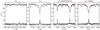 |
Fig. 2 As Fig. 1, but for the FOCES spectrum of KIC 7765135. |
| In the text | |
|
Fig. 3 Observed spectra (dots) of KIC 7985370 and KIC 7765135 (shifted downwards by 0.4) in the Li i λ 6707.8 Å region together with the synthetic spectra (full lines). |
| In the text | |
|
Fig. 4 Abundances found for KIC 7765135 (open circles) and for KIC 7985370 (filled circles) related to the solar ones. |
| In the text | |
|
Fig. 5 Spectral energy distributions (dots) for KIC 7985370 (top panel) and KIC 7765135 (bottom panel). The NextGen synthetic spectrum at Teff = 5800 K scaled to the star distance is overplotted with continuous lines in each box. |
| In the text | |
|
Fig. 6 (U, V) and (W, V) planes of our two young suns. We plotted the average position of each young stellar kinematic group with different symbols. The dotted line in the left panel demarcates the locus of the young-disk population (age < 2 Gyr) in the solar neighborhood, as defined by Eggen (1984, 1989). |
| In the text | |
|
Fig. 7 Cleaned periodograms of the Kepler Q0+Q1+Q2+Q3 time series for KIC 7985370 (upper panel) and KIC 7765135 (lower panel). |
| In the text | |
|
Fig. 8 Kepler light curve with best fit (solid red line, second case-A solution of Table 5) overplotted. The residuals, shown at the top, are ± 2.14 mmag and obviously inhomogeneous from one part of the light curve to another. |
| In the text | |
|
Fig. 9 Determination of the stellar inclination from Kepler photometry. Mean and 68-per-cent confidence interval are indicated by vertical lines (case A only). Dashed: the corresponding marginal distribution for the original data with linear trends removed (case B). |
| In the text | |
|
Fig. 10 Spot intensity related tothe unspotted photosphere. Mean and 68-per-cent confidence interval are indicated by vertical lines (case A only). Dashed: the corresponding marginal distribution for the original data with linear trends removed (case B). |
| In the text | |
|
Fig. 11 All seven marginal distributions (case A) of the spot frequencies. The three frequencies (0.324, 0.340, and 0.350 d-1) seen in the low-resolution Fourier spectrum (Fig. 7) are confirmed by the results of our spot model. |
| In the text | |
|
Fig. 12 Equatorial period of the star. Mean and 68-per-cent confidence interval are indicated by vertical lines (case A only). Dashed: the corresponding marginal distribution for the original data with linear trends removed (case B). |
| In the text | |
|
Fig. 13 Equator-to-pole differential rotation of the star. Mean and 68-per-cent confidence interval are indicated by vertical lines (case A only). Dashed: the corresponding marginal distribution for the original data with linear trends removed (case B). |
| In the text | |
|
Fig. 14 Spot area evolution (case A). Area is in units of the star’s cross-section. Vertical lines mark the boundaries of the Q0 to Q3 quarters of data. A number in parenthesis indicates the spot number. |
| In the text | |
|
Fig. 15 Kepler light curve with best fit (solid red line, case-A solution of Table 7) overplotted. The residuals, shown at the top, are ± 2.35 mmag and obviously inhomogeneous from one part of the light curve to another, hence, the stated ± 2.35 mmag is to be considered an overall average. |
| In the text | |
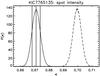 |
Fig. 16 Same as Fig. 10, for KIC 7765135. |
| In the text | |
|
Fig. 17 Marginal distributions of the frequency for all the nine spots. The frequency values group around the two principal frequencies (0.391 and 0.414 d-1) seen already in the Fourier spectrum (Fig. 7), which is the reason for the obvious “beating” phenomenon in Fig. 15 with a period of 40 days. The shortest and the longest frequency are a superposition of two frequencies. |
| In the text | |
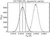 |
Fig. 18 Same as Fig. 12, for KIC 7765135. |
| In the text | |
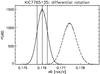 |
Fig. 19 Same as Fig. 13, for KIC 7765135. |
| In the text | |
|
Fig. 20 Same as Fig. 14, for KIC 7765135. Three of the nine spots (# 4, # 7, and # 9) are short-lived ones. Note the change in scale in the upper part! |
| In the text | |
Current usage metrics show cumulative count of Article Views (full-text article views including HTML views, PDF and ePub downloads, according to the available data) and Abstracts Views on Vision4Press platform.
Data correspond to usage on the plateform after 2015. The current usage metrics is available 48-96 hours after online publication and is updated daily on week days.
Initial download of the metrics may take a while.