| Issue |
A&A
Volume 543, July 2012
|
|
|---|---|---|
| Article Number | A127 | |
| Number of page(s) | 10 | |
| Section | Interstellar and circumstellar matter | |
| DOI | https://doi.org/10.1051/0004-6361/201218802 | |
| Published online | 10 July 2012 | |
Polarisation properties of Milky-Way-like galaxies
1 Max-Planck-Institut für Radioastronomie, Auf dem Hügel 69, 53121 Bonn, Germany
e-mail: This email address is being protected from spambots. You need JavaScript enabled to view it.
2 Sydney Institute for Astronomy, School of Physics, The University of Sydney, NSW 2006, Australia
e-mail: This email address is being protected from spambots. You need JavaScript enabled to view it.
3 National Astronomical Observatories, CAS, Jia-20 Datun Road, Chaoyang District, 100012 Beijing, PR China
Received: 10 January 2012
Accepted: 12 June 2012
Abstract
Aims. We study the polarisation properties, magnetic field strength, and synchrotron emission scale-height of Milky-Way-like galaxies in comparison with other spiral galaxies.
Methods. We used our 3D-emission model of the Milky Way Galaxy for viewing the Milky Way from outside at various inclinations in the way that spiral galaxies are observed. We analysed these Milky Way maps with techniques used to obtain the strength of magnetic fields, rotation measures (RMs), and scale-heights of synchrotron emission from observations of resolved galaxies and compared the results with the Milky Way model parameter. We also simulated a large sample of unresolved Milky-Way-like galaxies to study their statistical polarisation properties.
Results. When seen edge-on, the synchrotron emission from the Milky Way has an exponential scale-height of about 0.74 kpc, which is much lower than the values obtained from previous models. We find that current analysis methods overestimate the scale-height of synchrotron emission of galaxies by about 10% at an inclination of 80° and about 40% at an inclination of 70° because of contamination from the disk. The observed RMs for face-on galaxies derived from high-frequency polarisation measurements approximate to the Faraday depths (FDs) when scaled by a factor of two. For edge-on galaxies, the observed RMs are indicative of the orientation of the large-scale magnetic field, but are not closely related with the FDs. Assuming energy equipartition between the magnetic field and particles for the Milky Way results in an average magnetic-field strength that is about twice as high as the intrinsic value for a K factor of 100. The number distribution of the integrated polarisation percentages of a large sample of unresolved Milky-Way-like galaxies peaks at about 4.2% at 4.8 GHz and at about 0.8% at 1.4 GHz. Integrated polarisation angles rotated by 90° align very well with the position angles of the major axes, implying that unresolved galaxies do not have intrinsic RMs.
Conclusions. Simulated maps of the Milky Way Galaxy when viewed from outside at various inclination angles are the basis for a comparison with spiral galaxy maps. They are also helpful to check the accuracy of analysing methods of spiral galaxy observations. Unresolved Milky-Way-like galaxies are ideal background sources to investigate intergalactic magnetic fields. However, at 1.4 GHz they are typically polarised below about 1% and hence a high instrumental purity of future facilities such as the SKA is required to observed them.
Key words: polarization / radio continuum: general / ISM: magnetic fields
© ESO, 2012
1. Introduction
Understanding the role of the magnetic field in spiral galaxies requires to measure its properties and relation to other components of the interstellar medium. The small-scale magnetic fields of the Milky Way Galaxy can be studied in detail. However, properties of the large-scale field are difficult to recover, since the solar system is located within the disk.
Rotation measures (RMs) of polarised background sources are important probes of the large-scale regular magnetic fields in the Milky Way (e.g. Brown et al. 2003, 2007; Taylor et al. 2009; Van Eck et al. 2011). Obtaining a very dense grid of RMs is the major aim of the Magnetism Key Science Project (Beck & Gaensler 2004) that is to be carried out with the future Square Kilometre Array (SKA) and the various pathfinder telescopes such as ASKAP (Johnston et al. 2007) at about 1.4 GHz. At this frequency, however, intrinsic polarisation properties of the various classes of background sources are poorly understood. Recently, Stil et al. (2009) investigated 23 resolved nearby spiral galaxies observed at 4.8 GHz and made a geometric model of the magnetic field to predict the statistical polarisation properties of unresolved galaxies at 1.4 GHz. Simulations with more realistic models are needed to achieve a better insight into the problem.
Polarisation observations have also been widely used to study magnetic fields of resolved nearby galaxies (see Beck 2005, for a review). The RMs are usually obtained from polarisation measurements at short wavelengths, such as λ3.6 cm and λ6 cm, and are believed to indicate the intrinsic galaxy properties. Examples are the low-inclination galaxy NGC 6946 (Beck 2007) and the nearly edge-on galaxy NGC 253 (Heesen et al. 2009). Here it has been presumed that galaxies are optically thin for polarised emission at these wavelengths. However, we have recently found from the Sino-German λ6 cm polarisation survey of the Galactic plane (Sun et al. 2011) that the polarisation horizon is about 4 kpc towards the very inner Galaxy at λ6 cm, just a small portion of the Galaxy. This motivates us to investigate whether RM maps of nearby galaxies correctly show the intrinsic RMs of galaxies.
The Milky Way Galaxy is a typical spiral galaxy, whose magnetic fields have been extensively studied by RMs of pulsars (e.g. Han et al. 2006; Noutsos et al. 2008) and extragalactic sources as mentioned above, as well as by total intensity and polarisation all-sky surveys (e.g. Wolleben et al. 2006; Testori et al. 2008; Page et al. 2007). By taking into account all relevant radio observations available, Sun et al. (2008) and Sun & Reich (2010) proposed 3D-emission models of the Galaxy. Although many parameters need to be refined, the models are the most robust today because they agree with the observations of RMs of extragalactic sources, the all-sky total intensity map at 408 MHz (Haslam et al. 1982), the polarisation map at 22.8 GHz (Gold et al. 2011), and the WMAP thermal emission template (Gold et al. 2009).
Based on the 3D-emission models, we mimic nearby Milky-Way-like galaxies by moving the Galaxy away to various distances and rotate it by arbitrary values. The large sample of simulated Milky-Way-like galaxies allows us to study the statistical properties of their integrated polarisation. We also checked whether the standard assumption of energy equipartition is relevant to estimate the strength of the average magnetic field, and to what extent the inclination of a galaxy affects the determination of its scale-height.
The paper is organised as follows: the simulations of the Milky Way Galaxy and its edge-on view are described in Sect. 2; RMs, scale-height, and energy equipartition for resolved galaxies are investigated in Sects. 3–5. The integrated polarisation properties of a large sample of unresolved Milky-Way-like galaxies are studied in Sect. 6. We summarise our results in Sect. 7.
2. Simulations
2.1. Galactic 3D-emission models
Details of the Galactic 3D-emission models used in this paper were presented by Sun et al. (2008) and Sun & Reich (2010). These models are the basis for the current investigations. They are able to reproduce the large-scale sky distribution of RMs of extragalactic sources as well as total intensity and polarisation all-sky surveys available at several frequencies.
The magnetic field is separated into a large-scale regular field and an isotropic random field. The regular field consists of a disk and a halo component. The halo field is toroidal with opposite signs below and above the Galactic plane. The configuration of the disk field can be either bi-symmetric or axi-symmetric plus reversals following either concentric rings (ASS+RING) or the spiral arms (ASS+ARM). Recent observations of numerous RMs in the Galactic plane by Van Eck et al. (2011) favor the ASS+RING field configuration, which will be used for the present simulations. The local regular magnetic field strength is 2 μG and its scale-height is 1 kpc. The strength of the random field is 3 μG elsewhere.
The 3D-model of the thermal electron density we used is NE2001 (Cordes & Lazio 2002). However, it is essential to adopt the recently revised scale-height of the diffuse ionised gas by Gaensler et al. (2008), otherwise unrealistic parameters result, as discussed by Sun et al. (2008). We therefore increased the scale-height of the thick disk component in NE2001 from 1 kpc to 1.83 kpc and changed the midplane thermal electron density from 3.4 × 10⁻² cm-3 to 1.4 × 10⁻² cm-3. More details were discussed by Sun & Reich (2010). To view the Milky Way Galaxy from outside, we removed all individual features such as clumps and voids, which were included in the NE2001 model. The scale-height of the cosmic-ray electron density was set to 0.8 kpc, and the local density was taken as 6.4 × 10⁻⁵ cm-3. We briefly summarise the main model parameters used for simulations in the present paper in Table 1 and refer to Sun et al. (2008) and Sun & Reich (2010) for details like spatial variations.
Model parameters.
In our Milky Way model, we took the observed local synchrotron emission enhancement into account, which in turn reduced the large extent of the thick disk of previous models (e.g. Phillipps et al. 1981; Beuermann et al. 1985) to account for the observed emission at high latitudes. These earlier models were solely based on the all-sky 408 MHz map and the local synchrotron enhancement was not established at that time. The problem is that available low-frequency absorption data from optically thick H II regions (e.g. Nord et al. 2006; Roger et al. 1999), summarised by Fleishman & Tokarev (1995), did not constrain the 3D-structure of the local enhancement very well. However, meanwhile there are more arguments against the existence of an extended intensive thick disk of the Milky Way. The low percentage polarisation of the WMAP K-band (22.8 GHz) map (Gold et al. 2011) requires a dominating random magnetic field. However, the regular magnetic field is constrained to a few μG by the RMs of extragalactic sources at high latitudes. This in turn means a significant reduction of the cosmic-ray electron density to account for the observed high-latitude synchrotron emission, which requires one to suppress cosmic-ray electron diffusion out of the plane.
The local emission enhancement was modelled as a synchrotron spheroid with uniform emissivity of 1 kpc radius, centred at l = 45°, b = 0° with 560 pc distance from the solar system (Sun & Reich 2010). It is realised in the models by an enhanced cosmic-ray electron density, though one can achieve the same result by increasing the local random magnetic fields (Sun et al. 2008). We kept the local enhancement, which has no influence on the global intensity distribution of the galaxies, as a mark of the position of the solar system.
2.2. Realisation of galaxies from the Milky Way Galaxy
The simulations were performed with the hammurabi code (Waelkens et al. 2009). We revised the code to enable simulations of galaxies in a Cartesian coordinate system in addition to the standard HEALPix system (Górski et al. 2005).
To mimic a nearby spiral galaxy, the Galaxy was put at l = l0, and b = b0 at a distance D, and then rotated by Euler angles (θ1, θ2, θ3). The process is explained in Fig. 1, where a galaxy at xyz is rotated to XYZ. The origin of both coordinate systems corresponds to the centre of the galaxy, and xy or XY indicate the mid-plane of the disk of the galaxy. The Sun is located at x = −8.5 kpc, and y = z = 0. The rotation is accomplished in three steps,
-
around z by θ1;
-
around new x (green line in Fig. 1) by θ2;
-
around Z by θ3.
The inclination (i) of the new Milky-Way-like galaxy is determined by θ1 and θ2 as 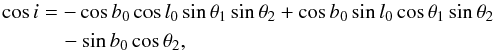 (1)where 0 ≤ θ1 ≤ 2π, and 0 ≤ θ2 ≤ π. In the simulations presented in this paper, we set l0 = 90°, b0 = 0°. The inclination angle of the galaxy is then simplified as cosi = cosθ1cosθ2.
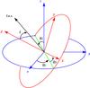 |
Fig. 1 Rotation of the Galaxy from xyz-coordinates to XYZ-coordinates. |
3. Scale-height of the synchrotron emission
3.1. The scale-height of the Milky Way
We simulated the synchrotron emission of the Milky Way Galaxy when seen edge-on at a distance of 5 Mpc. The sampling was chosen to be  to ensure that averaging effects are small. The total intensity of the Milky Way Galaxy seen edge-on at 408 MHz is significantly different from that modelled by Phillipps et al. (1981, their Fig. 8) and Beuermann et al. (1985, their Fig. 9) on the basis of only the 408 MHz all-sky survey (Haslam et al. 1982). The high-latitude emission was attributed to a thick disk component. Phillipps et al. (1981) obtained a huge halo extending in z up to about 10 kpc, and Beuermann et al. (1985) obtained a slightly lower value. We show an edge-on view of the Beuermann et al. (1985) model in comparison with ours in Fig. 2, where the present z-extent is about a factor of two smaller. This difference results from the fact that the current simulations took into account the observed local synchrotron excess as reviewed in Sect. 2.1.
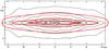 |
Fig. 2 Edge-on view of the Milky Way Galaxy at 408 MHz. The black contours are from the model by Beuermann et al. (1985), and red contours with levels of 10 K, 100 K and 300 K from outside to inside are from the present 3D-model. |
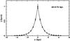 |
Fig. 3 Normalised intensity distribution along z for the Milky Way Galaxy when seen edge-on. The fitted exponential scale-height is z0 = 0.74 kpc. |
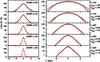 |
Fig. 4 Average intensity distribution (shown by black dots) along z for galaxies observed with a 1′ beam. The projected and smoothed profiles used to obtain the effective HPBW as indicated is shown in the left column. Fits from exponential and Gaussian disks were shown by solid and dotted lines, respectively. |
3.2. The scale-height obtained for inclined galaxies
Dumke et al. (1995, 2000) proposed a scheme to derive the scale-height of the synchrotron emission for highly inclined galaxies. The intensity profile along the major axis is projected to the z axis by scaling the width by a factor cosi. For an edge-on galaxy, the projection results in a delta-function at the centre. The projected profile is then smoothed by using a Gaussian beam corresponding to the angular resolution of the observation. The smoothed profile is fitted by a Gaussian to yield a new half power beam width (HPBW), called the effective beam size. The observed disk profile of a galaxy is commonly assumed to be exponential ( ∝ exp( − | z | /z0, e)) or Gaussian ( ∝  ), which is convolved to the effective beam size. By fitting the newly convolved profile to the observation, the scale-heights (z0, e or z0, g) can be obtained. In this way, both the smoothing effects from the observations and the influence of the inclined disk can be accounted for. This procedure was subsequently used by many authors. Although this method is based on reasonable assumptions, there is no independent verification.
We simulated the 4.8 GHz synchrotron emission from the Galaxy viewed edge-on at a distance of 5 Mpc with a sampling of , made stripe integrations perpendicular to the disk, and normalised the profile with the intensity maximum at z = 0. The result is shown in Fig. 3. The distribution is well fitted by an exponential with a scale-height of 0.74 kpc, which is close to the value of 0.8 kpc for the cosmic-ray electron density in our model (see Table 1). The intrinsic value is thus z = 0.74 kpc, which one expects to obtain from observations at any inclinations and angular resolutions.
We simulated galaxies with inclinations from i = 90° to i = 70° in steps of 5°, and smoothed the total intensity maps to an angular resolution of 1′, which is about that of the Effelsberg 100-m telescope at 10 GHz. Stripe integrations were made in the same way as for the edge-on case shown in Fig. 3 and the results are shown in Fig. 4.
For i = 90° the effective HPBW is 1′ as expected. For lower inclination angles the HPBW gradually broadens, which accounts for the contribution from the disk. For i ≳ 80°, only models with exponential disks yield good fits (Fig. 4). This is expected because the input disk of the model is exponential. For low inclinations, the fits with an exponential or a Gaussian disk are both fairly good for intensities higher than about 10% of the central value (Fig. 4). However, only models with exponential disks reproduce the intrinsic scale-heights reasonably well. The scale-height is overestimated by about 10% at i = 80° and about 40% at i = 70°. The Gaussian disks always produce too large scale-heights. For NGC 253 with  , Heesen et al. (2009) found z = 1.7 ± 0.1 kpc. For this inclination, we obtained a scale-height 15% higher than expected, which exceeds the quoted error, and indicates the inclination limit for the method. For galaxies with inclination angles below i = 70°, the contribution from the disk masks the much fainter halo emission, so that a scale-height determination is not meaningful anymore.
For many galaxies, models with two exponential disks seem to give a better fit. Their typical scale-heights from λ6 cm observations are at the order of 300 pc and 1.8 kpc (e.g. Dumke & Krause 1998; Soida et al. 2011). This is not the case for our Galaxy model, where individual source complexes in the disk are not included. We note that in most cases the difference between one- and two-disk models are based on intensities below about 10% of the central values (e.g. Fig. 6 in Dumke et al. 2000). More galaxies observed with a high signal-to-noise ratios are required for a thorough statistical study.
4. Energy equipartition
The assumption of energy equipartition or minimum energy assumption has been widely used to estimate magnetic fields in galaxies or supernova remnants. Beck (2005) gave a thorough review on this topic and a detailed discussion on its application. We followed Beck & Krause (2005) to calculate the average magnetic field with the observed synchrotron total intensity and spectral index (α), and the so-called K factor, which is the ratio between the proton and electron number density per unit energy. For spiral galaxies, the K factor was traditionally set to 100 (e.g. Niklas & Beck 1997) and more recent evidence favours this value (see e.g. Heesen et al. 2011).
The true average total magnetic field in the disk, which we used in the model, can be represented as 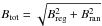 , where the regular field Breg has an exponential shape at radii larger than 5 kpc and a constant value inside, and the random field Bran is homogeneous with a variance of 3 μG (Sun et al. 2008). The radial profile of the total magnetic field calculated this way is shown in Fig. 5.
We simulated the synchrotron emission for an edge-on and a face-on view of the Galaxy. In both cases we assessed the average total magnetic field based on equipartition (Beck & Krause 2005) with a path-length of 20 kpc and 2 kpc, respectively. For K factor, we used the value 100, which is currently the best estimate. The results are shown in Fig. 5. The magnetic field strengths for both views are very similar, because the emission from the disk dominates the total intensity compared to the emission from the halo. At a radius of 8.5 kpc, the field strength is consistent with the value 6 ± 2 μG calculated by Berkhuijsen (see Beck 2001) based on the emission in the plane from the Beuermann et al. (1985) model (see their Fig. 6a).
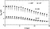 |
Fig. 5 Average total magnetic field estimates based on energy equipartition for an edge-on (open circle) and a face-on (filled circle) view of the Galaxy. The K factor is indicated. The total magnetic field strength of the model is shown by a solid line. |
The magnetic field strength estimated from energy equipartition with a K factor of 100, however, overestimates the true field strength by a factor of nearly 2. To roughly reproduce the intrinsic total magnetic field, the K factor should be about 10 (Fig. 5). However, as already pointed out above, K = 100 seems to be well settled (Heesen et al. 2011). The overestimated magnetic field strength indicates that the cosmic-ray particle energy is about four times higher than the magnetic energy in our model. The energy density of the magnetic field including both regular and random components is  erg cm-3 at R = 8.5 kpc, and correspondingly the energy density of cosmic-ray particles is about ϵCRE = 2.0 × 10⁻¹² erg cm-3. The local total pressure from cosmic rays and magnetic field is
  dyn cm-2. As summarised by Cox (2005), to support the gas against the gravity, the local non-thermal pressure from cosmic rays, magnetic fields and gas motions all together should be about 2.8 × 10⁻¹² dyn cm-2. The dynamic pressure is therefore about 1.6 × 10⁻¹² dyn cm-2, which dominates the pressure from magnetic fields. Recent MHD simulations by Hill et al. (2012) show that the magnetic field does not play an important role in supporting the gas.
Clearly, the equipartition magnetic field strength does not agree with the true value obtained directly from the model. This is not unexpected, because we know that our input model does not satisfy the energy equipartition. In the same sense, it is also very uncertain whether spiral galaxies generally conform to the energy equipartition. It is therefore questionable whether magnetic field estimates based on energy equipartition are reliable.
One may ask if it is possible to use the equipartition value for the magnetic field and adapt the cosmic-ray density accordingly to model the Galaxy. We have tested that and could not reach an agreement with the observations. A higher regular magnetic field will increase the RMs of pulsars and extragalactic sources, which could only be compensated for by decreasing the thermal electron density. The latter, however, has been constrained by pulsar dispersion measures. Increasing the random field component will increase the total synchrotron emission and hence the cosmic-ray electron density must be reduced. This consequently reduces the polarisation intensity. To reproduce the observations, the regular magnetic field has to be increased, which is difficult, as explained at the beginning.
If the Milky Way is not exceptional, the equipartition magnetic field strength estimated for K = 100 might also be lower for other galaxies. The reduction by a factor of two that we found for the Milky Way corresponds to a magnetic energy density decrease by a factor of four and has a large influence on the average magnetic pressure. For example, when equipartition is assumed, the magnetic field energy density clearly dominates the turbulent energy density outside of the inner kpc of NGC 6946 (Beck 2007). This is very puzzling, because the turbulent magnetic field is believed to be connected to turbulent gas motions. When the magnetic energy density is reduced by a factor of four, however, it is almost equal to the turbulent energy density.
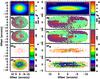 |
Fig. 6 Total intensity (I) at 1.4 GHz, rotation measure (RM) calculated from 4.8 GHz and 8.4 GHz simulations, Faraday depth (FD), and depolarisation maps between 4.8 GHz and 8.4 GHz (DPCX) and between 1.4 GHz and 4.8 GHz (DPLC) for two Milky Way galaxies with inclination angles i = 20° and i = 80°, respectively. |
5. Rotation measures of galaxies
We simulated two samples of galaxies at 4.8 GHz (λ6.25 cm) and 8.4 GHz (λ3.6 cm), which are standard frequencies for nearby galaxy observations. The RM maps of nearby galaxies are mainly calculated from polarisation measurements at these frequencies (e.g. Beck 2007). It is generally assumed that the galaxies are Faraday-thin at these frequencies, which means that the observed polarised emission originates from the same volume. We placed the simulated galaxies at a distance of 5 Mpc, corresponding to a maximum size of about 23′ × 23′, when the galaxies are seen face-on. The resolution or the grid size of the simulations is or about 440 pc, which is comparable to observations and provides some details of the large-scale emission from the galaxies.
We simulated maps for all Stokes parameters and from them calculated polarisation angles (PA) at both frequencies. From the polarisation angle maps, we obtained RM for each individual pixel as  (2)where the subscripts stand for the two bands, e.g. λ = 6.25 cm and λ = 3.6 cm. The nπ-ambiguity of the polarisation angles at these two bands corresponds to an RM of 1194 rad m-2. We assume that n = 0 and the RM values are lower than the ambiguity, which is certainly true except for the centre regions.
The Faraday depth (FD) of a galaxy in rad m-2 is defined as  (3)where ne is the thermal electron density in cm-3 and B ∥ is the magnetic field parallel to the line-of-sight in μG. The integral is calculated along the line-of-sight from the far to the near side of the galaxy. Obviously, FDs are very important to understand the properties of magnetic fields and thermal electron densities. If the synchrotron-emitting medium and the thermal gas are uniformly mixed, one would expect FD = 2RM (e.g. Sokoloff et al. 1998). However, as we will show below, the relation does not hold anymore when the frequency-dependent polarisation horizon is shorter than the size of a galaxy.
The RM and FD maps for a nearly face-on (i = 20°) and a nearly edge-on (i = 80°) galaxy are shown in Fig. 6. In general, both RM and FD maps show the same intensity pattern, which means that RM maps based on observations correctly indicate the orientation of the large-scale field of a galaxy. The field reversals in the Milky Way Galaxy and the opposite sign of the halo magnetic field above and below the Galactic plane are reflected in the RM maps.
The RMs multiplied by a factor of two were compared to the corresponding FDs in Fig. 7. For nearly face-on galaxies (i = 20°) both distributions are basically consistent with each other, although a small amount of scatter is visible. For nearly edge-on galaxies (i = 80°), however, the differences are significant. Strong deviations from FD (Fig. 7) are seen for high FD values originating in the disk. The reason is that the simulated 4.8 GHz and 8.4 GHz polarised emission does not originate from the same volume. The polarisation horizon at 4.8 GHz is smaller than that at 8.4 GHz. Higher-frequency observations are needed to overcome this effect and provide RMs proportional to FDs.
Structure functions (e.g. Sun & Reich 2009) for RMs and FDs were calculated following ![Mathematical equation: \begin{equation} \mathcal{D}\left(\mathbf{\delta\theta}\right) = \left\langle \left[{\rm RM}\left(\mathbf{\theta}\right)- {\rm RM} \left(\mathbf{\theta}+\mathbf{\delta\theta}\right)\right]^2\right\rangle, \end{equation}](/articles/aa/full_html/2012/07/aa18802-12/aa18802-12-eq97.png) (4)where ⟨ ... ⟩ stands for ensemble average and δθ is the angular separation. The results are shown in Fig. 7. The structure functions for RM, when scaled by a factor of two, is equivalent to constantly shifting the structure functions for the original RM upwards along the ordinate axis in Fig. 7. For galaxies with high inclinations, the slopes of the structure functions differ for RMs and FDs, while for low-inclination galaxies RMs mimic FDs quite well after being multiplied by a factor of two.
(4)where ⟨ ... ⟩ stands for ensemble average and δθ is the angular separation. The results are shown in Fig. 7. The structure functions for RM, when scaled by a factor of two, is equivalent to constantly shifting the structure functions for the original RM upwards along the ordinate axis in Fig. 7. For galaxies with high inclinations, the slopes of the structure functions differ for RMs and FDs, while for low-inclination galaxies RMs mimic FDs quite well after being multiplied by a factor of two.
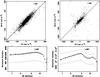 |
Fig. 7 RMs times a factor of two versus FDs (top row). The solid line indicates the expectation for uniformly mixed thermal and synchrotron emission. The structure functions (bottom row) from the FD maps are shown by black dots, those from RM maps and RMs scaled by a factor of two by squares. |
In summary, for face-on galaxies RMs derived from 4.8 GHz and 8.4 GHz polarisation measurements can be safely used to infer magnetic fields after being scaled by a factor of 2. For edge-on galaxies or highly inclined galaxies, however, RMs are only reliable in the outskirts of these galaxies, but still indicate the orientation of the magnetic field direction.
In Fig. 6 we show maps of the depolarisation between the two simulated maps at 4.8 GHz and 8.4 GHz, which show clear differences related to their inclination. For the definition of depolarisation (DPCX) we follow Heesen et al. (2011) as  (5)where β = α − 2 = −3 is the spectral index for brightness temperature. A value of DPCX = 100 means no depolarisation, and DPCX = 0 means total depolarisation. In the depolarisation map for the galaxy with inclination i = 20°, the values exceed 92% everywhere. For the nearly edge-on galaxy with i = 80°, the DPCX along the major axis is small and the values close to the centre are about 40%. Although our model does not include discrete thermal complexes such as H II regions, which are certainly present along the spiral arms, the depolarisation maps show a patchy morphology. This results from the various random magnetic field components along line-of-sights. The highly inclined galaxy NGC 253 with was recently studied by Heesen et al. (2011) using polarisation observations at 4.8 GHz and 8.4 GHz. Their depolarisation map shows similar values as our results, although their distribution of depolarisation patches is more complex than ours. The main reason is the missing discrete source complexes in our model.
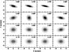 |
Fig. 8 Sample of Milky-Way-like galaxies at 1.4 GHz in total intensity. The inclination angles are marked. The position of the solar system (local enhancement) is indicated by a black dot. The angular resolution is |
We also calculated the depolarisation (DPLC) between 1.4 GHz and 4.8 GHz (Fig. 6). For low-inclination galaxies, DPLC is around 40% within 5′ and there is a slight asymmetry along the minor axis direction, which is caused by the toroidal halo field. We note that some galaxies, for instance NGC 6946, show a clear asymmetric polarisation at frequencies around 1.4 GHz with complete depolarisation towards a large patch (Beck 2007; Heald et al. 2009). This might indicate a more complex halo field configuration than in the Milky Way. A quadrupole field configuration was discussed by Braun et al. (2010), but asymmetries could also be ascribed to some large-scale distortions from a regular configuration. In our Galaxy, discrete large RM or polarisation features exist, for instance the well-pronounced large Fan region (e.g. Wolleben et al. 2006), which are commonly considered to be local. If such regions reside out of the Galactic plane or in the halo, they would make the polarisation properties of our Galaxy asymmetric and thus similar to others. More investigations are needed to improve Galactic emission models.
6. Integrated polarisation properties of Milky-Way-type galaxies
Spiral galaxies are believed to occupy a large part of the polarised radio sources at 1.4 GHz at μJy flux densities (Stil et al. 2007). However, they are difficult to be resolved individually even with instruments such as ASKAP (Johnston et al. 2007) or the future SKA. It is therefore important to investigate the polarisation properties of unresolved spiral galaxies.
We simulated 1000 Milky-Way-like galaxies by randomly setting θ1 and θ2 (see Sect. 2.2) at each of the five frequencies: 1.4 GHz, 2.7 GHz, 4.8 GHz, 8.4 GHz, and 22 GHz. The distance was set to 10 Mpc and the angular resolution to 18″ or 0.87 kpc. We have tried simulations at higher angular resolutions and the results are similar. A sample of Milky-Way-like galaxies at 1.4 GHz is shown in Fig. 8.
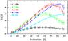 |
Fig. 9 Polarisation percentages of unresolved Milky Way galaxies versus inclination angles at several frequencies as indicated. |
For each object we integrated the I, U and Q maps and obtained the polarisation intensity  and the polarisation percentage Π = PI/I. We binned the data according to their inclination angles with a step interval of 2°. The average percentage polarisation as a function of inclination is shown in Fig. 9.
Face-on galaxies show a low degree of polarisation because of the assumed symmetry of the magnetic field in the disk, which strongly cancels the U and Q components when integrated. This is common for all frequencies (Fig. 9). Faraday effects become highly significant for edge-on galaxies because of the long path-length along the disk emission, which renders the polarisation percentage low. Therefore the maximum polarisation percentage is expected to be at an intermediate level, at about i = 60° at 2.7 GHz, about i = 70° at 4.8 GHz and about i = 80° at 8.4 GHz. The shift stems from the reduction of Faraday depolarisation towards higher frequencies. At low frequencies such as 1.4 GHz, however, Faraday effects are strong irrespective of inclinations, which always yields low polarisation percentages. At high frequencies, the thermal fraction in a galaxy increases, which consequently reduces the polarisation percentage despite reduced Faraday depolarisation and explains the lower percentage polarisation at 22 GHz when compared with those at 8.4 GHz.
The polarisation percentage at 4.8 GHz (Fig. 9) peaks at the same inclination range as that found by Stil et al. (2009) or Stil (2009), who used a geometrical galaxy model. The models by Stil et al. (2009) all predict zero polarisation percentage for edge-on galaxies, which is not found in our simulations. The internal depolarisation for edge-on galaxies was probably overestimated by Stil et al. (2009). In those cases, the polarisation horizon is small (e.g. Sun et al. 2011) and much shorter than the diameter of the disk. However, the disk size was used by Stil et al. (2009) to derive the RM fluctuations, which certainly results in excessively high fluctuation and hence depolarisation. Indeed, most of the edge-on galaxies observed at 4.8 GHz show considerable polarisation percentages (see Fig. 1 in Stil et al. 2009), and agree with our simulations (Fig. 9).
The distribution of polarisation percentages for 1000 simulated galaxies at 1.4 GHz and 4.8 GHz are presented in Fig. 10, which peaks at about 0.8% at 1.4 GHz and 4.2% at 4.8 GHz. In our distributions, the relative number of galaxies at zero polarisation percentage is very small, which is clearly opposite to that in the histograms by Stil et al. (2009, their Fig. 6). This difference is not caused by varying the parameters in the model of Stil et al. (2009), and should be explained in the following way: to ensure a spacial uniform distribution of galaxies, the probability to observe a galaxy at inclination between i and i + di is proportional to sini (e.g. Stil et al. 2009), meaning the relative number of edge-on galaxies is the highest possible. Provided that edge-on galaxies have zero percentage, as modelled by Stil et al. (2009), it follows that there is still a significant number of galaxies at zero percentage in their distributions.
We note that the polarisation percentages can be as high as about 20% in the models by Stil et al. (2009) with varying magnetic field properties. In this paper, we simulated Milky-Way-like galaxies with the same properties as the Galactic interstellar medium, as they were derived from observations (Sun et al. 2008), and simply rotated the Milky Way Galaxy to realise different inclinations. This sample should therefore be considered as a subset of spiral galaxies. In future when more data are available from e.g. GALFACTS (Taylor & Salter 2010), we will aim to represent general galaxies by modifying the Milky Way model accordingly.
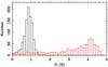 |
Fig. 10 Histogram of polarisation percentages at 1.4 GHz (black) and 4.8 GHz (red) for 1000 simulated Milky Way galaxies. |
The observed polarisation from unresolved galaxies results from averaging the projection of their azimuthal magnetic field components on the plane of the sky. Therefore we expect an alignment between the B-vectors (ΘB) and the position angles of the major axes (Θmajor), which is indeed seen from the present simulations as shown in Fig. 11. This means that polarisation angles of galaxies, when calculated from their integrated emission, do not vary with frequencies, implying that these galaxies do not show intrinsic RMs. This result has already been reported by Stil et al. (2009) from their simulations and is now confirmed. This characteristic makes unresolved spiral galaxies with optically measured position angles ideal background polarised sources to study Galactic and intergalactic large-scale magnetic fields with instruments like the future SKA.
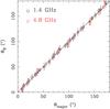 |
Fig. 11 B-vectors (PA + 90°) versus position angles of the major axes from simulated Milky Way galaxies at 1.4 GHz and 4.8 GHz. |
7. Summary
The Milky Way Galaxy is widely considered as a typical spiral galaxy. We used the observationally well-constrained Galactic 3D-emission model (Sun et al. 2008; Sun & Reich 2010) to simulate emission of galaxies by moving the Galaxy to various distances and rotating it by any angle.
In our models, the scale-height of the synchrotron emission from the Milky Way is much lower than that assumed in the early models (Phillipps et al. 1981; Beuermann et al. 1985). At that time, the evidence for the local synchrotron excess was not well determined and therefore not taken into account. We fitted to our Milky Way model, when seen edge-on, an exponential scale-height of 0.74 kpc.
We tested a current analysis method to derive the scale-height of highly inclined galaxies. We found that for Milky Way galaxies the scale-height apparently increases with decreasing inclination. For inclinations higher than 80°, however, the increase is below 10%. The total magnetic field estimate based on the equipartition assumption is about twice that of the Milky Way Galaxy model.
Polarisation observations of highly inclined galaxies when used to derive the distribution of RMs are not reliable for their inner parts. At frequencies of 4.8 GHz or lower, they are not Faraday-thin anymore. The polarised emission from two frequency observations used to calculate RMs originates from different depths. This is also reflected in the slope of the structure functions, which clearly differ for RMs and FDs for galaxies nearly seen edge-on.
We simulated a large sample of distant unresolved galaxies such as will be accessible to the future SKA and its path-finders, and analysed the polarisation properties of this sample for a wide frequency range. This analysis follows that by Stil et al. (2009) of a large spiral galaxy sample based on their model of polarised emission. We qualitatively confirm the Stil et al. (2009) results, where the percentage polarisation drops to zero for face-on galaxies at all frequencies. For edge-on galaxies Stil et al. (2009) found almost no percentage polarisation, while we note a moderate polarisation percentage decrease. The peak percentage polarisation of the galaxy sample peaks at about 4.2% at 4.8 GHz. At 1.4 GHz we find an average percentage polarisations of about 0.8%. We confirm the previous finding by Stil et al. (2009) that unresolved spiral galaxies have a very well aligned polarisation angle in the direction of the galaxies major axis, which makes them ideal sources to study foreground Faraday rotation effects on Mpc-scales.
Acknowledgments
X.S. was supported by the Australian Research Council through grant FL100100114. X.S. acknowledges financial support by the MPG and by Michael Kramer during his stay at MPIfR, where most of this work was done. We thank Patricia Reich and Bryan Gaensler for thorough reading of the manuscript and also the anonymous referee for helpful comments.
References
- Beck, R. 2001, Space Sci. Rev., 99, 243 [NASA ADS] [CrossRef] [Google Scholar]
- Beck, R. 2005, in The Magnetized Plasma in Galaxy Evolution, eds. K. T. Chyzy, K. Otmianowska-Mazur, M. Soida, & R.-J. Dettmar, 193 [Google Scholar]
- Beck, R. 2007, A&A, 470, 539 [NASA ADS] [CrossRef] [EDP Sciences] [Google Scholar]
- Beck, R., & Gaensler, B. M. 2004, New Astron. Rev., 48, 1289 [Google Scholar]
- Beck, R., & Krause, M. 2005, AN, 326, 414 [Google Scholar]
- Beuermann, K., Kanbach, G., & Berkhuijsen, E. M. 1985, A&A, 153, 17 [NASA ADS] [Google Scholar]
- Braun, R., Heald, G., & Beck, R. 2010, A&A, 514, A42 [NASA ADS] [CrossRef] [EDP Sciences] [Google Scholar]
- Brown, J. C., Taylor, A. R., & Jackel, B. J. 2003, ApJS, 145, 213 [NASA ADS] [CrossRef] [Google Scholar]
- Brown, J. C., Haverkorn, M., Gaensler, B. M., et al. 2007, ApJ, 663, 258 [NASA ADS] [CrossRef] [Google Scholar]
- Cordes, J. M., & Lazio, T. J. W. 2002 [arXiv:astro-ph/0207156] [Google Scholar]
- Cox, D. P. 2005, ARA&A, 43, 337 [NASA ADS] [CrossRef] [EDP Sciences] [MathSciNet] [Google Scholar]
- Dumke, M., & Krause, M. 1998, in The Local Bubble and Beyond, eds. D. Breitschwerdt, M. J. Freyberg, & J. Truemper (Berlin: Springer Verlag), IAU Colloq., 166, Lect. Notes Phys., 506, 555 [Google Scholar]
- Dumke, M., Krause, M., Wielebinski, R., & Klein, U. 1995, A&A, 302, 691 [NASA ADS] [Google Scholar]
- Dumke, M., Krause, M., & Wielebinski, R. 2000, A&A, 355, 512 [NASA ADS] [Google Scholar]
- Fleishman, G. D., & Tokarev, Y. V. 1995, A&A, 293, 565 [NASA ADS] [Google Scholar]
- Gaensler, B. M., Madsen, G. J., Chatterjee, S., & Mao, S. A. 2008, PASA, 25, 184 [NASA ADS] [CrossRef] [Google Scholar]
- Gold, B., Bennett, C. L., Hill, R. S., et al. 2009, ApJS, 180, 265 [NASA ADS] [CrossRef] [Google Scholar]
- Gold, B., Odegard, N., Weiland, J. L., et al. 2011, ApJS, 192, 15 [Google Scholar]
- Górski, K. M., Hivon, E., Banday, A. J., et al. 2005, ApJ, 622, 759 [NASA ADS] [CrossRef] [Google Scholar]
- Han, J. L., Manchester, R. N., Lyne, A. G., Qiao, G. J., & van Straten, W. 2006, ApJ, 642, 868 [NASA ADS] [CrossRef] [Google Scholar]
- Haslam, C. G. T., Salter, C. J., Stoffel, H., & Wilson, W. E. 1982, A&AS, 47, 1 [NASA ADS] [Google Scholar]
- Heald, G., Braun, R., & Edmonds, R. 2009, A&A, 503, 409 [NASA ADS] [CrossRef] [EDP Sciences] [Google Scholar]
- Heesen, V., Krause, M., Beck, R., & Dettmar, R. 2009, A&A, 506, 1123 [NASA ADS] [CrossRef] [EDP Sciences] [Google Scholar]
- Heesen, V., Beck, R., Krause, M., & Dettmar, R.-J. 2011, A&A, 535, A79 [NASA ADS] [CrossRef] [EDP Sciences] [Google Scholar]
- Hill, A. S., Joung, M. R., Mac Low, M.-M., et al. 2012, ApJ, 750, 104 [NASA ADS] [CrossRef] [Google Scholar]
- Johnston, S., Bailes, M., Bartel, N., et al. 2007, PASA, 24, 174 [NASA ADS] [CrossRef] [Google Scholar]
- Niklas, S., & Beck, R. 1997, A&A, 320, 54 [NASA ADS] [Google Scholar]
- Nord, M. E., Henning, P. A., Rand, R. J., Lazio, T. J. W., & Kassim, N. E. 2006, AJ, 132, 242 [NASA ADS] [CrossRef] [Google Scholar]
- Noutsos, A., Johnston, S., Kramer, M., & Karastergiou, A. 2008, MNRAS, 386, 1881 [NASA ADS] [CrossRef] [Google Scholar]
- Page, L., Hinshaw, G., Komatsu, E., et al. 2007, ApJS, 170, 335 [NASA ADS] [CrossRef] [Google Scholar]
- Phillipps, S., Kearsey, S., Osborne, J. L., Haslam, C. G. T., & Stoffel, H. 1981, A&A, 103, 405 [NASA ADS] [Google Scholar]
- Roger, R. S., Costain, C. H., Landecker, T. L., & Swerdlyk, C. M. 1999, A&AS, 137, 7 [NASA ADS] [CrossRef] [EDP Sciences] [Google Scholar]
- Soida, M., Krause, M., Dettmar, R.-J., & Urbanik, M. 2011, A&A, 531, A127 [NASA ADS] [CrossRef] [EDP Sciences] [Google Scholar]
- Sokoloff, D. D., Bykov, A. A., Shukurov, A., et al. 1998, MNRAS, 299, 189 [NASA ADS] [CrossRef] [Google Scholar]
- Stil, J. M. 2009, in The Low-Frequency Radio Universe, eds. D. J. Saikia, D. A. Green, Y. Gupta, & T. Venturi, ASP Conf. Ser., 407, 147 [Google Scholar]
- Stil, J., Taylor, A. R., Krause, M., & Beck, R. 2007, in From Planets to Dark Energy: the Modern Radio Universe, 69 [Google Scholar]
- Stil, J. M., Krause, M., Beck, R., & Taylor, A. R. 2009, ApJ, 693, 1392 [NASA ADS] [CrossRef] [Google Scholar]
- Sun, X. H., & Reich, W. 2009, A&A, 507, 1087 [NASA ADS] [CrossRef] [EDP Sciences] [Google Scholar]
- Sun, X. H., & Reich, W. 2010, RAA, 10, 1287 [NASA ADS] [Google Scholar]
- Sun, X. H., Reich, W., Waelkens, A., & Enßlin, T. A. 2008, A&A, 477, 573 [NASA ADS] [CrossRef] [EDP Sciences] [Google Scholar]
- Sun, X. H., Reich, W., Han, J. L., et al. 2011, A&A, 527, A74 [NASA ADS] [CrossRef] [EDP Sciences] [Google Scholar]
- Taylor, A. R., & Salter, C. J. 2010, in ASP Conf. Ser. 438, eds. R. Kothes, T. L. Landecker, & A. G. Willis, 402 [Google Scholar]
- Taylor, A. R., Stil, J. M., & Sunstrum, C. 2009, ApJ, 702, 1230 [NASA ADS] [CrossRef] [Google Scholar]
- Testori, J. C., Reich, P., & Reich, W. 2008, A&A, 484, 733 [NASA ADS] [CrossRef] [EDP Sciences] [Google Scholar]
- Van Eck, C. L., Brown, J. C., Stil, J. M., et al. 2011, ApJ, 728, 97 [NASA ADS] [CrossRef] [Google Scholar]
- Waelkens, A., Jaffe, T., Reinecke, M., Kitaura, F. S., & Enßlin, T. A. 2009, A&A, 495, 697 [NASA ADS] [CrossRef] [EDP Sciences] [Google Scholar]
- Wolleben, M., Landecker, T. L., Reich, W., & Wielebinski, R. 2006, A&A, 448, 411 [NASA ADS] [CrossRef] [EDP Sciences] [Google Scholar]
All Tables
All Figures
|
Fig. 1 Rotation of the Galaxy from xyz-coordinates to XYZ-coordinates. |
| In the text | |
|
Fig. 2 Edge-on view of the Milky Way Galaxy at 408 MHz. The black contours are from the model by Beuermann et al. (1985), and red contours with levels of 10 K, 100 K and 300 K from outside to inside are from the present 3D-model. |
| In the text | |
|
Fig. 3 Normalised intensity distribution along z for the Milky Way Galaxy when seen edge-on. The fitted exponential scale-height is z0 = 0.74 kpc. |
| In the text | |
|
Fig. 4 Average intensity distribution (shown by black dots) along z for galaxies observed with a 1′ beam. The projected and smoothed profiles used to obtain the effective HPBW as indicated is shown in the left column. Fits from exponential and Gaussian disks were shown by solid and dotted lines, respectively. |
| In the text | |
|
Fig. 5 Average total magnetic field estimates based on energy equipartition for an edge-on (open circle) and a face-on (filled circle) view of the Galaxy. The K factor is indicated. The total magnetic field strength of the model is shown by a solid line. |
| In the text | |
|
Fig. 6 Total intensity (I) at 1.4 GHz, rotation measure (RM) calculated from 4.8 GHz and 8.4 GHz simulations, Faraday depth (FD), and depolarisation maps between 4.8 GHz and 8.4 GHz (DPCX) and between 1.4 GHz and 4.8 GHz (DPLC) for two Milky Way galaxies with inclination angles i = 20° and i = 80°, respectively. |
| In the text | |
|
Fig. 7 RMs times a factor of two versus FDs (top row). The solid line indicates the expectation for uniformly mixed thermal and synchrotron emission. The structure functions (bottom row) from the FD maps are shown by black dots, those from RM maps and RMs scaled by a factor of two by squares. |
| In the text | |
|
Fig. 8 Sample of Milky-Way-like galaxies at 1.4 GHz in total intensity. The inclination angles are marked. The position of the solar system (local enhancement) is indicated by a black dot. The angular resolution is |
| In the text | |
|
Fig. 9 Polarisation percentages of unresolved Milky Way galaxies versus inclination angles at several frequencies as indicated. |
| In the text | |
|
Fig. 10 Histogram of polarisation percentages at 1.4 GHz (black) and 4.8 GHz (red) for 1000 simulated Milky Way galaxies. |
| In the text | |
|
Fig. 11 B-vectors (PA + 90°) versus position angles of the major axes from simulated Milky Way galaxies at 1.4 GHz and 4.8 GHz. |
| In the text | |
Current usage metrics show cumulative count of Article Views (full-text article views including HTML views, PDF and ePub downloads, according to the available data) and Abstracts Views on Vision4Press platform.
Data correspond to usage on the plateform after 2015. The current usage metrics is available 48-96 hours after online publication and is updated daily on week days.
Initial download of the metrics may take a while.