| Issue |
A&A
Volume 542, June 2012
GREAT: early science results
|
|
|---|---|---|
| Article Number | L16 | |
| Number of page(s) | 4 | |
| Section | Letters | |
| DOI | https://doi.org/10.1051/0004-6361/201218930 | |
| Published online | 10 May 2012 | |
[12Cii] and [13C ii] 158 μm emission from NGC 2024: Large column densities of ionized carbon
1 I. Physikalisches Institut der Universität zu Köln, Zülpicher Straße 77, 50937 Köln, Germany
e-mail: graf@ph1.uni-koeln.de
2 NASA Ames Research Center, Moffett Field, CA, USA
3 Max-Planck-Institut für Radioastronomie, Auf dem Hügel 69, 53121 Bonn, Germany
4 Max-Planck-Institut für Sonnensystemforschung, Max-Planck-Straße 2, 37191 Katlenburg-Lindau, Germany
5 Deutsches Zentrum für Luft- und Raumfahrt, Institut für Planetenforschung, Rutherfordstraße 2, 12489 Berlin, Germany
6 Institut für Optik und Atomare Physik, Technische Universität Berlin, Hardenbergstraße 36, 10623 Berlin, Germany
Received: 31 January 2012
Accepted: 1 March 2012
Context. We analyze the NGC 2024 Hii region and molecular cloud interface using [12Cii] and [13Cii] observations.
Aims. We attempt to gain insight into the physical structure of the interface layer between the molecular cloud and the Hii region.
Methods. Observations of [12Cii] and [13Cii] emission at 158 μm with high spatial and spectral resolution allow us to study the detailed structure of the ionization front and estimate the column densities and temperatures of the ionized carbon layer in the photon-dominated region.
Results. The [12Cii] emission closely follows the distribution of the 8 μm continuum. Across most of the source, the spectral lines have two velocity peaks similar to lines of rare CO isotopes. The [13Cii] emission is detected near the edge-on ionization front. It has only a single velocity component, which implies that the [12Cii] line shape is caused by self-absorption. An anomalous hyperfine line-intensity ratio observed in [13Cii] cannot yet be explained.
Conclusions. Our analysis of the two isotopes results in a total column density of N(H) ≈ 1.6 × 1023 cm-2 in the gas emitting the [Cii] line. A large fraction of this gas has to be at a temperature of several hundred K. The self-absorption is caused by a cooler (T ≤ 100 K) foreground component containing a column density of N(H) ≈ 1022 cm-2.
Key words: ISM: atoms / ISM: clouds / ISM: individual objects: NGC 2024 / photon-dominated region (PDR)
© ESO, 2012
1. Introduction
NGC 2024 is a well-studied star forming region at a distance of 415 pc (Anthony-Twarog 1982) in the Orion B complex. The source consists of a dense (n ≈ 106 cm-3, Schulz et al. 1991), narrow (≈1′), north-south extended molecular cloud with an embedded Hii region (Krügel et al. 1982; Crutcher et al. 1986; Barnes et al. 1989), which extends several arcminutes beyond the molecular ridge in the east-west direction. The molecular material in front of the Hii region is seen as a prominent dust lane in the optical. Both OH (Barnes et al. 1989) and H2CO (Crutcher et al. 1986) absorption line measurements relative to the radio continuum indicate that this material is at a radial velocity of vLSR ≈ 9 km s-1. The bulk of the molecular gas behind the Hii region is found at vLSR ≈ 11 km s-1 from observations of e.g. optically thin CO (Mauersberger et al. 1992; Graf et al. 1993; Emprechtinger et al. 2009; Buckle et al. 2010) or HCO+ (Richer et al. 1989) lines. In the south of the Hii region, a sharp ionization front delineates the boundary between the ionized and the molecular gas (e.g. MSX data in Watanabe & Mitchell 2008). This ionization front is seen edge-on in the south of the Hii region, but probably also extends north in a face-on geometry along both the foreground and the background parts of the cloud.
The velocity dispersion in each of the two main parts of the cloud is small ΔvLSR ≈ 2 km s-1, which leads to a conspicuous double-peaked line shape in many molecular emission lines. Detailed modeling of these lines (Graf et al. 1993; Emprechtinger et al. 2009) results in H2 column densities of a few times 1022 cm-2 for the foreground component and 1–2 × 1023 cm-2 for the background component. Gas temperatures are found to be around 70 K in the background and around 30 K in the foreground, with a likely increase near the Hii region interface.
In this Letter, we present [Cii] maps of an area near the ionization front. Our analysis concentrates on the physical properties implied by the strong [13Cii] emission detected.
2. Observations
We observed the  fine structure transition of ionized carbon (C+) at 1900.5369 GHz (157.7 μm) (Cooksy et al. 1986) toward the NGC 2024 (Orion B) molecular cloud. The measurements were made on Nov. 8, 2011 using the German REceiver for Astronomy at Terahertz frequencies (GREAT)1 (Heyminck et al. 2012) on the Stratospheric Observatory For Infrared Astronomy (SOFIA; Young et al. 2012).
The receiver noise temperature during the observations was approximately 4000 K (SSB). With a zenith opacity of 0.03–0.07, the system temperature was lower than 4500 K (SSB). The beam size was 16′′. The velocity resolution before smoothing was 33 m/s.
We mapped a 192″ × 144″ area in total power on-the-fly mode. Both the sampling distance along the scan direction and the scan spacing were 6″. The map was centered on (α,δ) = ( ) (J2000) using an off-position at (
 ,
,  ). According to Jaffe et al. (1994) and confirmed by a comparison measurement to a second, far-away off-position, no [Cii] emission could be detected at this position.
The measurements were calibrated using the procedure outlined in Guan et al. (2012). Instead of the main beam efficiency of 0.51 (Heyminck et al. 2012), we used a value of 0.58 to account for the non-negligible coupling of the first side lobes to an extended source, as derived from a model of the diffraction pattern. A linear baseline was subtracted from each spectrum.
3. Results
Figure 1 shows the measured [Cii] intensity distribution integrated over the velocity interval 5–15 km s-1. The emission agrees remarkably well with the 8 μm MSX data (Price et al. 2001; Watanabe & Mitchell 2008), which traces the UV-heated dust in the interface between the Hii region and the molecular cloud. Only the embedded MSX source just north of the map center is not very prominent in the [Cii] data. The emission peaks along the southern rim of the Hii region, where the interface is seen edge-on in a sharp ionization front.
The intensity distribution does not reflect the distribution of the molecular material located in a roughly north-south elongated molecular ridge – outlined by the FIR peaks in Fig. 1.
Averaged over a 60′′ diameter, we obtain a peak surface brightness of 4.4 × 10⁻³ erg cm-2 s-1 sr-1, in reasonable agreement with KAO and ISO data (Jaffe et al. 1994; Giannini et al. 2000).
3.1. [13C ii] distribution
With a velocity span of ± 100 km s-1, the spectra also cover the three hyperfine structure components of the [13Cii] transition (vLSR-offsets −65.2, 11.2, 63.2 km s-1, Cooksy et al. 1986) (Fig. 3). If we co-add the velocity ranges [−60, −50], [19,25], and [70,80] km s-1 (taking into account the systemic velocity), we find emission with a similar spatial distribution as the main isotope (Fig. 1).
The [13Cii] emission is only prominent in a crescent-shaped area following the edge-on ionization front, where column densities are highest. The peak emission coincides with the [12Cii] emission maximum, but the [13Cii] intensity falls off more rapidly, both to the Hii region side (north) and to the molecular cloud side (south). The FWHM of the [13Cii] emission zone is ≈ 1′, corresponding to a linear size of ≈0.1 pc.
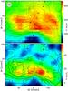 |
Fig. 1 Top: integrated (5–15 km s-1) [Cii] intensity map of NGC 2024 (color code). Comparison data: MSX Band A (8.28 μm) (contours), 6 cm continuum peaks (triangles) (Crutcher et al. 1986), 1.3 mm continuum emission clumps FIR2 to FIR6 (squares) (Mezger et al. 1988), and embedded infrared point sources IRS2 (Grasdalen 1974) and IRS3 (Barnes et al. 1989) (stars). Bottom: overlay of the [13Cii] (color coded) and the [12Cii] integrated intensities (contours: 100 K km s-1 to 625 K km s-1 in steps of 75 K km s-1). The [13Cii] map has been smoothed to a resolution of 25″. The dashed box outlines the area of strong emission that was used in the analysis of Sect. 4. |
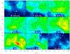 |
Fig. 2 [12Cii] channel maps of 1 km s-1 wide velocity channels spaced by 1 km s-1. Panels are labeled by their center velocity. The markers denote the positions of the clumps FIR2 to FIR6 (Mezger et al. 1988). Contour levels are from 10 K km s-1 to 150 K km s-1 in steps of 20 K km s-1. |
3.2. [12C ii] channel maps
The [Cii] emission is separated into two distinct velocity components, which show up as two peaks in most spectra (Fig. 3). Figure 2 presents channel maps of 1 km s-1 wide velocity bins ranging from 6 km s-1 to 14 km s-1. The maps clearly show the two main velocity peaks, which are predominant throughout most of the source. The low velocity peak dominates the 8–9 km s-1 panels, the high velocity peak being clearly visible at 11 and 12 km s-1. The local minimum in the 10 km s-1 velocity bin around FIR5 coincides with the peak of the integrated intensity map (Fig. 1).
There appears to be an anticorrelation between the low velocity peak and the high velocity peak. The relatively high intensities found at 9 km s-1 west of FIR2 to FIR4 and east of FIR5 correspond to areas of weak emission at 12–13 km s-1.
4. Discussion
For the data analysis, the interpretation of the two velocity peaks of the spectra is crucial. Although the [Cii] peaks – at velocities of ~8.4 km s-1 and ~12 km s-1 – are slightly offset from the two emission components in the optically thin lines of very rare CO isotopes (9.2 km s-1 and 11.2 km s-1, Graf et al. 1993), it seems reasonable to assume that the [Cii] line may also be caused by two emission components and not by self-absorption. The [13Cii] measurement allows us to clearly distinguish between these two possibilities.
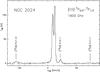 |
Fig. 3 Spectrum averaged over the area outlined in Fig. 1 with marks indicating the predicted velocities of the [13Cii] hyperfine components (Cooksy et al. 1986). |
4.1. [13C ii] spectrum
To obtain a high signal-to-noise spectrum to analyze the isotopic line, we averaged the spectra within a rectangular area encompassing the peak of the [13Cii] emission (marked by a dashed box in Fig. 1). The resulting spectrum is shown in Fig. 3. In Fig. 4, we compare the line profile of the [12Cii] line to the three hyperfine satellites of [13Cii].
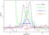 |
Fig. 4 Spectrum of Fig. 3 replotted on a common vLSR scale and overlaid by the model fit (see text and Table 1). The dashed line marks the center velocity of the [12Cii] background component. Horizontal bars indicate the uncertainty in the rest frequencies. The [12Cii] has been divided by ten. |
It is immediately obvious that the isotopic line only shows a single peak. Thus, either a) only one of the two velocity components seen in [12Cii] has a sufficiently high column density to produce measurable [13Cii] emission, or b) the shape of the [12Cii] is produced by a warm broad background component shadowed by a narrow cooler foreground component. Explanation a) would imply that there is an error in the rest frequencies of ≳ 10 MHz, clearly beyond the confidence limits of Cooksy et al. (1986) and in contrast to the good agreement found in recent HIFI measurements toward the Orion bar (Ossenkopf et al. 2011). Thus, if we accept the rest frequencies to their published accuracy, we are forced to the conclusion that the [12Cii] line profile is caused by self-absorbed strong background emission centered at vLSR ≈ 10 km s-1.
Self-absorption in the [12Cii] line offers a quite natural explanation of the anticorrelation observed in the spatial distribution of the two velocity peaks: a velocity shift of the absorbing component with respect to the background component shifts the observed line intensity from one velocity peak to the other.
That the highest contrast between the 10 km s-1 dip and the 8 km s-1 and 12 km s-1 peaks is found in an area of known strong foreground absorption (Crutcher et al. 1986; Barnes et al. 1989) also strengthens this interpretation. Radio recombination lines of carbon (Krügel et al. 1982, and reference therein) are also mostly near 10 km s-1.
The discrepancy between the CO velocities and the self-absorbed [Cii] emission indicates that the simple source model with only two velocity components may underestimate the kinematic complexity of the source.
4.2. Hyperfine line ratios
Figure 4 includes the result of a five-component Gaussian fit to the spectrum. The first two components model the main isotope (fit not shown in Fig. 4) as an emissive and an absorptive component. The remaining three components fit the three hyperfine lines, where the line width is kept fixed and equal to the width of the broad background component. Table 1 lists the fit results and compares the parameters of the [13Cii] hyperfine satellites to the literature values.
For the two stronger hyperfine components, the velocities are within 0.5 km s-1 (3 MHz) of the predicted values. The signal-to-noise ratio of the F = 1 → 1 component is too low to make a firm statement. The predicted line strength ratio, however, is not reproduced by our measurement. The (F = 2 → 1)/(F = 1 → 0) intensity ratio should be 1.25, but is found to be 1.9. A similar discrepancy was also found by Ossenkopf et al. (2011).
Obviously it cannot be ruled out that an as yet unknown emission line may coincide with the F = 2 → 1 line, leading to excess emission at this velocity. However, strong spectral lines at these wavelengths are so rare that this seems highly unlikely. At the moment, we can only speculate that the anomalous hyperfine ratio may be due to some non-LTE excitation mechanism, possibly caused by hyperfine-selective radiative pumping by emission lines of the main isotope at shorter wavelengths.
4.3. Physical conditions
The integrated intensity in the three hyperfine components adds up to 52 K km s-1, which – in the high density limit (n > 3000 cm-3) – converts into a column density N(13C+) = 2.6 × 1017 cm-2 (Crawford et al. 1985). Assuming standard abundance ratios2, this corresponds to N(12C+) = 1.6 × 1019 cm-2 and a total hydrogen column density of N(H) = 1.6 × 1023 cm-2 in the gas emitting the [Cii] lines, if all the carbon is ionized.
Owing to the foreground absorption, the intrinsic [12Cii] emission is not constrained well. The background emission line component requires temperatures of several 100 K, with 165 K being a hard lower limit3. For a gas temperature of e.g. 400 K, the [12Cii] line would be almost optically thick (τ ≈ 2.4) with an intrinsic line temperature of TMB([12Cii], background) ≈ 325 K.
Standard spherical photon-dominated region (PDR) models (Störzer et al. 1996; Röllig et al. 2006) of even the most extreme single clumps fall short by about one order of magnitude of reproducing this high line intensity and large column density of ionized carbon. It is plausible that the edge-on geometry of the ionization front may significantly boost the total column density. Thus, an equivalent of ten extreme clumps would be required to model the observed emission. Similarly, in a clumpy PDR model (Cubick et al. 2008), where the amount of material exposed to UV radiation is drastically higher, the predicted [Cii] emission is much stronger. For instance, a typical model4 with a total mass within the beam of 1 M⊙, a radiation field of χ = 103 and an average density of 106 cm-3 can produce the observed [13Cii] intensity. These values correspond to a hydrogen column density of ≈ 1023 cm-2, in agreement with the above estimate.
With the absorption dip reaching down to 53 K (Fig. 4), the temperature in the foreground gas is limited to TFG ≤ 90 K5. The optical depth derived for the foreground gas is τFG ≥ 1, where the exact value depends on the assumptions made about the temperatures. If we accept an intrinsic main beam brightness temperature of 325 K for the background component, the column density of ionized carbon in the absorbing layer needs to be N(C+) ≥ 1018 cm-2 for any gas temperature above 40 K.
5. Conclusions
We have observed both [12Cii] and [13Cii] emission toward NGC 2024. The spatial distribution of the emission follows the 8 μm continuum emission, tracing the interface between the Hii region and the molecular cloud. The isotopic line emission detected from an area near the ionization front implies that:
-
the double-peaked spectrum of the [12Cii] line is due to strong background emission absorbed by cooler foreground gas at the same velocity;
-
the kinematic signature of the ionized gas differs from that of the molecular gas as traced by rare isotopes of CO;
-
the total hydrogen column density of warm gas at several hundred Kelvin traced by the [Cii] emission amounts to ≥ 1023 cm-2, suggesting that the interface is highly clumpy;
-
the strong foreground absorption implies a hydrogen column density ≥ 1022 cm-2 of gas at temperatures below 100 K;
-
The measured intensity ratio of the hyperfine components does not match the theoretical value, suggesting that there is some contribution from a non-LTE excitation effect
Owing to the Rayleigh-Jeans correction, the peak TMB of 125 K (Fig. 4) requires gas temperatures of ≥ 165 K.
Acknowledgments
We thank Volker Ossenkopf and Markus Röllig for useful discussions. We also thank the SOFIA engineering and operations teams whose tireless support and good-spirit teamwork has been essential for the GREAT accomplishments during Early Science, and say Herzlichen Dank to the DSI telescope engineering team. This work is based on observations made with the NASA/DLR Stratospheric Observatory for Infrared Astronomy. SOFIA Science Mission Operations are conducted jointly by the Universities Space Research Association, Inc., under NASA contract NAS2-97001, and the Deutsches SOFIA Institut under DLR contract 50 OK 0901.
References
- Anthony-Twarog, B. J. 1982, AJ, 87, 1213 [NASA ADS] [CrossRef] [Google Scholar]
- Barnes, P. J., Crutcher, R. M., Bieging, J. H., Storey, J. W. V., & Willner, S. P. 1989, ApJ, 342, 883 [NASA ADS] [CrossRef] [Google Scholar]
- Buckle, J. V., Curtis, E. I., Roberts, J. F., et al. 2010, MNRAS, 401, 204 [NASA ADS] [CrossRef] [Google Scholar]
- Cooksy, A. L., Blake, G. A., & Saykally, R. J. 1986, ApJ, 305, L89 [NASA ADS] [CrossRef] [Google Scholar]
- Crawford, M. K., Genzel, R., Townes, C. H., & Watson, D. M. 1985, ApJ, 291, 755 [NASA ADS] [CrossRef] [Google Scholar]
- Crutcher, R. M., Henkel, C., Wilson, T. L., Johnston, K. J., & Bieging, J. H. 1986, ApJ, 307, 302 [NASA ADS] [CrossRef] [Google Scholar]
- Cubick, M., Stutzki, J., Ossenkopf, V., Kramer, C., & Röllig, M. 2008, A&A, 488, 623 [NASA ADS] [CrossRef] [EDP Sciences] [Google Scholar]
- Emprechtinger, M., Wiedner, M. C., Simon, R., et al. 2009, A&A, 496, 731 [NASA ADS] [CrossRef] [EDP Sciences] [Google Scholar]
- Giannini, T., Nisini, B., Lorenzetti, D., et al. 2000, A&A, 358, 310 [NASA ADS] [Google Scholar]
- Graf, U. U., Eckart, A., Genzel, R., et al. 1993, ApJ, 405, 249 [NASA ADS] [CrossRef] [Google Scholar]
- Grasdalen, G. L. 1974, ApJ, 193, 373 [NASA ADS] [CrossRef] [Google Scholar]
- Guan, X., Stutzki, J., Graf, U. U., et al. 2012, A&A, 542, L4 [Google Scholar]
- Heyminck, S., Graf, U. U., Güsten, R., et al. 2012, A&A, 542, L1 [NASA ADS] [CrossRef] [EDP Sciences] [Google Scholar]
- Jaffe, D. T., Zhou, S., Howe, J. E., et al. 1994, ApJ, 436, 203 [NASA ADS] [CrossRef] [Google Scholar]
- Krügel, E., Thum, C., Pankonin, V., & Martin-Pintado, J. 1982, A&AS, 48, 345 [NASA ADS] [Google Scholar]
- Mauersberger, R., Wilson, T. L., Mezger, P. G., Gaume, R., & Johnston, K. J. 1992, A&A, 256, 640 [NASA ADS] [Google Scholar]
- Mezger, P. G., Chini, R., Kreysa, E., Wink, J. E., & Salter, C. J. 1988, A&A, 191, 44 [NASA ADS] [Google Scholar]
- Ossenkopf, V., Röllig, M., Fuente, A., et al. 2011, in IAU Symp. 280, 280 [Google Scholar]
- Price, S. D., Egan, M. P., Carey, S. J., Mizuno, D. R., & Kuchar, T. A. 2001, AJ, 121, 2819 [NASA ADS] [CrossRef] [Google Scholar]
- Richer, J. S., Hills, R. E., Padman, R., & Russell, A. P. G. 1989, MNRAS, 241, 231 [NASA ADS] [CrossRef] [Google Scholar]
- Röllig, M., Ossenkopf, V., Jeyakumar, S., Stutzki, J., & Sternberg, A. 2006, A&A, 451, 917 [NASA ADS] [CrossRef] [EDP Sciences] [Google Scholar]
- Schulz, A., Güsten, R., Zylka, R., & Serabyn, E. 1991, A&A, 246, 570 [NASA ADS] [Google Scholar]
- Störzer, H., Stutzki, J., & Sternberg, A. 1996, A&A, 310, 592 [NASA ADS] [Google Scholar]
- Watanabe, T., & Mitchell, G. F. 2008, AJ, 136, 1947 [NASA ADS] [CrossRef] [Google Scholar]
- Young, E. T., Becklin, E. E., Marcum, J. M., et al. 2012, ApJ, 749, L17 [NASA ADS] [CrossRef] [Google Scholar]
All Tables
All Figures
|
Fig. 1 Top: integrated (5–15 km s-1) [Cii] intensity map of NGC 2024 (color code). Comparison data: MSX Band A (8.28 μm) (contours), 6 cm continuum peaks (triangles) (Crutcher et al. 1986), 1.3 mm continuum emission clumps FIR2 to FIR6 (squares) (Mezger et al. 1988), and embedded infrared point sources IRS2 (Grasdalen 1974) and IRS3 (Barnes et al. 1989) (stars). Bottom: overlay of the [13Cii] (color coded) and the [12Cii] integrated intensities (contours: 100 K km s-1 to 625 K km s-1 in steps of 75 K km s-1). The [13Cii] map has been smoothed to a resolution of 25″. The dashed box outlines the area of strong emission that was used in the analysis of Sect. 4. |
| In the text | |
|
Fig. 2 [12Cii] channel maps of 1 km s-1 wide velocity channels spaced by 1 km s-1. Panels are labeled by their center velocity. The markers denote the positions of the clumps FIR2 to FIR6 (Mezger et al. 1988). Contour levels are from 10 K km s-1 to 150 K km s-1 in steps of 20 K km s-1. |
| In the text | |
|
Fig. 3 Spectrum averaged over the area outlined in Fig. 1 with marks indicating the predicted velocities of the [13Cii] hyperfine components (Cooksy et al. 1986). |
| In the text | |
|
Fig. 4 Spectrum of Fig. 3 replotted on a common vLSR scale and overlaid by the model fit (see text and Table 1). The dashed line marks the center velocity of the [12Cii] background component. Horizontal bars indicate the uncertainty in the rest frequencies. The [12Cii] has been divided by ten. |
| In the text | |
Current usage metrics show cumulative count of Article Views (full-text article views including HTML views, PDF and ePub downloads, according to the available data) and Abstracts Views on Vision4Press platform.
Data correspond to usage on the plateform after 2015. The current usage metrics is available 48-96 hours after online publication and is updated daily on week days.
Initial download of the metrics may take a while.