| Issue |
A&A
Volume 542, June 2012
|
|
|---|---|---|
| Article Number | A63 | |
| Number of page(s) | 8 | |
| Section | Astronomical instrumentation | |
| DOI | https://doi.org/10.1051/0004-6361/201218833 | |
| Published online | 07 June 2012 | |
The wideband backend at the MDSCC in Robledo
A new facility for radio astronomy at Q- and K-bands
1 Centro de Astrobiología (INTA-CSIC), Ctra. M-108, km. 4, Torrejón de Ardoz 28850, Madrid, Spain
e-mail: This email address is being protected from spambots. You need JavaScript enabled to view it.
2 Instituto Nacional de Técnica Aeroespacial, Ctra. M-108, km. 4, Torrejón de Ardoz 28850, Madrid, Spain
3 Madrid Deep Space Communications Complex, Ctra. M-531, km. 7, Robledo de Chavela 28294, Madrid, Spain
4 Jet Propulsion Laboratory, California Institute of Technology, 4800 Oak Grove Drive, Pasadena, CA 91109, USA
Received: 17 January 2012
Accepted: 15 March 2012
Abstract
Context. The antennas of NASA’s Madrid Deep Space Communications Complex (MDSCC) in Robledo de Chavela are available as single-dish radio astronomical facilities during a significant percentage of their operational time. Current instrumentation includes two antennas of 70 and 34 m in diameter, equipped with dual-polarization receivers in K (18–26 GHz) and Q (38–50 GHz) bands, respectively. Until mid-2011, the only backend available in MDSCC was a single spectral autocorrelator, which provides bandwidths from 2 to 16 MHz. The limited bandwidth available with this autocorrelator seriously limited the science one could carry out at Robledo.
Aims. We have developed and built a new wideband backend for the Robledo antennas, with the objectives (1) to optimize the available time and enhance the efficiency of radio astronomy in MDSCC; and (2) to tackle new scientific cases that were impossible to investigate with the existing autocorrelator.
Methods. The features required for the new backend include (1) a broad instantaneous bandwidth of at least 1.5 GHz; (2) high-quality and stable baselines, with small variations in frequency along the whole band; (3) easy upgradability; and (4) usability for at least the antennas that host the K- and Q-band receivers.
Results. The backend consists of an intermediate frequency (IF) processor, a fast Fourier transform spectrometer (FFTS), and the software that interfaces and manages the events among the observing program, antenna control, the IF processor, the FFTS operation, and data recording. The whole system was end-to-end assembled in August 2011, at the start of commissioning activities, and the results are reported in this paper. Frequency tunings and line intensities are stable over hours, even when using different synthesizers and IF channels; no aliasing effects have been measured, and the rejection of the image sideband was characterized.
Conclusions. The new wideband backend fulfills the requirements and makes better use of the available time for radio astronomy, which opens new possibilities to potential users. The first setup provides 1.5 GHz of instantaneous bandwidth in a single polarization, using 8192 channels and a frequency resolution of 212 kHz; upgrades under way include a second FFTS card, and two high-resolution cores providing 100 MHz and 500 MHz of bandwidth, and 16 384 channels. These upgrades will permit simultaneous observations of the two polarizations with instantaneous bandwidths from 100 MHz to 3 GHz, and spectral resolutions from 7 to 212 kHz.
Key words: instrumentation: miscellaneous / instrumentation: spectrographs / techniques: spectroscopic / ISM: lines and bands / ISM: molecules / radio lines: general
© ESO, 2012
1. Radio astronomy activity in Robledo
The NASA Deep Space Network1 (DSN) is the international network of antennas used to support tracking and operations activities of space missions usually beyond the Earth orbits. The DSN currently consists of three complexes located at Goldstone (USA), Canberra (Australia), and Robledo de Chavela (Spain). Each complex hosts several sensitive, large-aperture antennas, whose diameters are between 26 and 70 m.
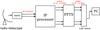 |
Fig. 1 Concept diagram of the signal path from the antenna receiver (HEMT) through the backend. The first stage of the backend is the IF processor, followed by the FFT spectrometer. Finally, data are processed and recorded on a dedicated PC (see text). |
The Robledo complex, namely Madrid Deep Space Communications Complex (MDSCC), has six of these antennas. A fraction of the operational time of the MDSCC antennas are routinely used for radio astronomical observations. In addition to its use as a VLBI station through the European VLBI Network (EVN), the antennas are usable as single-dish radio telescopes by means of two different programs, the “Guest Observer” program, which involves all the DSN antennas and is managed directly by JPL, and the so-called “Host Country” radio astronomy program, which is a guaranteed time program for Spanish astronomers managed by INTA (Instituto Nacional de Técnica Aeroespacial). All six antennas and their corresponding receivers are available, although two instruments are actively used for radio astronomy: the DSS-63 antenna, 70 m in diameter, equipped with a K-band (18–26 GHz) receiver; and the DSS-54 antenna, 34 m in diameter, equipped with a Q-band (38–50 GHz) receiver. Table 1 summarizes the main technical characteristics of these two antennas.
The two major antennas at MDSCC, Robledo.
The two bands mentioned in Table 1 include several important molecular lines, and the angular resolution of both antennas are similar (slightly above 40′′, depending on the observing frequency). Single-dish radio astronomy at MDSCC can address a wide variety of scientific categories, such as the studies of the interstellar and circumstellar media, star formation and evolution, and solar system bodies (Gómez et al. 2006; Suárez et al. 2007; Busquet et al. 2009; Horiuchi et al. 2010). Until mid 2011, the only backend available at MDSCC was an autocorrelator, which provides excellent spectral resolution, (as low as 5 kHz) but instantaneous bandwidths of 2, 4, 8, and 16 MHz. This limitation seriously affected the possible science cases; there are no practical possibilities to perform, for example, spectral surveys, simultaneous line observations, extragalactic astronomy, or the observations of a single spectral line in sources that have a wide velocity range of emission.
Aiming to overcome the bandwidth limitation problem, we have started in 2009 the design and construction of a new complete backend system for its use in the Robledo antennas. The backend was end-to-end assembled by mid-2011, when the commissioning tests of the first setup started. This paper reports the main features of the new backend, some astronomical results of the commissioning, and prospects for future upgrades.
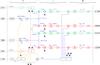 |
Fig. 2 Block diagram of the IF processor. Input polarizations are marked by red and green colors. The signals are divided into two channels, LO and HI, for each polarization, providing four output channels at base band. |
2. The new wideband backend
2.1. Aims and features
The new backend was conceived with the objectives to optimize the use of available time for single-dish radio astronomy in MDSCC and to tackle new scientific cases which was impossible to do using the current autocorrelator. The current high sampling rate of commercially available analog-to-digital converters (ADCs) together with the high power of field programable gate array (FPGA) chips allowed us to consider a complete backend able to process several GHz of instantaneous bandwidth. Large bandwidth spectrometers have been developed at several radio telescopes since the early 2000s. Also, high-performance electronics are now commercially available, ensuring reliable intermediate frequency (IF) processing, maintaining the quality of such large bandwidths.
Two other features are required for the backend. First, it has to be easily upgradeable to permit enhancements without the need to discard already acquired/built components. Second, the new backend has to be useful for the two major receivers that operate in single-dish radio astronomy at the MDSCC (the Q- and K-band receivers already mentioned).
Figure 1 sketches the concept of the backend. The fist stage is the radio signal reception, by means of the K- or Q-band receivers. The K-band frequency range goes from 18 to 26 GHz, while the Q-band receiver is sensitive from 38 to 50 GHz; the Q-band signal is mixed to a local oscillator at 62 GHz within the receiver, which results in a mirrored band transport to the range 12 to 24 GHz. Therefore, a backend usable for both receivers should be able to process signals from 12 to 26 GHz in two polarizations. The two-polarization radio signal (RF in Fig. 1) goes then to the first part of the backend, namely the IF processor. The IF processor splits each polarization radio signal into two channels and downconverts the resulting four channels, giving four base band (BB) analog outputs from 0 to 1.5 GHz. The second step of the backend is a fast Fourier transform spectrometer (FFTS), which digitizes and samples the BB signals. The final step is to manage and record the data, which is done through a program on a dedicated PC.
2.2. The IF processor
The IF processor was designed and built at the INTA’s radar laboratory, with the exception of several semi-rigid cables, which have been assembled at JPL.
Figure 2 depicts a block diagram of the IF processor, while Table 2 summarizes its specifications. Two input signals are shown, which correspond to both polarizations of the radio signal. Each polarization is then split into two parts, which are meant as low- and high-frequency channels (LO and HI, respectively); the frequency ranges are 12–20 GHz for the LO channels, and 18–26 GHz for the HI channels.
Two synthesizers (HI and LO) generate the adequate frequencies; these signals pass through multipliers ( × 4 in HI, × 2 in LO) and are mixed to the radio signal. These operations translate the signal in an IF of 4.5 GHz. The IF signal is filtered to a width of 1.5 GHz. A second mixing is then produced at a fixed frequency of 3.75 GHz, which translates the signals in four BB signals, 1.5 GHz in width, as outputs. The HI channels spectra are mirrored as a result of the first frequency mixing.
The system works with an external reference of 100 MHz. A divider generates 10 MHz internal references, which are used by the synthesizers and the local oscillator of the second mixing. In addition, two other 10 MHz output references are provided for external purposes. The synthesizers are controlled by RS-422 serial ports; these ports are interfaced to standard USB 2.0 by two cards, which allow a PC to control and tuning of the synthesizers.
2.3. The fast Fourier transform spectrometer
The analog BB signals are sampled and digitized by the FFTS. This spectrometer, based on FPGA chips Virtex-4, is essentially the same as the one developed for APEX (Klein et al. 2006) and the IRAM 30-m radiotelescopes, and has been constructed by the same group. The spectrometer can provide a maximum instantaneous bandwidth of 1.5 GHz through a four-tap polyphase filter bank algorithm (Klein et al. 2008).
The main features of the FFTS are summarized in Table 3. The default number of channels and bandwidth are 8192 and 1.5 GHz, respectively, though other configurations are possible. The spectral resolution (equivalent noise bandwidth, ENBW) is 1.16 times the frequency spacing.
Hardware specifications of the IF processor.
Specifications of the fast Fourier transform spectrometer.
FFTS performances.
The spectrometer consists of a master unit and a set of FFTS boards. The master unit processes the commands, frequency references, synchronization, and IRIG-B2 time stamps. The FFTS boards are the elements that host the ADCs and the FPGAs, and therefore are the units that perform the digitalisation and computes the power spectra through the FFT algorithm. We initially had just one FFTS board, which was used for the commissioning observations reported here. A second FFTS board is being installed (January 2012), and therefore we will process up to 3 GHz of instantaneous bandwidth from any of the four available BB output channels of the IF processor. The master unit and each of the boards are controlled by independent ethernet connections. The commands are sent to the master unit, while the traffic of data are transmitted throughout the individual cards.
The FFTS is operated by AFFTS (Array FFTS) software, a multi-threaded program that has a set of libraries and functions to operate the boards independently and with flexibility. The communication is done through a set of UDP/SCPI socket commands3. A multi-core software has also been added to allow for other configurations. Using the appropriate anti-aliasing filters at the FFTS input, the software can manage bandwidths of 100 to 750 MHz, with up to 16 384 channels. Table 4 specifies the possible modes of operation; it is not planned to use the setup providing 750 MHz of bandwidth.
2.4. The control software
The operation of the new backend in coordination with the existing devices (antennas, receivers, calibration) required a totally new software development. This new software acts as an interface among the different processes, and is in charge of the synchronization and of the data writing. The software was named Spectroscopic Data Acquisition Interface (SDAI hereafter). It is written in python 2.5, using PyQt4 for the user interface. Other libraries are used for FITS managing, data manipulation, and communication with the hardware and other programs.
A schematic diagram of SDAI operations is depicted in Fig. 3. The program receives astronomical information (source, frequencies, Doppler correction, etc.) from the observing program, and also information about the antenna status. These operations, labeled in yellow in Fig. 3, are made with socket connections. SDAI also interacts with the IF processor (green boxes in Fig. 3) by properly tuning its synthesizers through their USB ports; the tunings are made at the beginning of each scan to keep the Doppler-corrected frequencies at the center of the bands. The control of the FFTS (red boxes in Fig. 3) is performed by means of ethernet socket connections; it consists of the setup and the injection of commands to proceed to the integrations, and the subsequent management of the data. Finally, SDAI produces a FITS file for each FFTS board, and for each phase (source of reference).
The backend is meant to work in position-switching observing mode. Therefore, post-processing is required to subtract the sky contribution and calibrate the spectra. This is performed by an almost-real-time script (maximum delay of 5 s), which processes source-reference pairs and writes the calibrated spectra into a CLASS4 file; the script was written in SIC scripting language using the SIC python binding.
3. Commissioning results
Since early 2010, we have performed a set of different astronomical observations aimed to test available parts of the new backend. The FFTS was tested using the old downconverter at 321.4 MHz, which provided a bandwidth of 70 MHz. Previous releases of SDAI were step-by-step tested after adding functionality. At the same time, several laboratory tests and measurements of the electronic components of the IF processor were made; once assembled, each IF channel was also measured. The stability of the FFTS has been already tested by the manufacturer through Allan variance measurements, which showed that it is stable within ~1000 s (Klein et al. 2006, 2008).
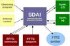 |
Fig. 3 Schematic diagram of operations made by SDAI. The communication with the observing program and antenna control (yellow boxes), as well as the FFTS (red boxes), are made through sockets. Tuning is performed by a continuous setting of the synthesizers through USB connections. Resulting spectra are written in FITS format for the subsequent analysis. |
Summary of observations.
The astronomical results reported here are the first using the whole fully assembled system. The observations were performed aimed to test:
-
the performance of the whole backend, particularly the differentIF channels;
-
the quality and stability of tunings with different synthesizers;
-
the band stability during long integrations;
-
the performances of the different filters;
-
the image sideband reflections, spurious signals, spikes, aliasing.
A summary of the observations carried out in August and September 2011 is presented in Table 5. We used the Q-band receiver attached to the DSS-54 antenna, and only the broad-band setup of the FFTS (setup 1 in Table 4), with just one FFTS card (e.g., a total instantaneous bandwidth of 1.5 GHz). A second set of observations is planned to test the high-resolution modes, which will be reported as a Q-band catalog (Rizzo et al., in prep.).
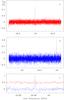 |
Fig. 4 CS J = 1 → 0 line observed toward W3(OH). a) Line frequency in the band center. b) Line frequency next to an edge of the band. c) A 40-MHz zoom of both spectra centered at the line. The comparison of both spectra is satisfactory, both in frequency and intensity scale. The upper spectrum a) is less noisy than the lower one b) owing to different integration times (8 and 3 min, respectively). |
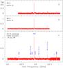 |
Fig. 5 W51D at 43 GHz. a) Spectrum obtained using the synthesizer LO. b) The same, but using the synthesizer HI. c) Combined spectrum, covering a bandwidth of 1.9 GHz. This test was made to check the consistency of both synthesizers. Line identification is included in the bottom spectrum. |
Spectra of the observations reported here were reduced with simple procedures (e.g., baseline subtraction and FFT components editing) using CLASS. No spikes were noted when the input signal level to the FFTS was within the working regime (see Table 3); however, some spikes (up to four, depending on the observing frequency) were recorded when the signal was below these levels. When possible, the spectra were compared with published data, provided in Table 5. Some of the resulting spectra, after reduction, are shown in Figs. 4–8.
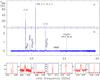 |
Fig. 6 2.6 GHz bandwidth spectrum of Orion KL. a) Full spectrum, dominated by the SiO J = 1 → 0 lines, especially the vibrationally excited states v = 1 and v = 2. b) The same, but zoomed in intensity to bring out other lines. Lower panels: detailed view of some spectral features. From left to right: SiO J = 1 → 0, v = 2; 29SiO J = 1 → 0, v = 0, probably blended to H83δ; H53α, He53α, H89ϵ, and (CH3)2CO 108,2 → 107,4; SiO J = 1 → 0, v = 1; SiO J = 1 → 0, v = 0, and a U line; H66β; the 44 GHz methanol maser. |
In Fig. 4 the CS J = 1 → 0 line toward W3(OH) is plotted. While in Fig. 4a the line is in the center of the band, it is close to a band edge in Fig. 4b. These observations were made to test the frequency and intensity stabilities in different parts of the band. As Fig. 4c shows, the comparison between both spectra are considered satisfactory.
Figure 5 shows a spectrum of the star-forming region W51D at 43 GHz. Because this frequency may be tuned using both synthesizers, we used this case for cross-checking frequencies and intensities using different synthesizers (LO and HI in Figs. 5a and b, respectively) and during different days. System temperatures were similar during the three days, and therefore the noise level differences are due to different integration times (16 and 30 min in Figs. 5a and b, respectively). The combined spectrum, 1.9 GHz width, is depicted in Fig. 5c. The spectrum is dominated by radio recombination lines (RRLs), the thermal (v = 0) SiO J = 1 → 0 line, and its corresponding masers v = 1 and v = 2.
Figure 6 displays the well-known spectral wealth of Orion KL. The combined spectrum has 2.6 GHz of bandwidth, and a total integration time of 45 min. As Fig. 6a shows, the spectrum is dominated by the thermal (v = 0) and maser (v = 1 and 2) emission of SiO J = 1 → 0. In Fig. 6b, some lower-intensity lines are noted, including the thermal isotopomer 29SiO J = 1 → 0, some RRLs, organic compounds, and the 44 GHz methanol maser. The lower panels of Fig. 6 show a zoom of these and other lines, detailed in the caption. Part of this spectrum is reported for the first time. The strong SiO maser at 43.122 GHz was used to study possible aliasing effects and to measure the image sideband rejection; no aliasing was measured, and the image band is attenuated by more than 6, 15, and 25 dB at 25, 50, and 75 MHz of the pass band borders, respectively.
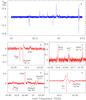 |
Fig. 7 Spectrum of Sgr B2(M). a) Full spectrum, showing the complexity of this source. b)–e) Detailed view of some spectral features, together with the corresponding identifications. |
Figure 7 depicts the spectrum toward Sgr B2(M), centered at 42.75 GHz, and having 1.5 GHz of bandwidth. A total of 24 min (on source) was employed. The full spectrum is shown in Fig. 7a, while in Figs. 7b–e a detailed zoom and line identification are displayed. As usual in this source, a mixture of emission and absorption features appear. Although no maser SiO lines are detected, the presence of the rare isotopomer 30SiO J = 1 → 0 line is remarkable, as well as several complex organic compounds and reactive ions.
A broad composite spectrum toward TMC-1 is shown in Fig. 8. The bandwidth is 8.5 GHz, and the total integration time is 39 min; each 1.5 GHz-wide individual scan was integrated for 3 to 8 min, as the different noise levels along the observed band show. More than a dozen lines are identified. In this source, the lines are detected just in a single channel, because the intrinsic linewidths are lower than 0.5 km s-1 (Takano et al. 1998), which is only a fraction of the channel width (1.2 km s-1) at Q-band frequencies.
4. Improvements and upgrades
As mentioned above, the commissioning tests reported here were made in the low-resolution mode (setup 1 in Table 4), and using just a single FFTS card. A second FFTS card and the high-resolution cores are planned for installation at the beginning of 2012. In low resolution, these new configurations will provide an instantaneous bandwidth of 3 GHz, which would be connected to a single or both polarizations, and tuned at the same or different central frequencies. Furthermore, the system will provide high-resolution spectra (see Table 4), for up to two bands of 100 or 500 MHz. Once these upgrades are completed, and the software is modified, we plan to start a second set of commissioning observations.
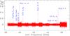 |
Fig. 8 8.5 GHz bandwidth spectrum toward TMC-1. The full spectrum is a composite of individual scans of 1.5 GHz of bandwidth. Integration time of individual scans ranges from 3 to 8 min, which is easy to note by different noise levels. Some of the identified lines are also indicated. |
As part of the normal operation and maintenance activities, RF cables and cryogenics will be checked and replaced if necessary. The incorporation of new programmable attenuators and amplifiers adapted to the frequency range of the IF processor are also planned; these devices will maintain the signal within the working limits of the FFTS (Table 3) and will improve the flatness of the instantaneous pass band. New releases of SDAI will ease the simultaneous observations of different bandwidths and resolutions.
The system performance, in particular regarding possible harmonics and image sideband rejection, will be a subject of continuous attention. Finally, the backend can be made to be even more productive by the incorporation of two other FFTS cards, which will increase the instantaneous bandwidth to up to 6 GHz. The IF processor and the SDAI software are already prepared for such an upgrade.
5. Conclusions
The facility reported here constitutes a significant enhancement to the radio astronomy capabilities at the MDSCC. The new backend performance fulfills the initial objectives. For the commissioning activities, we chose a set of sources based on line profile variety and spectral richness. The resulting spectra are considered to be of high quality. When the input signal to the FFTS fits within its working limits (Table 3), no spikes were noted and the baseline subtraction was performed without major inconveniences; ripples, when present, are easily removed by a FFT analysis. Weak RRLs are clearly distinguished from continuum after a few minutes of integration, and very narrow lines are easily recognized, although they appear in just a single channel.
This new facility improves the efficiency of the Robledo complex in two ways. On the one hand, simultaneous observations of several spectral lines in two polarizations are now possible, which makes better use of the available time, and improves the subsequent analysis by avoiding pointing and calibration problems. On the other hand, new scientific categories can now be addressed, such as spectral line surveys and extragalactic radio astronomy.
The incorporation of a second FFTS board and high-resolution cores are ongoing. First results using the high-resolution modes are planned, together with a Q-band catalog (Rizzo et al., in prep.), and possibly line surveys.
Finally, we point out that the project is in constant evolution, which means that the performance and reliability of the whole system is regularly checked and improved.
Inter-Range Instrumentation Group, format B. IRIG-B is one of the most extended standard time codes used in electronic equipment where serial times are generated for correlation of data with time. See http://www.irigb.com
CLASS is part of the GILDAS software, developed by IRAM. See http://www.iram.fr/IRAMFR/GILDAS
Acknowledgments
The backend was funded mostly through INTA grant 2009/PC0002CAB. This paper has been partially supported by MICINN
under grants AYA2006-14876 and AYA2009-07304, and by the program CONSOLIDER INGENIO 2010, under grant Molecular Astrophysics: The Herschel and ALMA Era ASTROMOL (Ref.: CSD2009-00038). Part of this research was carried out at the Jet Propulsion Laboratory, California Institute of Technology, under a contract with the National Aeronautics and Space Administration. J.R.R. wishes to thank Clemens Thum and Salvador Sánchez (IRAM Granada) for their guidance in the first stages of the project. We are also indebted to Andreas Bell and Bernd Klein (MPIfR), and Ralf Henneberger (RPG), for their kind support about the FFTS and its libraries. We acknowledge our referee, Dr. Jeff Mangum, for thoroughly reading the manuscript, and for comments and suggestions that allowed us to greatly improve this paper.
References
- Busquet, G., Palau, A., Estalella, R., et al. 2009, A&A, 506, 1183 [NASA ADS] [CrossRef] [EDP Sciences] [Google Scholar]
- Deguchi, S., Miyazaki, A., & Minh, Y. C. 2006, PASJ, 58, 979 [NASA ADS] [CrossRef] [Google Scholar]
- Goddi, C., Greenhill, L. J., Humphreys, E. M. L., et al. 2009, ApJ, 691, 1254 [NASA ADS] [CrossRef] [Google Scholar]
- Gómez, J. F., de Gregorio-Monsalvo, I., Suárez, O., & Kuiper, T. B. H. 2006, AJ, 132, 1322 [NASA ADS] [CrossRef] [Google Scholar]
- Haschick, A. D., Menten, K. M., & Baan, W. A. 1990, ApJ, 354, 556 [NASA ADS] [CrossRef] [Google Scholar]
- Horiuchi, S., García-Miró, C., Rizzo, J. R., et al. 2010, in EGU General Assembly 2010, held 2–7 May, 2010 in Vienna, Austria, 12, 13408 [Google Scholar]
- Kaifu, N., Ohishi, M., Kawaguchi, K., et al. 2004, PASJ, 56, 69 [NASA ADS] [CrossRef] [Google Scholar]
- Kawaguchi, K., Takano, S., Ohishi, M., et al. 1992, ApJ, 396, L49 [NASA ADS] [CrossRef] [Google Scholar]
- Kim, J., Cho, S.-H., Oh, C. S., & Byun, D.-Y. 2010, ApJS, 188, 209 [NASA ADS] [CrossRef] [Google Scholar]
- Klein, B., Philipp, S. D., Krämer, I., et al. 2006, A&A, 454, L29 [NASA ADS] [CrossRef] [EDP Sciences] [Google Scholar]
- Klein, B., Krämer, I., Hochgürtel, S., et al. 2008, in Ninteenth Int. Symp. Space Terahertz Technology, 192 [Google Scholar]
- Suárez, O., Gómez, J. F., & Morata, O. 2007, A&A, 467, 1085 [NASA ADS] [CrossRef] [EDP Sciences] [Google Scholar]
- Takano, S., Suzuki, H., Ohishi, M., et al. 1990, ApJ, 361, L15 [NASA ADS] [CrossRef] [Google Scholar]
- Takano, S., Masuda, A., Hirahara, Y., et al. 1998, A&A, 329, 1156 [NASA ADS] [Google Scholar]
- Turner, B. E., Zuckerman, B., Palmer, P., & Morris, M. 1973, ApJ, 186, 123 [NASA ADS] [CrossRef] [Google Scholar]
All Tables
All Figures
|
Fig. 1 Concept diagram of the signal path from the antenna receiver (HEMT) through the backend. The first stage of the backend is the IF processor, followed by the FFT spectrometer. Finally, data are processed and recorded on a dedicated PC (see text). |
| In the text | |
|
Fig. 2 Block diagram of the IF processor. Input polarizations are marked by red and green colors. The signals are divided into two channels, LO and HI, for each polarization, providing four output channels at base band. |
| In the text | |
|
Fig. 3 Schematic diagram of operations made by SDAI. The communication with the observing program and antenna control (yellow boxes), as well as the FFTS (red boxes), are made through sockets. Tuning is performed by a continuous setting of the synthesizers through USB connections. Resulting spectra are written in FITS format for the subsequent analysis. |
| In the text | |
|
Fig. 4 CS J = 1 → 0 line observed toward W3(OH). a) Line frequency in the band center. b) Line frequency next to an edge of the band. c) A 40-MHz zoom of both spectra centered at the line. The comparison of both spectra is satisfactory, both in frequency and intensity scale. The upper spectrum a) is less noisy than the lower one b) owing to different integration times (8 and 3 min, respectively). |
| In the text | |
|
Fig. 5 W51D at 43 GHz. a) Spectrum obtained using the synthesizer LO. b) The same, but using the synthesizer HI. c) Combined spectrum, covering a bandwidth of 1.9 GHz. This test was made to check the consistency of both synthesizers. Line identification is included in the bottom spectrum. |
| In the text | |
|
Fig. 6 2.6 GHz bandwidth spectrum of Orion KL. a) Full spectrum, dominated by the SiO J = 1 → 0 lines, especially the vibrationally excited states v = 1 and v = 2. b) The same, but zoomed in intensity to bring out other lines. Lower panels: detailed view of some spectral features. From left to right: SiO J = 1 → 0, v = 2; 29SiO J = 1 → 0, v = 0, probably blended to H83δ; H53α, He53α, H89ϵ, and (CH3)2CO 108,2 → 107,4; SiO J = 1 → 0, v = 1; SiO J = 1 → 0, v = 0, and a U line; H66β; the 44 GHz methanol maser. |
| In the text | |
|
Fig. 7 Spectrum of Sgr B2(M). a) Full spectrum, showing the complexity of this source. b)–e) Detailed view of some spectral features, together with the corresponding identifications. |
| In the text | |
|
Fig. 8 8.5 GHz bandwidth spectrum toward TMC-1. The full spectrum is a composite of individual scans of 1.5 GHz of bandwidth. Integration time of individual scans ranges from 3 to 8 min, which is easy to note by different noise levels. Some of the identified lines are also indicated. |
| In the text | |
Current usage metrics show cumulative count of Article Views (full-text article views including HTML views, PDF and ePub downloads, according to the available data) and Abstracts Views on Vision4Press platform.
Data correspond to usage on the plateform after 2015. The current usage metrics is available 48-96 hours after online publication and is updated daily on week days.
Initial download of the metrics may take a while.