| Issue |
A&A
Volume 542, June 2012
|
|
|---|---|---|
| Article Number | A102 | |
| Number of page(s) | 9 | |
| Section | Cosmology (including clusters of galaxies) | |
| DOI | https://doi.org/10.1051/0004-6361/201118444 | |
| Published online | 14 June 2012 | |
A cosmological view of extreme mass-ratio inspirals in nuclear star clusters
1 INAF – Osservatorio Astronomico di Padova, Vicolo dell’Osservatorio 5, 35122 Padova, Italy
e-mail: This email address is being protected from spambots. You need JavaScript enabled to view it.
2 Università Milano Bicocca, Dipartimento di Fisica G. Occhialini, Piazza delle Scienze 3, 20126 Milano, Italy
3 School of Physics and Astronomy, University of Birmingham, Edgbaston, Birmingham B15 2TT, UK
4 Centre for Astrophysics and Supercomputing, Swinburne University of Technology, Hawthorn, 3122 Victoria, Australia
5 Max-Planck Institut für Astrophysik, Karl-Schwarzschild-Strasse 1, 85748 Garching, Germany
Received: 11 November 2011
Accepted: 9 May 2012
Abstract
There is increasing evidence that many galaxies host both a nuclear star cluster (NC) and a super-massive black hole (SMBH). Their coexistence is particularly prevalent in spheroids with stellar mass 108–1010 M⊙. We study the possibility that a stellar-mass black hole (BH) hosted by a NC inspirals and merges with the central SMBH. Due to the high stellar density in NCs, extreme mass-ratio inspirals (EMRIs) of BHs onto SMBHs in NCs may be important sources of gravitational waves (GWs). We consider sensitivity curves for three different space-based GW laser interferometric mission concepts: the Laser Interferometer Space Antenna (LISA), the New Gravitational wave Observatory (NGO) and the DECi-hertz Interferometer Gravitational wave Observatory (DECIGO). We predict that, under the most optimistic assumptions, LISA and DECIGO will detect up to thousands of EMRIs in NCs per year, while NGO will observe up to tens of EMRIs per year. We explore how a number of factors may affect the predicted rates. In particular, if we assume that the mass of the SMBH scales with the square of the host spheroid mass in galaxies with NCs, rather than a linear scaling, then the event rates are more than a factor of 10 lower for both LISA and NGO, while they are almost unaffected in the case of DECIGO.
Key words: gravitational waves / black hole physics / galaxies: nuclei / galaxies: star clusters: general / cosmology: theory
© ESO, 2012
1. Introduction
Nuclear star clusters (NCs) are massive star clusters located at the centre of galaxies (see, e.g., Böker 2010, for a recent review). They are common and quite ubiquitous, as the fraction of galaxies with unambiguous NC detection is ~75 per cent in late-type (Scd-Sm) spirals (Böker et al. 2002), ~50 per cent in earlier-type (Sa-Sc) spirals (Carollo et al. 1997) and ~70 per cent in low and intermediate luminosity early-type galaxies (Graham & Guzmán 2003; Côté et al. 2006). The typical size of NCs is similar to that of Galactic globular clusters (GCs, half-light radius ≈ 2–5 pc, Geha et al. 2002; Böker et al. 2004; Côté et al. 2006), but NCs are 1–2 orders of magnitude brighter (and more massive) than Galactic GCs (Walcher et al. 2005). Unlike most of the Galactic GCs, NCs have often a complex star formation (SF) history, with multiple episodes of SF (Rossa et al. 2006; Walcher et al. 2006). NCs are of course not the Bahcall-Wolf (Bahcall & Wolf 1976, 1977) cusps predicted to exist around SMBHs: NC sizes are much larger (e.g. Merritt & Szell 2006) and they are observed in galaxies thought not to host SMBHs (e.g. Ferrarese et al. 2006).
NCs obey scaling relations with host-galaxy properties (such as galaxy mass, spheroid luminosity and velocity dispersion, e.g., Balcells et al. 2003; Graham & Guzmán 2003; Balcells et al. 2007; Ferrarese et al. 2006; Wehner & Harris 2006; Rossa et al. 2006; Graham & Driver 2007). These scaling relations are similar to those observed for super-massive black holes (SMBHs), suggesting that there is a link between NCs and SMBHs. Various studies (Ferrarese et al. 2006; Wehner & Harris 2006) indicate that SMBHs (NCs) are found predominantly above (below) a stellar mass threshold M ∗ ≈ 1010 M⊙. However, the presence of a SMBH and that of a NC do not seem to be mutually exclusive. In addition to the Milky Way (MW, see, e.g., Schödel et al. 2007, 2009), Filippenko & Ho (2003) identified at least one galaxy (NGC 4395) hosting both a SMBH and a NC, and Graham & Driver (2007) subsequently reported the existence of two additional such galaxies (NGC 3384 and NGC 7457). The sample of galaxies hosting both a SMBH and a NC was substantially increased by Gonzalez Delgado et al. (2008, 2009), Seth et al. (2008a) and Graham & Spitler (2009). In particular, Graham & Spitler (2009) identify a dozen NCs in galaxies that host SMBHs, whose mass was already determined via dynamical measurements. Furthermore, Graham & Spitler (2009) suggest that most spheroids with stellar masses ranging from 108 M⊙ to a few 1010 M⊙ might host both a SMBH and a NC.
NCs have been proposed as important sources of gravitational waves (GWs, Poincaré 1905; Einstein 1916, 1918), originating from mergers between stellar-mass black hole (BH) binaries (Miller & Lauburg 2009; see also Freitag 2003; Hopman et al. 2007; O’Leary et al. 2009; O’Shaughnessy et al. 2010). In fact, because of their relatively high escape velocity, NCs should be able to retain most of their stellar-mass BHs (Miller & Lauburg 2009), in spite of natal kicks and gravitational interactions (although the presence of a SMBH inside the NC might affect this scenario, see, e.g., Merritt 2006, 2009). Furthermore, three-body interactions are expected to be very frequent in NCs, given their high central density, leading to shrinking and coalescence of hard binaries. For these reasons, Miller & Lauburg (2009) predict that tens of BH–BH mergers per year in NCs will be observable with the advanced Laser Interferometer Gravitational-wave Observatory (advanced LIGO, Harry et al. 2010). Given the increasing evidence of the coexistence between SMBHs and NCs in some galaxies, we propose that mergers between SMBHs and stellar BHs may also occur in NCs. Such events fall within the class of extreme mass-ratio inspirals (EMRIs, see Amaro-Seoane et al. 2007, for a review) and may be detected by space-borne interferometers. At present, it is still fairly uncertain what mission could fly in the future. As reference, we consider the published sensitivity performance of the Laser Interferometer Space Antenna (LISA, Bender et al. 1998; Gair et al. 2010), the European New Gravitational wave Observatory (NGO, derived from the previous LISA proposal, Amaro-Seoane et al. 2012a,b) and the DECi-hertz Interferometer Gravitational wave Observatory (DECIGO, Kawamura et al. 2006).
In this paper, we investigate the capture rate of BHs onto SMBHs in NCs which yield EMRIs1 and we estimate their detectability by future gravitational-wave space-based observatories.
2. Method
In this section, we derive the rate of EMRIs in NCs and we infer an expected detection rate of such events by LISA, NGO and DECIGO.
2.1. The detection rate
The detection rate R of EMRIs in NCs can be expressed as (see, e.g., Miller 2002; Mapelli et al. 2010) 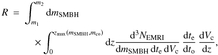 (1)where m1 and m2 are the minimum and maximum SMBH mass (mSMBH); NEMRI is the number of EMRIs of SMBH–BH binaries; te and to are the time in the rest frame of the source and of the observer, respectively (thus,
  ). Vc is the comoving volume. In flat Λ cold dark matter (ΛCDM),
 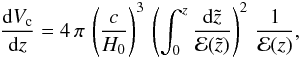 (2)where c is the light speed, H0 is the Hubble constant (H0 = 71 km s-1 Mpc-1) and
 ![Mathematical equation: \hbox{${\mathcal E}(z)=\left[\Omega_\Lambda+(1+z)^3\Omega_{\rm M}\right]^{1/2}$}](/articles/aa/full_html/2012/06/aa18444-11/aa18444-11-eq26.png) , with ΩΛ = 0.73 and ΩM = 0.27 (Larson et al. 2011).
, with ΩΛ = 0.73 and ΩM = 0.27 (Larson et al. 2011).
The quantity zmax(mSMBH,mco) is the maximum redshift at which an event can be detected with a sky-location and orientation averaged signal-to-noise ratio ⟨ SNR ⟩ ≥ 10 by a single interferometer. Thus, zmax(mSMBH,mco) defines the instrumental horizon of a given detector. In observations with a network of instruments, the signal-to-noise ratio scales as the square root of the number of instruments, and in this respect the results presented here should be considered as conservative. The maximum redshift depends on (i) the mass of the SMBH mSMBH, (ii) the mass of the companion (mco) that merges with the SMBH, (iii) the orbital eccentricity e(t), (iv) the spin parameter of the SMBH ( , where S is the modulus of the angular momentum of the SMBH, c is the speed of light and G is the gravitational constant), and on various other parameters, as well as on the sensitivity of the instrument. In this paper, we adopt mco = 10 M⊙, corresponding to the typical mass of a stellar-mass BH. We consider different values of the eccentricity and of the spin parameter. See Appendix A for details on the derivation of zmax(mSMBH,mco).
The EMRI rate per unit mass, time and volume can be written as: 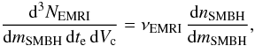 (3)where nSMBH is the comoving density of SMBHs surrounded by NCs and νEMRI is the rate of EMRIs (i.e., the rate of mergers that end-up as EMRIs) per SMBH.
Graham & Spitler (2009) indicate that SMBHs coexist with NCs in spheroids with mass 108 ≤ msph/M⊙ ≤ 1010. The questions (i) whether there is a scaling between the mass of the SMBH and that of the host spheroid, and (ii) whether such relation is valid for all SMBH masses have been debated for a long time. Marconi & Hunt (2003, hereafter MH03) find that mSMBH ~ 0.002 msph, but there might be large deviations (up to a factor of 10) from this value for low-mass ( ≤ 106 M⊙) SMBHs (see, e.g., Table 2 of Graham & Spitler 2009). Graham (2012a, hereafter G12a) and Graham (2012b, hereafter G12b) propose that the mass of the SMBH scales (nearly) with the square of the host spheroid mass in galaxies with NCs (i.e. galaxies with msph < 1011 M⊙), while it scales linearly with the host spheroid mass in high-mass galaxies (which often have partially depleted cores). In particular, G12a proposes that log 10(mSMBH/M⊙) = (8.38 ± 0.17) + (1.92 ± 0.38) log 10(msph/7 × 1010 M⊙) for galaxies with NCs. The BH mass range corresponding to 108 ≤ msph/M⊙ ≤ 1010 is 2 × 10⁵–2 × 10⁷ M⊙ and 8 × 10²–5.7 × 10⁶ M⊙, according to the results by MH03 and by G12a, respectively. In the following, we will consider both cases. In particular, we define fBH(msph) = 0.002 msph and  , when adopting the formalism by MH03 and by G12a, respectively. Therefore, Eq. (1) can be rewritten as
 ![Mathematical equation: \begin{eqnarray} \label{eq:sph} R&=&4\,\pi\,\left(\frac{c}{H_0}\right)^3\int_{m_{\rm sph1}}^{m_{\rm sph2}}\,{\rm d}m_{\rm sph}\,\nu_{\rm EMRI}\nonumber\\ &&\quad\times\int_0^{z_{\rm max}[f_{\rm BH}(m_{\rm sph}), m_{\rm co}]}{\rm d}z\,f_{\rm bb}\,\frac{{\rm d}n_{\rm sph}}{{\rm d}m_{\rm sph}} \nonumber\\ &&\quad\times\,\frac{1}{(1+z)\,{\mathcal E}(z)}\,\left(\int_0^z \frac{{\rm d}\tilde{z}}{{\mathcal E}(\tilde{z})}\right)^2, \end{eqnarray}](/articles/aa/full_html/2012/06/aa18444-11/aa18444-11-eq53.png) (4)where msph1 = 108 M⊙ and msph2 = 1010 M⊙ are the minimum and the maximum mass of spheroids that host SMBHs together with NCs, respectively; fbb is the fraction of spheroids in the considered mass range (108 ≤ msph/M⊙ ≤ 1010) that host both a SMBH and a NC (we assume fbb = 1, according to Graham & Spitler 2009); nsph is the comoving density of spheroids. In Eq. (4), we used the fact that
(4)where msph1 = 108 M⊙ and msph2 = 1010 M⊙ are the minimum and the maximum mass of spheroids that host SMBHs together with NCs, respectively; fbb is the fraction of spheroids in the considered mass range (108 ≤ msph/M⊙ ≤ 1010) that host both a SMBH and a NC (we assume fbb = 1, according to Graham & Spitler 2009); nsph is the comoving density of spheroids. In Eq. (4), we used the fact that 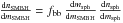 .
.
We can derive nsph from the comoving density of halos nh, assuming that spheroids with mass msph are located in halos with total mass mh = msph/p. Thus, Eq. (4) can be rewritten as ![Mathematical equation: \begin{eqnarray} \label{eq:halo} R&=&4\,\pi\,\left(\frac{c}{H_0}\right)^3\int_{m_{\rm h1}}^{m_{\rm h2}}\,{\rm d}m_{\rm h}\,\nu_{\rm EMRI}\nonumber\\ &&\quad\times\int_0^{z_{\rm max}[f_{\rm BH}(p\,m_{\rm h}), m_{\rm co}]}{\rm d}z\,\,f_{\rm bb}\,\frac{{\rm d}n_{\rm h}}{{\rm d}m_{\rm h}} \nonumber\\ &&\quad\times\frac{1}{(1+z)\,{\mathcal E}(z)}\,\left(\int_0^z \frac{{\rm d}\tilde{z}}{{\mathcal E}(\tilde{z})}\right)^2, \end{eqnarray}](/articles/aa/full_html/2012/06/aa18444-11/aa18444-11-eq63.png) (5)where
(5)where  is the Press-Schechter function (Press & Schechter 1974; Eisenstein & Hu 1998, 1999), mh1 = msph1/p and mh2 = msph2/p. We use p = 1.06 × 10⁻² as a fiducial value, but we consider also p = 5.04 × 10⁻² and = 2.81 × 10⁻³ as upper and lower values, respectively, depending on the baryonic fraction in dark matter halos (see Appendix B for the derivation of p). In Eq. (5), we write fbb inside both integrals (in mass and redshift), although, in the following, we will assume for simplicity that fbb is a constant.
2.2. The EMRI rate
The EMRI rate νEMRI (i.e. the rate of mergers that end-up as EMRIs) is likely the most difficult quantity to estimate in Eq. (5), as it depends on the dynamics and on the relativistic effects in the neighborhoods ( ≲ 10-2 pc) of the SMBH. In particular, the collisional dynamics of relativistic star clusters around SMBHs is poorly understood. The presence of the SMBH potential well strongly affects the inner regions of the star cluster and the dynamics of binary stars (Alexander 1999, 2003, 2005; Alexander & Hopman 2009; Hopman 2009). To derive νEMRI in an accurate way is beyond the aims of this paper. Here, we will adopt approximate rates derived by Merritt et al. (2011). Capture of stars on EMRI orbits can be driven by resonant relaxation (Rauch & Tremaine 1996; Hopman & Alexander 2006a), by two-body relaxation (Merritt et al. 2011) or even by dynamical friction (Antonini & Merritt 2012), that is by physical processes where background stars exert torques on the stellar orbits. The capture of a star is hampered by the so-called Schwarzschild barrier (Merritt et al. 2011), that is by an angular-momentum barrier associated with the value of the orbital angular momentum at which the background torques become ineffective due to the Schwarzschild precession of the orbit2. Merritt et al. (2011) analyze various mechanisms to penetrate the Schwarzschild barrier (based on classical non-resonant relaxation), and derive a time scale tloss for stars to “definitely” cross the barrier (see their Eq. (71) and Tables 2, 3).
According to the results by Merritt et al. (2011), we approximate νEMRI as:  (6)where
  is the number of stars initially with semi-major axis (with respect to the SMBH) a ~ 2–10 × 10-3 pc. is basically unknown. We also note that the adopted value of tloss was derived for a SMBH-to-BH mass ratio equal to 2 × 10⁴. Therefore it is suited for mSMBH = 2 × 10⁵ M⊙ (adopting mco = 10 M⊙). On the other hand, most of the contribution for the detection rates (in Table 1) comes from such “low-mass” SMBHs, as we will discuss in the next section.
We stress that, at the moment of capture, the eccentricity is likely very high (e.g., Merritt et al. 2011, and references therein; but see Miller et al. 2005, for the effect of tidal disruption of binaries), and GWs are emitted in short pulses during pericentre passages. Then, the orbit gradually shrinks and circularizes (over a timescale of ~ 103–108 yr, e.g. Barack & Cutler 2004b), because of GW emission, and the GW emission can be observed as continuous. In the next section, we define eLSO as the eccentricity at the last stable orbit (LSO) and we integrate it back in time accounting for GW circularization (see Appendix A and Barack & Cutler 2004a).
We note also that Merritt et al. (2011) adopt a steady-state, cuspy model of the galactic centre (e.g., Sigurdsson & Rees 1997; Hopman & Alexander 2006b; Freitag et al. 2006), to derive the estimate that we use in Eq. (6). In these models, which are relaxed and strongly mass segregated, the mass within ~0.1 pc of the SMBH is contributed mainly by stellar-mass BHs. Therefore, two-body scatterings dominate the orbital evolution in proximity of the Schwarzschild barrier (e.g., Freitag et al. 2008; Alexander & Hopman 2009), whereas dynamical friction is negligible.
If stars in the central parsec of a galaxy follow a flat core rather than a relaxed cusp, the time for a stellar-mass BH (initially located out of the core) to reach the centre of the host galaxy can easily exceed the Hubble time (Merritt 2010). Thus, in flat cores, the number of stellar BHs within the influence radius of the SMBH is still low with respect to the total number of objects, including lower-mass remnants and stars. In this case, dynamical friction can be more important than two-body scatterings to penetrate the Schwarzschild barrier (according to the new, more general expression of dynamical friction, derived by Antonini & Merritt 2012). This likely leads to lower EMRI rates in the case of flat cores and deserves further studies.
Whether the galaxies hosting a NC have a central stellar density cusp or a flat core is an open question. The MW, which was long believed to have a steeply-rising mass density near the SMBH, was recently found to have a parsec-scale core in the old red giant branch (RGB) stellar component (Buchholz et al. 2009; Do et al. 2009; Bartko et al. 2010). Other MW-like galaxies, hosting both a NC and a SMBH at their centre, might behave in the same way. Therefore, steady-state mass segregated models might be inappropriate to describe a MW-like galactic centre. On the other hand, only the RGB stars were observed to follow a flat core distribution in the central parsec of the MW, while the non-relaxed young stars show a rather cuspy profile (e.g., Do et al. 2009). We do not know whether the old main-sequence stars and especially the stellar remnants follow the same cored distribution as RGB stars (e.g., Dale et al. 2009; Davies et al. 2011).
A further possible caveat is that a currently cored profile might have been cuspy in the past, and then the cusp was destroyed as a consequence of dynamical effects (e.g., Merritt 2010; Yusef-Zadeh et al. 2012). At the moment, the most likely scenario to explain the removal of the cusp and its transformation into a core is that of binary scouring as a consequence of a galaxy merger (Gualandris & Merritt 2012). In this case, the central cusp of stellar BHs reforms in a time that is at least one relaxation time, and the number of BHs in the proximity of the SMBH is smaller than in relaxed multi-mass models.
In summary, whether galaxies hosting NCs have a central stellar cusp or a core, and for how long these profiles survive are very uncertain issues. Our predictions for the detectable EMRI rate, based on a mass-segregated cuspy model, represent the most optimistic case and should be regarded as upper limits.
3. Results
3.1. Maximum redshift
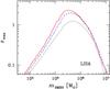 |
Fig. 1 zmax in the case of LISA, as a function of mSMBH for three different simulations. In all the shown models, j = 1 and Tmission = t0 = 5 yr (see Table 1). Solid line (red on the web): model with eLSO = 0.3. Dashed line (blue on the web): model with eLSO = 0.5. Dotted black line: model with eLSO = 0.7. |
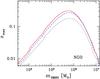 |
Fig. 2 zmax in the case of NGO, as a function of mSMBH for three different simulations. In all the shown models, j = 1 and Tmission = t0 = 5 yr (see Table 2). Solid line (red on the web): model with eLSO = 0.3. Dashed line (blue on the web): model with eLSO = 0.5. Dotted black line: model with eLSO = 0.7. |
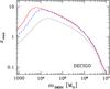 |
Fig. 3 zmax in the case of DECIGO, as a function of mSMBH for three different simulations. In all the shown models, j = 1 and Tmission = t0 = 5 yr (see Table 3). Solid line (red on the web): model with eLSO = 0.3. Dashed line (blue on the web): model with eLSO = 0.5. Dotted black line: model with eLSO = 0.7. |
Figures 1–3 show the maximum redshift (zmax) as a function of mSMBH in the case of LISA, NGO and DECIGO, respectively. In these figures, t0 = 5 yr and Tmission = 5 yr. Here, the value t0 is the assumed time before the plunge-in, i.e. the time elapsed between the beginning of the observation with the gravitational interferometer and the moment in which the companion reaches the LSO (in this paper, we study the cases where t0 = 5, 6, 10 and 15 yr). Tmission is defined as the duration of the mission. In this paper, we consider Tmission = 5 and 2 yr as two fiducial values of the mission duration, for the three considered gravitational experiments (see, e.g., Gair et al. 2010). We remind that zmax was obtained for a sky-location and orientation averaged signal-to-noise ratio higher than 10 (see Sect. 2.1 and Appendix A).
In the case of LISA (Fig. 1), zmax reaches high values (z ~ 2) for mSMBH ~ 105–106 M⊙ and eccentricity at the LSO eLSO ≤ 0.5. The value of zmax for LISA drops below ~1 for mSMBH < 105 M⊙ and for mSMBH > 2 × 10⁶ M⊙. The behaviour of zmax for NGO (Fig. 2) is similar to that of LISA, in the sense that zmax drops quite fast for mSMBH < 105 M⊙ and for mSMBH > 2 × 10⁶ M⊙. On the other hand, the maximum value of zmax for NGO (obtained for mSMBH ~ 105–106 M⊙) is zmax ~ 0.3, much lower than in the case of LISA.
In the case of DECIGO (Fig. 3), zmax ~ 3 for mSMBH ~ 105 M⊙, but zmax keeps rising for smaller BH masses and reaches a value of 8 − 10 for mSMBH ~ 5 × 10³ M⊙. We stress that the existence of BHs in the 103 − 105 M⊙ mass range is still controversial (e.g., Miller & Colbert 2004, and references therein).
Simulated values of the rate R for the old LISA configuration.
3.2. Detection rates
Tables 1–3 summarize the estimated values of the detection rate R for the simulated models, in the case of LISA, NGO and DECIGO, respectively.
Figure 4 shows the behaviour of R as a function of eLSO in the case of LISA, NGO and DECIGO. In the top panel of Fig. 4, the mSMBH − msph relation follows the prescriptions by G12a, while in the bottom panel it follows the linear scaling derived by MH03. Tables 1–3 and Fig. 4 indicate that LISA and DECIGO are expected to detect a factor of ≳ 100 more EMRI events than NGO.
A comparison among Tables 1–3 indicates that LISA, NGO and DECIGO have similar responses to the physical parameters influencing EMRI events (although the overall sensitivity of NGO is much lower than that of the other two instruments). In particular, for all the considered space-borne instruments, R is slightly affected by the spin parameter. R mildly depends on the eccentricity (Fig. 4): values of eLSO ≥ 0.7 often correspond to lower values of R, since zmax is lower for eLSO ≥ 0.7.
Tables 1–3 show that the detection rate is very sensitive to the parameter t0, which indicates how far the observed systems are from final coalescence. R rapidly decreases as t0 increases. To accurately derive R, we should “average” our results over a distribution of values of t0. This is beyond the aims of this paper. Therefore, we will consider the estimates of R obtained for t0 = 5 yr as upper limits, as assuming t0 = 5 yr maximizes the probability of observing a merger event for all the duration of the mission. Furthermore, the detection rate sensibly depends on the duration of the mission (Tmission). If we assume that LISA, NGO and DECIGO will operate only for two years and that t0 = 5 yr, the expected rates are lower by a factor of ≈ 10.
In our approximate model, R scales linearly with νEMRI: this quantity is highly uncertain, but our estimates can be rescaled for different choices of νEMRI (the adopted values can be considered as upper limits). Finally, the halo-to-spheroid mass ratio (p) changes dramatically the rate R, and is another poorly constrained factor.
From Fig. 4 and from Tables 1–3, we note also that there is a strong dependence of R on the assumed model for fBH(msph), that is on the assumed mSMBH − msph relation. In the case of both LISA and NGO, the relation derived by G12a predicts a factor of ≈ 10 less detections than the linear scaling obtained by MH03. This is not true for DECIGO, whose expected detection rate is almost unaffected by the assumed fBH(msph).
The reason of this behaviour is quite intuitive: the mSMBH − msph scaling relation obtained by G12a ( ) implies that relatively low mass BHs (<105 M⊙) are associated with most of the spheroids in the 108–1010 M⊙ mass range, whereas the linear scaling relation derived by MH03 predicts that SMBHs with 2 × 10⁵ M⊙ ≤ mSMBH ≤ 2 × 10⁷ M⊙ are hosted by spheroids in the same mass range as above. LISA and NGO have very low sensitivity to EMRIs with mSMBH < 105 M⊙ (Figs. 1 and 2), and this explains the low values of R when the relation by G12a is assumed. Instead, DECIGO is particularly suitable to observe EMRIs involving 104 M⊙ BHs (Fig. 3), while performing as well as LISA for mSMBH ~ 105–106 M⊙. This explains why the predicted detection rate for DECIGO is almost unaffected by the adopted mSMBH − msph scaling relation.
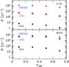 |
Fig. 4 The total detection rate R versus the adopted eccentricity at the LSO (eLSO), in the case of LISA (filled circles, red on the web), DECIGO (filled triangles, blue on the web) and NGO (filled squares). For each case, j = 1, t0 = 5 yr, Tmission = 5 yr (see Tables 1–3), p = 1.06 × 10⁻², |
Figure 5 shows the cumulative redshift distribution of the expected detections per year, that is it shows how many detections per year are expected for EMRIs at redshift < z, as a function of z. Figure 5 confirms that NGO is blind for EMRIs with z > 0.3 (as a consequence of the behaviour of zmax, see Fig. 2). From Fig. 5 we note also the very different behaviour of LISA and DECIGO with respect to the adopted mSMBH − msph scaling relation. When the MH03 relation is assumed, LISA and DECIGO have almost the same behaviour, in terms of both total detection rate and dependence on redshift: most of detectable EMRIs occur at  . Instead, when the G12a relation is assumed, most of detectable EMRIs occur at z ≲ 2 and
  for LISA and DECIGO, respectively. We stress that our predictions based on the Press-Schechter formalism might overlook many important processes affecting BH and galaxy evolution at z ≫ 1.
3.3. Comparison with previous studies
In this section, we compare the rates derived for the original LISA configuration and for NGO with those found in previous studies (e.g., Gair et al. 2004; Rubbo et al. 2006; Gair et al. 2010; Amaro-Seoane et al. 2012a). In particular, we will focus on Gair et al. (2004) and on Amaro-Seoane et al. (2012a), for LISA and NGO, respectively.
Gair et al. (2004) find a EMRI detection rate ~30–350 yr-1 (for a 10 M⊙ BH), depending on the assumed properties of the LISA mission. This result is quite consistent with our predictions, when we assume the G12a model, and is a factor of ~10 lower than our results, when we adopt the MH03 prescriptions. On the other hand, there are significant differences between our method and that by Gair et al. (2004).
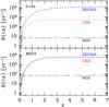 |
Fig. 5 Cumulative redshift distribution of the expected detections per year, in the case of LISA (dotted line, red on the web), DECIGO (dashed line, blue on the web) and NGO (solid line). For each case, j = 1, eLSO = 0.1, t0 = 5 yr, Tmission = 5 yr (see Tables 1–3), p = 1.06 × 10⁻², |
Firstly, Gair et al. (2004) assume a EMRI rate νEMRI ~ 10-6(mSMBH/3 × 106)3/8 yr-1 per SMBH (for mergers with a 10 M⊙ BH). This is a factor of 10 higher than our assumed EMRI rate (see Eq. (6)), when we adopt  (as in our Figs. 4 and 5).
Secondly, Gair et al. (2004) assume a different mass function for the SMBHs with respect to us. In particular, Gair et al. (2004) estimate  from the mSMBH − σ relation (where σ is the velocity dispersion, e.g., Ferrarese & Merritt 2000; Gebhardt et al. 2000; Graham et al. 2011) and from the luminosity versus σ relation (Aller & Richstone 2002). Instead, we use the mSMBH − msph relation (e.g., G12a) and the Press-Schechter formalism (Press & Schechter 1974). Furthermore, we consider only those SMBHs that can coexist with a NC (otherwise the capture rate would likely be much lower), whereas Gair et al. (2004) take into account all the BHs in the mass range 105–5 × 10⁶ M⊙, excluding only those that are located in Sc and Sd galaxies.
These differences are important, in terms of EMRI rates, as it can be shown by calculating the expected merger rate per unit volume at redshift z = 0 ( , where nSMBH(z = 0) is the number density of SMBHs at z = 0 for the considered mass range and νEMRI is the EMRI rate per SMBH). In our model, considering only SMBHs with 105 ≤ mSMBH ≤ 5 × 10⁶ M⊙ (i.e., the mass range adopted by Gair et al. 2004),
  Gpc-3 yr-1 and
  Gpc-3 yr-1, assuming the MH03 and the G12a scaling relation, respectively.
Our estimate of  derived from the G12a scaling relation is similar to the one reported in Table 2 of Gair et al. (2004), while it is one order of magnitude higher than the one reported by Gair et al. (2004) when the MH03 scaling relation is adopted instead. Our estimate of based on G12a, although very similar to the one derived by Gair et al. (2004), comes from the product between our merger rate νEMRI, which is a factor of 10 lower than the one adopted by Gair et al. (2004), and the number density of SMBHs with 105 ≤ mSMBH ≤ 5 × 10⁶ M⊙, which is a factor of 10 higher than the one in Gair et al. (2004). We stress that our value of is an upper limit, as νEMRI was obtained assuming a cuspy density profile inside the SMBH influence radius (see the discussion in Sect. 2.2) and we impose that fbb = 1, i.e. that all NCs in the considered mass range host a SMBH.
In addition, Gair et al. (2004) do not make a fully consistent cosmological integration in a ΛCDM Universe. Furthermore, the number of detectable events reported in Table 3 of Gair et al. (2004) was derived imposing that zmax cannot be higher than one. On the other hand, Gair et al. (2004) use the same kludge waveforms we adopt (from Barack & Cutler 2004a) and include an accurate treatment for detection statistics (while we consider an averaged signal-to-noise ratio over the duration of the mission). To check the importance of the redshift integration, we can substitute our Eq. (5) with a less accurate calculation (see Appendix C of Mapelli et al. 2010):  (7)where nSMBH(z = 0) is the density of SMBHs surrounded by NCs at redshift z = 0 in the 105–5 × 10⁶ M⊙ range, νEMRI is defined in Sect. 2.2, and Vc(zcut) is the comoving volume up to redshift zcut. For comparison with Gair et al. (2004), we assume that zcut is equal to the minimum between 1 and zmax. From Eq. (7), we obtain an approximate EMRI detection rate R ≈ 2 × 10³ yr-1 and R ≈ 2 × 10² yr-1, for the MH03 and the G12a scaling relation, respectively. These values are of the same order of magnitude as those listed in our Table 1, indicating that the accurate redshift integration does not affect significantly the rate in the case of LISA.
We now consider the predictions for NGO, by comparing our results with those from Amaro-Seoane et al. (2012a). In their Fig. 21, Amaro-Seoane et al. (2012a) show zmax as a function of the SMBH mass, for EMRIs with a 10 M⊙ BH. Our Fig. 2 is in fair agreement with the sky-averaged horizons shown in Fig. 21 of Amaro-Seoane et al. (2012a), taking into account that Amaro-Seoane et al. (2012a) sky-averaged horizons were calculated for Teukolsky waveform models (Teukolsky 1973), Tmission = 2 yr, random generated plunge times 0 ≤ t0/yr ≤ 5 and ⟨ SNR ⟩ ≥ 20, whereas in our Fig. 2 we adopt Barack & Cutler (2004a) waveforms, Tmission = t0 = 5 yr and ⟨ SNR ⟩ ≥ 10. The expected EMRI detection rates for NGO, that can be derived from Table 2 of Amaro-Seoane et al. (2012a) (R ≈ 15–25 yr-1) are consistent with the values reported in our Table 2, but quite optimistic for a 2-yr mission.
4. Conclusions
NCs seem to be common in galaxies, independently of the Hubble type. Recent studies (Seth et al. 2008a,b; Gonzalez Delgado et al. 2008, 2009; Graham & Spitler 2009) indicate that NCs co-exist with SMBHs in the same nucleus. The fraction of galaxies hosting both a NC and a SMBH is particularly high among spheroids with stellar mass ranging from ~108 M⊙ up to a few ~1010 M⊙. Given their high stellar densities and high escape velocities, NCs are expected to retain a large fraction of their stellar-mass BHs. Thus, it is reasonable to expect that the rate of EMRIs is enhanced in NCs.
We consider sensitivity curves for three different space-based GW laser interferometric mission concepts: the Laser Interferometer Space Antenna (LISA), the New Gravitational wave Observatory (NGO) and the DECi-hertz Interferometer Gravitational wave Observatory (DECIGO).
We show that GW signal from SMBH − BH mergers can be observed as far as redshift z ~ 2 and z ~ 8, for LISA and DECIGO, respectively, while this limit is substantially lower (z ~ 0.3) for NGO. We predict that, under the most optimistic assumptions, LISA and DECIGO will detect up to thousands of EMRIs in NCs per year, while NGO will observe up to tens of EMRIs per year.
The estimate of the detection rate R for SMBH − BH EMRIs is subject to a plethora of severe uncertainties. First, the EMRI rate depends on the dynamics and on the relativistic effects in the neighborhoods ( ≲ 10-2 pc) of the SMBH. In particular, the collisional dynamics of relativistic star clusters around SMBHs is poorly understood. Our predicted rates are upper limits, in the sense that the EMRI rate was derived assuming a mass-segregated cusp in the proximity of the SMBH (Merritt et al. 2011). The existence of a flat core rather than a mass-segregated cusp in the central parsec of galaxies can severely affect the EMRI rate (e.g., Antonini & Merritt 2012).
Furthermore, the cosmological rate of EMRIs depends on the dark-to-luminous mass ratio in galaxies, which is highly uncertain. In addition, we assumed that the fraction of spheroids that host both a SMBH and a NC is fbb = 1 for a spheroid mass range 108 ≤ msph/M⊙ ≤ 1010. This is consistent with recent observations (Graham & Spitler 2009), but is still based on a small sample of galaxies (~20–30 galaxies are known to host both a SMBH and a NC in their nucleus). If the available sample suffers from any biases, the actual fbb may be < 1, although values of fbb ≪ 1/2 are unlikely. In addition, fbb might change with redshift. In general, we do not know how NCs and SMBHs evolve with redshift and we can only assume that the halo occupation of NCs and SMBHs is the same up to z ~ 2.
The mass distribution of SMBHs is poorly understood, especially in low-mass galaxies. Previous studies (e.g., Gair et al. 2004; Amaro-Seoane et al. 2012a) derive the SMBH mass distribution from the mSMBH − σ relation, whereas we use the mSMBH − msph relation. Both relations are still largely uncertain at the low-mass tail. In the case of the mSMBH − msph relation, while previous studies proposed a linear scaling (e.g., MH03; Häring & Rix 2004), more recent data indicate a steeper scaling (, G12a, G12b). This difference implies large discrepancies (by a factor of 10) in the expected GW detection rate.
Finally, the sensitivity curves of space-borne interferometers will likely be modified in the next few years, as DECIGO is still in the design phase, while the LISA mission concept was recently abandoned and the NGO mission concept was not selected by the European Space Agency (ESA). Differences in the sensitivity curves might strongly affect the predictions that we have computed here.
Therefore, to give an accurate estimate of the detection rate R of EMRIs in NCs is beyond the scope of this paper. On the other hand, our results in Tables 1–3 and in Figs. 4 and 5 can be considered as upper limits, and indicate that EMRIs in NCs might be detected by space-born detectors. In summary, the co-existence of SMBHs and NCs can boost significantly our chance of observing GWs from EMRIs in the galactic centres, although more studies of the dynamics of relativistic star clusters are needed, to quantify this with accuracy.
In the following, we will use the definition of EMRIs as merger events occurring from an orbit with semi-major axis, at the moment of capture by the SMBH (the capture radius is defined as 8 rg, rg being the event horizon of the SMBH), less than 10-5 pc (Merritt et al. 2011).
Background torques are effective only on a timescale shorter than the fastest mechanism that changes the relative orientation of a star with respect to the gravitational field of the background stars. It can be shown that, for high eccentricity, Schwarzschild precession is the fastest mechanism (Merritt et al. 2011).
Acknowledgments
We thank the anonymous referee for the accurate and incisive comments, which helped us improving the manuscript. We thank D. Merritt for his helpful comments, M. Colpi and A. Klein for stimulating discussions. We thank Wayne Hu for making his transfer function code publicly available. A. W. Graham was supported under the Australian Research Council’s Discovery Projects funding scheme (DP110103509).
References
- Alexander, T. 1999, ApJ, 527, 835 [NASA ADS] [CrossRef] [Google Scholar]
- Alexander, T. 2003, in The Galactic black hole, Lectures on general relativity and astrophysics, ed. H. Falcke, & F. W. Hehl (Bristol: IoP, Institute of Physics Publishing), 246 [Google Scholar]
- Alexander, T. 2005, Phys. Rep., 419, 65 [NASA ADS] [CrossRef] [Google Scholar]
- Alexander, T., & Hopman, C. 2009, ApJ, 697, 1861 [NASA ADS] [CrossRef] [Google Scholar]
- Aller, M. C., & Richstone, D. 2002, AJ, 124, 3035 [NASA ADS] [CrossRef] [Google Scholar]
- Amaro-Seoane, P., Gair, J. R., Freitag, M., et al. 2007, Class. Quant. Grav., 24, 113 [Google Scholar]
- Amaro-Seoane, P., Aoudia, S., Babak, S., et al. 2012a, GW Notes, submitted [arXiv:1201.3621] [Google Scholar]
- Amaro-Seoane, P., Aoudia, S., Babak, S., et al. 2012b [arXiv:1202.0839] [Google Scholar]
- Antonini, F., & Merritt, D. 2012, ApJ, 745, 83 [NASA ADS] [CrossRef] [Google Scholar]
- Bahcall, J. N., & Wolf, R. A. 1976, ApJ, 209, 214 [NASA ADS] [CrossRef] [Google Scholar]
- Bahcall, J. N., & Wolf, R. A. 1977, ApJ, 216, 883 [NASA ADS] [CrossRef] [Google Scholar]
- Balcells, M., Graham, A. W., Domínguez-Palmero, L., & Peletier, R. F. 2003, ApJ, 582, L79 [NASA ADS] [CrossRef] [Google Scholar]
- Balcells, M., Graham, A. W., & Peletier, R. F. 2007, ApJ, 665, 1104 [NASA ADS] [CrossRef] [Google Scholar]
- Barack, L., & Cutler, C. 2004a, Phys. Rev. D, 69, 082005 [NASA ADS] [CrossRef] [Google Scholar]
- Barack, L., & Cutler, C. 2004b, Phys. Rev. D, 70, 122002 [NASA ADS] [CrossRef] [Google Scholar]
- Bartko, H., Martins, F., Trippe, S., et al. 2010, ApJ, 708, 834 [NASA ADS] [CrossRef] [Google Scholar]
- Bender, P. L., & Hils, D. 1997, Class. Quant. Grav., 14, 1439 [Google Scholar]
- Bender, P., et al. 1998, LISA Pre-Phase A Report, 2nd edn. (Garching: MPQ), MPQ, 233 [Google Scholar]
- Böker, T. 2010, Star clusters: basic galactic building blocks throughout time and space, Proc. Intern. Astron. Union, IAU Symp., 266, 58 [NASA ADS] [Google Scholar]
- Böker, T., Laine, S., van der Marel, R. P., et al. 2002, AJ, 123, 1389 [NASA ADS] [CrossRef] [Google Scholar]
- Böker, T., Sarzi, M., McLaughlin, D. E., et al. 2004, AJ, 127, 105 [NASA ADS] [CrossRef] [Google Scholar]
- Buchholz, R. M., Schödel, R., & Eckart 2009, A&A, 499, 483 [NASA ADS] [CrossRef] [EDP Sciences] [Google Scholar]
- Carollo, C. M., Stiavelli, M., de Zeeuw, P. T., & Mack, J. 1997, AJ, 114, 2366 [NASA ADS] [CrossRef] [Google Scholar]
- Côté, P., Piatek, S., Ferrarese, L., et al. 2006, ApJS, 165, 57 [NASA ADS] [CrossRef] [MathSciNet] [Google Scholar]
- Cornish, N. J. 2003 [arXiv:gr-qc/0304020] [Google Scholar]
- Cutler, C., Finn, L. S., Poisson, E., & Sussman, G. J. 1993, Phys. Rev. D, 47, 1511 [NASA ADS] [CrossRef] [Google Scholar]
- Cutler, C., Kennefick, D., & Poisson, E. 1994, Phys. Rev. D, 50, 3816 [NASA ADS] [CrossRef] [Google Scholar]
- Dale, J. E., Davies, M. B., Church, R. P., & Freitag, M. 2009, MNRAS, 393, 1016 [NASA ADS] [CrossRef] [Google Scholar]
- Davies, M. B., Church, R. P., Malmberg, D., et al. 2011, in The Galactic Center: a Window to the Nuclear Environment of Disk Galaxies, ed. M. R. Morris, Q. D. Wang, & F. Yuan (San Francisco: ASP), 212 [Google Scholar]
- Do, T., Ghez, A. M., Morris, M. R., et al. 2009, ApJ, 703, 1323 [NASA ADS] [CrossRef] [Google Scholar]
- Driver, S. P., Popescu, C. C., Tuffs, R. J., et al. 2007, MNRAS, 379, 1022 [NASA ADS] [CrossRef] [Google Scholar]
- Einstein, A. 1916, Preuss. Akad. Wiss. Berlin, Sitzungsber, Näherungsweise integration der feldgleichungen der gravitation, 688 [Google Scholar]
- Einstein, A. 1918, Preuss. Akad. Wiss. Berlin, Sitzungsber., 154 [Google Scholar]
- Eisenstein, D. J., & Hu, W. 1998, ApJ, 496, 605 [NASA ADS] [CrossRef] [Google Scholar]
- Eisenstein, D. J., & Hu, W. 1999, ApJ, 511, 5 [NASA ADS] [CrossRef] [Google Scholar]
- Farmer, A. J., & Phinney, E. S. 2003, MNRAS, 346, 1197 [NASA ADS] [CrossRef] [MathSciNet] [Google Scholar]
- Ferrarese, L., & Merritt, D. 2000, ApJ, 539, L9 [NASA ADS] [CrossRef] [Google Scholar]
- Ferrarese, L., Côté, P., Dalla Bontà, E., et al. 2006, ApJ, 644, L21 [NASA ADS] [CrossRef] [Google Scholar]
- Filippenko, A. V., & Ho, L. C. 2003, ApJ, 588, L13 [NASA ADS] [CrossRef] [Google Scholar]
- Finn, L. S., & Thorne, K. S. 2000, Phys. Rev. D, 62, 124021 [NASA ADS] [CrossRef] [Google Scholar]
- Freitag, M. 2003, ApJ, 583, L21 [NASA ADS] [CrossRef] [Google Scholar]
- Freitag, M., Amaro-Seoane, P., & Kalogera, V. 2006, ApJ, 649, 91 [NASA ADS] [CrossRef] [Google Scholar]
- Freitag, M., Dale, J. E., Church, R. P., & Davies, M. B. 2008, Formation and Evolution of Galaxy Bulges, Proceedings of the International Astronomical Union, IAU Symp., 245, 211 [NASA ADS] [Google Scholar]
- Gair, J. R., Barack, L., Creighton, T., et al. 2004, Class. Quant. Grav., 21, 1595 [NASA ADS] [CrossRef] [Google Scholar]
- Gair, J. R., Tang, C., & Volonteri, M. 2010, Phys. Rev. D, 81, 104014 [NASA ADS] [CrossRef] [Google Scholar]
- Gebhardt, K., Bender, R., Bower, G., et al. 2000, ApJ, 539, L13 [NASA ADS] [CrossRef] [Google Scholar]
- Geha, M., Guhathakurta, P., & van der Marel, R. P. 2002, AJ, 124, 3073 [NASA ADS] [CrossRef] [Google Scholar]
- González Delgado, R. M., Pérez, E., Cid Fernandes, R., & Schmitt, H. 2008, AJ, 135, 747 [NASA ADS] [CrossRef] [Google Scholar]
- González Delgado, R. M., Munoz Marín, V. M., Pérez, E., Schmitt, H. R., & Cid Fernandes, R. 2009, Ap&SS, 320, 61 [NASA ADS] [CrossRef] [Google Scholar]
- Graham, A. W. 2012a, ApJ, 746, 113 (G12a) [NASA ADS] [CrossRef] [Google Scholar]
- Graham, A. W. 2012b, MNRAS, 422, 1586 [NASA ADS] [CrossRef] [Google Scholar]
- Graham, A. W., & Driver, S. P. 2007, ApJ, 655, 77 [NASA ADS] [CrossRef] [Google Scholar]
- Graham, A. W., & Guzmàn, R. 2003, AJ, 125, 2936 [NASA ADS] [CrossRef] [Google Scholar]
- Graham, A. W., & Spitler, L. R. 2009, MNRAS, 397, 2148 [NASA ADS] [CrossRef] [Google Scholar]
- Graham, A. W., & Worley, C. C. 2008, MNRAS, 388, 1708 [NASA ADS] [CrossRef] [Google Scholar]
- Graham, A. W., Onken, C. A., Athanassoula, E., & Combes, F. 2011, MNRAS, 412, 2211 [NASA ADS] [CrossRef] [Google Scholar]
- Gualandris, A., & Merritt, D. 2012, ApJ, 744, 74 [NASA ADS] [CrossRef] [Google Scholar]
- Häring, N., & Rix, H.-W. 2004, ApJ, 604, L89 [NASA ADS] [CrossRef] [Google Scholar]
- Harry, G. M., and the LIGO Scientific Collaboration 2010, Class. Quant. Grav., 27, 084006 [NASA ADS] [CrossRef] [Google Scholar]
- Hopman, C. 2009, ApJ, 700, 1933 [NASA ADS] [CrossRef] [Google Scholar]
- Hopman, C., & Alexander, T. 2006a, ApJ, 645, 1152 [NASA ADS] [CrossRef] [Google Scholar]
- Hopman, C., & Alexander, T. 2006b, ApJ, 645, L133 [NASA ADS] [CrossRef] [Google Scholar]
- Hopman, C., Freitag, M., & Larson, S. L. 2007, MNRAS, 378, 129 [NASA ADS] [CrossRef] [Google Scholar]
- Hughes, S. A. 2002, MNRAS, 331, 805 [NASA ADS] [CrossRef] [Google Scholar]
- Kawamura, S., Nakamura, T., Ando, M., et al. 2006, Class. Quant. Grav., 23, S125 [NASA ADS] [CrossRef] [Google Scholar]
- Larson, D., Dunkley, J., Hinshaw, G., et al. 2011, ApJS, 192, 16 [NASA ADS] [CrossRef] [Google Scholar]
- Mapelli, M., Huwyler, C., Mayer, L., Jetzer, Ph., & Vecchio, A. 2010, ApJ, 719, 987 [NASA ADS] [CrossRef] [Google Scholar]
- Marconi, A., & Hunt, L. K. 2003, ApJ, 589, L21 (MH03) [NASA ADS] [CrossRef] [Google Scholar]
- Merritt, D. 2006, Rep. Prog. Phys., 69, 2513 [NASA ADS] [CrossRef] [Google Scholar]
- Merritt, D. 2009, ApJ, 694, 959 [NASA ADS] [CrossRef] [Google Scholar]
- Merritt, D. 2010, ApJ, 718, 739 [NASA ADS] [CrossRef] [Google Scholar]
- Merritt, D., & Szell, A. 2006, ApJ, 648, 890 [NASA ADS] [CrossRef] [Google Scholar]
- Merritt, D., Alexander, T., Mikkola, S., & Will, C. 2011, Phys. Rev. D, 84, 044024 [NASA ADS] [CrossRef] [Google Scholar]
- Miller, M. C. 2002, ApJ, 581, 438 [Google Scholar]
- Miller, M. C., & Lauburg, V. M. 2009, ApJ, 692, 917 [NASA ADS] [CrossRef] [Google Scholar]
- Miller, M. C., & Colbert, E. J. M. 2004, Int. J. Mod. Phys. D, 13, 1 [NASA ADS] [CrossRef] [Google Scholar]
- Miller, M. C., Freitag, M., Hamilton, D. P., & Lauburg, V. M. 2005, ApJ, 631, L117 [NASA ADS] [CrossRef] [Google Scholar]
- Nelemans, G., Yungelson, L. R., & Portegies Zwart, S. F. 2001, A&A, 375, 890 [NASA ADS] [CrossRef] [EDP Sciences] [Google Scholar]
- O’Leary, R. M., Kocsis, B., & Loeb, A. 2009, MNRAS, 395, 2127 [NASA ADS] [CrossRef] [Google Scholar]
- O’Shaughnessy, R., Kalogera, V., & Belczynski, K. 2010, ApJ, 716, 615 [NASA ADS] [CrossRef] [Google Scholar]
- Poincaré, H. 1905, C. R. Acad. Sci., 140, 1504 [Google Scholar]
- Press, W. H., & Schechter, P. 1974, ApJ, 187, 425 [NASA ADS] [CrossRef] [Google Scholar]
- Rauch, K. P., & Tremaine, S. 1996, New Astron., 1, 149 [NASA ADS] [CrossRef] [Google Scholar]
- Rossa, J., van der Marel, R. P., Böker, T., et al. 2006, AJ, 132, 1074 [NASA ADS] [CrossRef] [Google Scholar]
- Rubbo, L. J., Holley-Bockelmann, K., & Finn, L. S. 2006, ApJ, 649, L25 [Google Scholar]
- Schödel, R., Eckart, A., Alexander, T., et al. 2007, A&A, 469, 125 [NASA ADS] [CrossRef] [EDP Sciences] [Google Scholar]
- Schödel, R., Merritt, D., & Eckart, A. 2009, A&A, 502, 91 [NASA ADS] [CrossRef] [EDP Sciences] [Google Scholar]
- Seth, A., Agüeros, M., Lee, D., & Basu-Zych, A. 2008a, ApJ, 678, 116 [NASA ADS] [CrossRef] [Google Scholar]
- Seth, A. C., Blum, R. D., Bastian, N., Caldwell, N., & Debattista, V. P. 2008b, ApJ, 687, 997 [NASA ADS] [CrossRef] [Google Scholar]
- Sigurdsson, S., & Rees, M. J. 1997, MNRAS, 284, 318 [NASA ADS] [Google Scholar]
- Teukolsky, S. A. 1973, ApJ, 185, 635 [NASA ADS] [CrossRef] [Google Scholar]
- Walcher, C. J., van der Marel, R. P., McLaughlin, D., et al. 2005, ApJ, 618, 237 [NASA ADS] [CrossRef] [Google Scholar]
- Walcher, C. J., Böker, T., Charlot, S., et al. 2006, ApJ, 649, 692 [NASA ADS] [CrossRef] [Google Scholar]
- Wehner, E. H., & Harris, W. E. 2006, ApJ, 644, L17 [NASA ADS] [CrossRef] [Google Scholar]
- Yagi, K., & Tanaka, T. 2010, Prog. Theor. Phys., 123, 1069 [NASA ADS] [CrossRef] [Google Scholar]
- Yusef-Zadeh, F., Bushouse, H., & Wardle, M. 2012, ApJ, 744, 24 [NASA ADS] [CrossRef] [Google Scholar]
Appendix A: Method to estimate zmax
We define zmax(mSMBH, mco) as the maximum redshift at which an event can be detected with a sky location and orientation averaged signal-to-noise ratio ⟨ SNR ⟩ ≥ 10 by a single interferometer. Mergers of SMBHs with stellar BHs are classified as extreme mass-ratio inspirals (EMRIs). For such systems, one can estimate ⟨ SNR ⟩ following the approach and waveform approximation described by Barack & Cutler (2004a). The angle-averaged signal-to-noise ratio ⟨ SNR ⟩ for a single synthetic two-arm Michelson detector is given by: 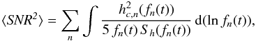 (A.1)where fn(t) indicates the frequency of the different harmonics at multiple integers of the orbital frequency (in our calculations, we adopt n = 1,...,20, which safely accounts for all the GW power) and is defined to be
  (where ν(t) is the orbital frequency and
  is the direction of pericentre with respect to
  – i.e. the vector product of the orbital angular momentum unit vector
  and the SMBH spin direction Ŝ). hc,n(fn(t)) is the characteristic amplitude and has been derived following Eq. (56) of Barack & Cutler (2004a; see also Cutler et al. 1993, 1994). Finally, Sh(fn(t)) accounts for the total noise of the interferometer and we give expressions for LISA, NGO and DECIGO in the next subsection. In this Paper, we derive fn(t) by solving, backwards in time, the system of differential post-Newtonian Eqs. (27–30) of Barack & Cutler (2004a). In particular, we evolve the mean anomaly Φ(t), the orbital frequency ν(t), the direction of pericentre and the orbital eccentricity e(t) starting from the LSO, backwards in time down to the assumed starting time of the observation. We define as t0 the duration elapsed between the starting time of the observation and the epoch when the companion reaches the LSO (in this paper, we consider four cases: t0 = 5, 6, 10 and 15 yr). We furthermore define Tmission the duration of the mission (in this paper, we consider two cases: Tmission = 5 and 2 yr). As arbitrary initial conditions, we set
  ,
,  , and we keep the LSO eccentricity eLSO as a free parameter (see Table 1), which yields
 ![Mathematical equation: \hbox{$\nu{}_{\rm LSO}=\left(2\,{}\pi{}m_{\rm SMBH}\right)^{-1}\,{}\left[\left(1-e^2_{\rm LSO}\right)/\left(6+2\,{}e_{\rm LSO}\right)\right]^{3/2}$}](/articles/aa/full_html/2012/06/aa18444-11/aa18444-11-eq184.png) .
.
Using the above equations, we can derive the luminosity distance DL(zmax(mSMBH, mco)) at which an event can be detected with a SNR ≥ 10 by a certain interferometer (see, e.g., Mapelli et al. 2010, and references therein). We can, thus, derive zmax(mSMBH, mco) by inverting the expression of the luminosity distance in a flat ΛCDM model:  (A.2)
(A.2)
A.1. LISA noise
Sh(fn(t)) accounts for the total noise of LISA noise and is defined as (Eq. (54) of Barack & Cutler 2004a):  (A.3)where
  is defined in Eq. (52) of Barack & Cutler (2004a; see also Hughes 2002) and accounts for both the instrumental noise (
 , Finn & Thorne 2000) and the Galactic confusion noise (
 , Nelemans et al. 2001; see also Bender & Hils 1997):
 ![Mathematical equation: \appendix \setcounter{section}{1} \begin{eqnarray} &&S_h^{\rm inst+gal}(f_n(t))=\textrm{min}\Bigg[\frac{S_h^{\rm inst}(f_n(t))}{\exp{(-\kappa{}\,{}T_{\rm mission}^{-1}\,{}N_f)}},\nonumber\\ &&S_h^{\rm inst}(f_n(t))+S_h^{\rm gal}(f_n(t))\Bigg], \end{eqnarray}](/articles/aa/full_html/2012/06/aa18444-11/aa18444-11-eq193.png) (A.4)where κ ~ 4.5 (Cornish 2003), Tmission is the duration of the mission, Nf = 2 × 10⁻³ Hz-1(Hz/fn(t))11/3 (Hughes 2002). is the same as in Eq. (48) of Barack & Cutler (2004a). is the same as in Eq. (51) of Barack & Cutler (2004a). Finally,
(A.4)where κ ~ 4.5 (Cornish 2003), Tmission is the duration of the mission, Nf = 2 × 10⁻³ Hz-1(Hz/fn(t))11/3 (Hughes 2002). is the same as in Eq. (48) of Barack & Cutler (2004a). is the same as in Eq. (51) of Barack & Cutler (2004a). Finally,  accounts for the extragalactic white dwarf background (Farmer & Phinney 2003) and is the same as in Eq. (50) of Barack & Cutler (2004a).
A.2. NGO noise
In the case of NGO, is defined as (Eq. (5) of Amaro-Seoane et al. 2012a): ![Mathematical equation: \appendix \setcounter{section}{1} \begin{eqnarray} S_h^{\rm inst}(f_n(t))&=&\frac{20}{3}\,{}\frac{4\,{}S_{\rm x,acc}(f_n(t))+S_{\rm x,sn}(f_n(t))+S_{\rm X,omn}(f_n(t))}{L^2}\nonumber\\ &&\quad\times \left\{1+\left[\frac{f_n(t)}{0.41\,{}\left(\frac{c}{2\,{}L}\right)}\right]^2\right\}, \end{eqnarray}](/articles/aa/full_html/2012/06/aa18444-11/aa18444-11-eq197.png) (A.5)where L = 109 m,
(A.5)where L = 109 m,  m2 Hz-1 is the power spectral density of the residual acceleration of the test mass, Sx,sn(fn(t)) = 5.25 × 10⁻²³ m2 Hz-1 is the shot noise power spectral density, and SX,omn(fn(t)) = 6.28 × 10⁻²³ m2 Hz-1 is the power spectral density of the other possible measurement noises.
As in the case of LISA, we combine the instrumental noise with the Galactic confusion noise and with the extragalactic white dwarf background (see Sect. A.1). On the other hand, the Galactic confusion noise and the extragalactic white dwarf background are negligible compared to in the case of NGO.
A.3. DECIGO noise
In the case of DECIGO, we calculate the noise as in Eq. (1) of Yagi & Tanaka (2010): ![Mathematical equation: \appendix \setcounter{section}{1} \begin{eqnarray} S_h(f_n(t))&=&\textrm{min}\Bigg[\frac{S_h^{\rm inst}(f_n(t))}{\exp{(-\kappa{}\,{}T_{\rm mission}^{-1}\,{}N_f)}},\,{}S_h^{\rm inst}(f_n(t))\nonumber\\ &&\quad +S_h^{\rm gal}(f_n(t)){\mathcal R}(f_n(t))\Bigg]+S_h^{\rm ex gal}(f_n(t)){\mathcal R}(f_n(t))\nonumber\\ &&\quad+0.01\,{}S_h^{\rm NS}(f_n(t)), \end{eqnarray}](/articles/aa/full_html/2012/06/aa18444-11/aa18444-11-eq204.png) (A.6)where the instrumental noise spectral density () is given by (Yagi & Tanaka 2010):
(A.6)where the instrumental noise spectral density () is given by (Yagi & Tanaka 2010): ![Mathematical equation: \appendix \setcounter{section}{1} \begin{eqnarray} S_h^{\rm inst}(f_n(t))&=&5.3\times{}10^{-48}\nonumber\\ &&\quad\times\left[(1+x^2)+\frac{2.3\times{}10^{-7}}{x^4(1+x^2)}+\frac{2.6\times{}10^{-8}}{x^4}\right]\,{}\textrm{Hz}^{-1}, \end{eqnarray}](/articles/aa/full_html/2012/06/aa18444-11/aa18444-11-eq205.png) (A.7)where x = fn(t)/fp with fp ≡ 7.36 Hz. κ, Tmission, Nf, and are the same as defined for LISA in Sect. A.1. Finally, the factor ℛ(fn(t)) ≡ exp [ − 2 (fn(t)/0.05Hz)2] represents the cutoff of the white dwarf-white dwarf binary confusion noise (Yagi & Tanaka 2010).
(A.7)where x = fn(t)/fp with fp ≡ 7.36 Hz. κ, Tmission, Nf, and are the same as defined for LISA in Sect. A.1. Finally, the factor ℛ(fn(t)) ≡ exp [ − 2 (fn(t)/0.05Hz)2] represents the cutoff of the white dwarf-white dwarf binary confusion noise (Yagi & Tanaka 2010).
Appendix B: Estimate of p from the Press-Schechter formalism
We can derive p in the following way. Driver et al. (2007) estimate that the current stellar mass density of spheroids is  (where h = 0.71, Larson et al. 2011). Using the Schechter function (see Driver et al. 2007 for details), we find that the mass fraction of spheroids with mass 108 ≤ msph/M⊙ ≤ 1010 is g ~ 0.34. Thus, the current mass density of halos hosting spheroids with mass 108 ≤ msph/M⊙ ≤ 1010 is
  (B.1)where f∗ is the fraction of baryons in stars, ρdisc is the current stellar mass density of discs,
  and
and  (Larson et al. 2011). Assuming g = 0.34, f∗ = 0.119 h and ρdisc = 4.4 × 10⁸h M⊙ Mpc-3 (from Driver et al. 2007), we find
  .
.
A density can be obtained by integrating the Press-Schechter function (Press & Schechter 1974; Eisenstein & Hu 1998, 1999) between mh1 = 9.44 × 10⁹ M⊙ and mh2 = 9.44 × 10¹¹ M⊙ (which satisfies the further requirement that mh2 = 100 mh1). mh1 = 9.44 × 10⁹ M⊙ and mh2 = 9.44 × 10¹¹ M⊙ can be used as integration limits in Eq. (5). Finally, we can derive also the value of p as p = msph1/mh1 = 1.06 × 10⁻².
We note that this value of p matches very well with the observations of the Milky Way, but there may be large deviations from it, depending on the morphological type (see, e.g., Graham & Worley 2008). A different value of p may significantly affect the results (see the examples in Tables 1–3).
All Tables
All Figures
|
Fig. 1 zmax in the case of LISA, as a function of mSMBH for three different simulations. In all the shown models, j = 1 and Tmission = t0 = 5 yr (see Table 1). Solid line (red on the web): model with eLSO = 0.3. Dashed line (blue on the web): model with eLSO = 0.5. Dotted black line: model with eLSO = 0.7. |
| In the text | |
|
Fig. 2 zmax in the case of NGO, as a function of mSMBH for three different simulations. In all the shown models, j = 1 and Tmission = t0 = 5 yr (see Table 2). Solid line (red on the web): model with eLSO = 0.3. Dashed line (blue on the web): model with eLSO = 0.5. Dotted black line: model with eLSO = 0.7. |
| In the text | |
|
Fig. 3 zmax in the case of DECIGO, as a function of mSMBH for three different simulations. In all the shown models, j = 1 and Tmission = t0 = 5 yr (see Table 3). Solid line (red on the web): model with eLSO = 0.3. Dashed line (blue on the web): model with eLSO = 0.5. Dotted black line: model with eLSO = 0.7. |
| In the text | |
|
Fig. 4 The total detection rate R versus the adopted eccentricity at the LSO (eLSO), in the case of LISA (filled circles, red on the web), DECIGO (filled triangles, blue on the web) and NGO (filled squares). For each case, j = 1, t0 = 5 yr, Tmission = 5 yr (see Tables 1–3), p = 1.06 × 10⁻², |
| In the text | |
|
Fig. 5 Cumulative redshift distribution of the expected detections per year, in the case of LISA (dotted line, red on the web), DECIGO (dashed line, blue on the web) and NGO (solid line). For each case, j = 1, eLSO = 0.1, t0 = 5 yr, Tmission = 5 yr (see Tables 1–3), p = 1.06 × 10⁻², |
| In the text | |
Current usage metrics show cumulative count of Article Views (full-text article views including HTML views, PDF and ePub downloads, according to the available data) and Abstracts Views on Vision4Press platform.
Data correspond to usage on the plateform after 2015. The current usage metrics is available 48-96 hours after online publication and is updated daily on week days.
Initial download of the metrics may take a while.