| Issue |
A&A
Volume 542, June 2012
|
|
|---|---|---|
| Article Number | A76 | |
| Number of page(s) | 12 | |
| Section | Interstellar and circumstellar matter | |
| DOI | https://doi.org/10.1051/0004-6361/201118413 | |
| Published online | 12 June 2012 | |
The massive protostar W43-MM1 as seen by Herschel-HIFI water spectra: high turbulence and accretion luminosity⋆,⋆⋆
1
Univ. Bordeaux, LAB, UMR 5804, 33270
Floirac,
France
e-mail: This email address is being protected from spambots. You need JavaScript enabled to view it.
2
CNRS, LAB, UMR 5804, 33270
Floirac,
France
3
SRON Netherlands Institute for Space Research,
PO Box 800, 9700AV
Groningen, The
Netherlands
4
Max-Planck-Institut für Radioastronomie,
Auf dem Hügel 69, 53121
Bonn,
Germany
5
Leiden Observatory, Leiden University,
PO Box 9513, 2300 RA
Leiden, The
Netherlands
6
Max Planck Institut für Extraterrestrische Physik,
Giessenbachstrasse 1,
85748
Garching,
Germany
Received: 7 November 2011
Accepted: 2 April 2012
Abstract
Aims. We present Herschel-HIFI observations of 14 water lines in W43-MM1, a massive protostellar object in the luminous star-cluster-forming region W43. We place our study in the more general context of high-mass star formation. The dynamics of these regions may be represented by either the monolithic collapse of a turbulent core, or competitive accretion. Water turns out to be a particularly good tracer of the structure and kinematics of the inner regions, allowing an improved description of the physical structure of the massive protostar W43-MM1 and an estimation of the amount of water around it.
Methods. We analyze the gas dynamics from the line profiles using Herschel-HIFI observations acquired as part of the Water In Star-forming regions with Herschel project of 14 far-IR water lines (H216O, H217O, H218O), CS(11–10), and C18O(9–8) lines, using our modeling of the continuum spectral energy distribution. The spectral modeling tools allow us to estimate outflow, infall, and turbulent velocities and molecular abundances. We compare our results to previous studies of low-, intermediate-, and other high-mass objects.
Results. As for lower-mass protostellar objects, the molecular line profiles are a mix of emission and absorption, and can be decomposed into “medium” (full width at half maximum FWHM ≃ 5–10 km s-1), and “broad” velocity components (FWHM ≃ 20–35 km s-1). The broad component is the outflow associated with protostars of all masses. Our modeling shows that the remainder of the water profiles can be well-fitted by an infalling and passively heated envelope, with highly supersonic turbulence varying from 2.2 km s-1 in the inner region to 3.5 km s-1 in the outer envelope. In addition, W43-MM1 has a high accretion rate of between 4.0 × 10⁻⁴ and 4.0 × 10⁻² M⊙ yr-1, as derived from the fast (0.4–2.9 km s-1) infall observed. We estimate a lower mass limit for gaseous water of 0.11 M⊙ and total water luminosity of 1.5 L⊙ (in the 14 lines presented here). The central hot core is detected with a water abundance of 1.4 × 10⁻⁴, while the water abundance for the outer envelope is 8 × 10⁻⁸. The latter value is higher than in other sources, and most likely related to the high turbulence and the micro-shocks created by its dissipation.
Conclusions. Examining the water lines of various energies, we find that the turbulent velocity increases with the distance from the center. While not in clear disagreement with the competitive accretion scenario, this behavior is predicted by the turbulent core model. Moreover, the estimated accretion rate is high enough to overcome the expected radiation pressure.
Key words: ISM: molecules / ISM: abundances / stars: formation / stars: protostars / stars: early-type / line: profiles
Herschel is an ESA space observatory with science instruments provided by European-led Principal Investigator consortia and with important participation from NASA.
HIFI data is only available at the CDS via anonymous ftp to cdsarc.u-strasbg.fr (130.79.128.5) or via http://cdsarc.u-strasbg.fr/viz-bin/qcat?J/A+A/542/A76
© ESO, 2012
1. Introduction
After hydrogen and helium, oxygen is the most abundant element in the Universe and water is one of the most abundant molecules. Owing to the water in the Earth’s atmosphere, space-based observations are necessary to study the vast majority of the water transitions. Because of its importance to life and its sensitivity to dynamical, thermal, and chemical processes in the interstellar medium, the physics and chemistry of water is one of the main drivers of the Herschel space observatory mission (hereafter Herschel, Pilbratt et al. 2010) and particularly of the HIFI spectroscopy instrument (de Graauw et al. 2010).
Massive stars are rare but are the major contributors to the matter cycle in the Universe owing to their short lifetimes and rapid ejection of enriched material. The OB stars dominate the energy budget of star-forming galaxies and are visible at large distances. Their formation, however, is not well-understood and the classical scheme for low-mass star formation cannot be applied as such to OB stars. Indeed, young OB stars and protostars strongly interact with the surrounding massive clouds and cores, leading to a complex and still not clearly defined evolutionary sequence. We generally identify in this sequence objects ranging from massive pre-stellar cores, high-mass protostellar objects (HMPOs), hot molecular cores (HMC), and finally to the more evolved uItra compact HII region stage, where the central object begins to ionize the surrounding gas (e.g., Beuther et al. 2007). The classification adopted above is not unique but is consistent with the analysis of massive young stellar objects and HII regions in the Galaxy made by Mottram et al. (2011). The most problematic issue in understanding the massive-star formation process is to explain how to accumulate a large amount of mass infalling within a single entity despite radiation pressure. Models considering a protostar-disk system (e.g., Yorke & Sonnhalter 2002; Krumholz et al. 2005; Banerjee & Pudritz 2007) now quite successfully address how the accretion of matter overcomes radiative pressure. Two main theoretical scenarios have been proposed to form high-mass stars, which both require the presence of a disk and high accretion rates: (a) a turbulent core model with a monolithic collapse scenario (Tan & McKee 2002; McKee & Tan 2003); and (b) a highly dynamical competitive accretion model involving the formation of a cluster (Bonnell & Bate 2006). In ionized HII regions, star formation could also be triggered by successive generations of stars (e.g., Deharveng et al. 2009). One of the implications of the turbulent core model is that molecular line profiles should have supersonic turbulent widths, while the competitive accretion produces cores that are subsonic, hence have a rather small amount of turbulence (see Krumholz & Bonnell 2009). In the deeply embedded phase of star formation, it is only possible to trace the dynamics of gas using resolved emission-line profiles, similar to those obtained with HIFI.
The guaranteed-time key program Water In Star-forming regions with Herschel (WISH, van Dishoeck et al. 2011) probes massive-star formation using water observations performed by the HIFI and PACS (Poglitsch et al. 2010) instruments. In particular, we characterize the dynamics of the central regions using the water lines and measure the amount of cooling that provide. In molecular clouds, water is mostly found as ice on dust grains, but at temperatures T > 100 K the ice evaporates, increasing the gas-phase water abundance by several orders of magnitude (Fraser et al. 2001; Aikawa et al. 2008). This suggests that water emission almost exclusively probes the warm inner regions of protostellar objects. To collapse, the gas must be able, among several other conditions, to release enough thermal energy; a major WISH goal is to determine how much of the cooling of the warm region (T > 100 K) is due to H2O.
The high velocity resolution of the HIFI instrument allows us to study the dynamics of the gas, detect outflows, and estimate the infall and turbulent velocities present in the protostellar envelopes. Even though the water abundance in the envelope is low, low energy lines are highly absorbed by the envelope, producing a mixture of emission and absorption that can nevertheless be resolved at the spectral resolution of HIFI. The high-energy lines are observed in emission and directly probe the warm regions since their lower energy levels are not excited in the envelope, and as such cannot absorb emission from the hot core. Thus, observations of a mixture of low- and high- lying lines of water and its isotopologues allow us to perform a “tomography” of the structure of protostellar envelopes.
A first review of WISH and its results was presented and compiled by van Dishoeck et al. (2011) for only a few objects. We expect to confirm these results by studying of the whole sample. Interestingly, the water line profiles (transitions p-H2O 111–000 and p-H2O 202–111) obtained in a low- (NGC 1333, Kristensen et al. 2010), an intermediate- (NGC 7129, Johnstone et al. 2010), and a high-mass (W3IRS5, Chavarría et al. 2010) young stellar object (YSO) exhibit similar velocity components: a broad (full width at half maximum FWHM ~25 km s-1) and a medium (~5–10 km s-1) one. A narrower component (<5 km s-1) is also observed, but not in the massive object, although it was detected toward W3IRS5 by Wampfler et al. (2011) based on its the OH emission. The water emission differs in terms of intensity, the massive objects being the strongest emitters. Another high-mass star-forming region, DR21(Main) was studied by van der Tak et al. (2010) in the para ground-state water and 13CO lines. They derived a very low water abundance of a few 10-10 in the outer envelope, and a higher one by nearly three orders of magnitude in the outflow (7 × 10⁻⁷). Water abundance estimates toward four other massive YSOs were made by Marseille et al. (2010b) using the lowest two p-H2O lines combined with the ground state p-H O line. Variations in the outer envelope water abundance were measured (from 5 × 10⁻¹⁰ to 4 × 10⁻⁸), but are not correlated with either the luminosity or evolutionary stage. Finally, no infall has ever been firmly established for these objects.
In this paper, we analyze the water observations toward the massive dense core W43-MM1 in the mini-starburst region W43, located near the end of the Galactic bar at a distance of 5.5 kpc (Motte et al. 2003; Nguyen Luong et al. 2011). This region is one of the most interesting star-formation regions in several aspects (e.g., Bally et al. 2010). It has a star-forming rate that has increased by an order of magnitude in the past ~106 years (Nguyen Luong et al. 2011). The source is an IR-quiet dense core based on the definition of Motte et al. (2007) with bolometric luminosity 2.3 × 10⁴L⊙ and size of 0.25 pc. This massive dense core is expected to be fragmented on small scales and should be considered as a protocluster. W43-MM1 is the most massive dense core (M ~3600 M⊙, Motte et al. 2003) of the four identified main millimeter fragments of which only MM1 is within the HIFI beam. The mid-IR emission from the hot core is undetected because it is totally absorbed by the envelope, while the source is detected at 24 μm (peak flux = 0.3 Jy). A methanol and a water maser are detected but there is neither near-infrared nor centimeter emission. Infall (up to 2.9 km s-1) was identified by Herpin et al. (2009) from CS data. W43-MM1 resembles a low-mass Class 0 protostar, i.e., a YSO in its main accretion phase, but scaled up in mass and luminosity. However, although it resembles a very young mid-IR quiet HMPO, W43-MM1 has already developed a hot core with temperatures higher than 200 K (Motte et al. 2003; Marseille et al. 2010b), making this object very peculiar. All of these characteristics make W43-MM1 a promising massive object to study, that is potentially rich in water: among the first ten massive sources, from different evolutionary stages, observed by Marseille et al. (2010a), W43-MM1 is one of only three sources (i.e. in addition to DR21OH and IRAS 18089-1732) to be detected in the p-HO 313–320 line.
We present here new Herschel-HIFI observations of 14 far-IR water lines (H O, H
O, H O, HO), providing the most complete coverage of the water energy ladder to date, plus CS(11–10) and C18O(9–8) data. Sections 2 and 3 present our observations and results, whose analysis is given in Sect. 4. We then model the observations using a radiative transfer code in Sect. 5. We estimate the outflow and infall velocities, turbulent velocity, molecular abundances, and the physical structure of the source. We finally discuss (Sect. 6) the results in terms of massive-star formation scenarios.
Herschel-HIFI observed line transitions in W43-MM1. Frequencies are from Pearson et al. (1991). Beam and ηmb are from Roelfsema et al. (2012). The rms is the noise at the given spectral resolution δν.
2. Observations
Fourteen water lines as well as the CS(11–10) and C18O(9–8) lines (see Table 1) have been observed with HIFI at frequencies between 538 GHz and 1670 GHz toward W43-MM1 in March, April, and October 2010 (OD 293, 295, 310, 312, 333, 338, 339, and 531). The position observed corresponds to the peak of the mm continuum emission from Motte et al. (2003) (RA = 18:47:47.0, Dec = −01:54:28 J2000). The observations are part of WISH.
Data were taken simultaneously in H and V polarizations using both the acousto-optical Wide-Band Spectrometer (WBS) with a 1.1 MHz resolution and the digital auto-correlator or High-Resolution Spectrometer (HRS) providing higher spectral resolution. We used the double beam switch observing mode with a throw of 3′. The HIFI receivers are double sideband with a sideband ratio close to unity. The frequencies, energy of the upper levels, system temperatures, integration times, and rms noise level at a given spectral resolution for each of the lines are provided in Table 1. The calibration of the raw data onto the TA scale was performed by the in-orbit system (Roelfsema et al. 2012); and the conversion to Tmb was done using a beam efficiency given in Table 1 and a forward efficiency of 0.96. The flux scale accuracy was estimated to be 10% for bands 1 and 2, 15% for bands 3 and 4, and 20% in bands 6 and 7. Data calibration was performed in the Herschel Interactive Processing Environment (HIPE, Ott 2010) version 6.0. Further analysis was done within the CLASS1 package. These lines are not expected to be polarized, thus, after inspection, data from the two polarizations were averaged together. For all observations, we checked for any eventual contamination from lines in the image sideband of the receiver but none was found. Since HIFI operates in double-sideband, the measured continuum level (in the figures and the tables) was divided by a factor of two.
3. Results
The spectra including continuum emission are shown in Figs. 1 and 2 for the rare isotopologues (HO, HO) and HO, respectively. In addition, Fig. 3 displays the CS (11–10) and C18O (9−8) spectra. We show the HRS spectra, except for the p-HO 111–000, o-HO 212–101, p-H2O 202–111, p-H2O 111–000, o-H2O 221–212, and o-H2O 212–101 lines, where WBS spectra were used since the velocity range covered by the HRS was insufficient.
We derived the peak main-beam temperatures and half power line-widths for the different line components from multi-component Gaussian fits, made with the CLASS software (line parameters are given in Table 2). All lines associated with the source have Vlsr ≃ 95−100 km s-1. Since W43-MM1 is located in a very crowded area of the Galactic plane (b ~− 0.1°), foreground clouds contribute to the spectra in terms of water absorption at Vlsr shifted with respect to W43 velocity in the o-H2O 110–101, p-H2O 111–000 and o-H2O 212–101 lines spectra. These are discussed in Appendix A.
As in Johnstone et al. (2010), Kristensen et al. (2010), and Chavarría et al. (2010), we adopt the following terminology for the different velocity components: broad (FWHM ≃ 20–35 km s-1), medium (FWHM ≃ 5–10 km s-1), and narrow (~3 km s-1).
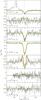 |
Fig. 1 HIFI spectra of H |
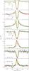 |
Fig. 2 HIFI spectra of H |
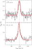 |
Fig. 3 Continuum-subtracted HIFI spectra of the C18O 9–8 and CS 11–10 lines (in black). The model fits are shown as red lines over the spectra. Vertical dotted lines indicate the VLSR at 99.4 km s-1. The spectra have been smoothed to 0.2 km s-1. The unidentified line in absorption seen at 88.6 km s-1 is indicated. |
3.1. C-bearing species
Although the main goal of WISH is to observe H2O, the HIFI bands included the C18O (9–8) and CS (11–10) lines. They are seen in emission without any broad component contribution. While the source velocity derived by Motte et al. (2003) from H13CO+ observations is 98.8 km s-1, the best-fit Gaussian for the observed C18O (9–8) line emission is centered at 99.4 km s-1 (with a FWHM of 5.6 km s-1), which is consistent taking into account the uncertainties. The CS 11–10 line profile is most closely fit by two Gaussians of widths 2.9 km s-1 and 10.2 km s-1, centered at 98.4 and 98.8 km s-1, respectively, but the CS line profile is asymmetric, which is possibly indicative of infall that blue-shifts the emission peak. In the following, we adopt Vlsr = 99.4 km s-1 as the source velocity.
We note that an unidentified line is detected in absorption in the C18O (9–8) spectra at 88.6 km s-1, i.e., 987.594/ 972.747 GHz in upper/lower side-band.
3.2. H216O lines
Most of the HO lines can be described as the sum of a medium (FWHM ≃ 5–10 km s-1) and a broad (up to 35 km s-1) velocity components. The broad one is likely the signature of an outflow. The observed dependence of the outflow velocity extent on Eup is probably due to sensitivity effects (the outflow being more difficult to detect at weaker line intensity). The medium component is centered at 99.4–99.9 km s-1 (fitting uncertainty), while the broad one is redshifted by a few km s-1 from the source velocity. The main water line profiles are more complex than those of the rare isotopologues. Except for the o-H2O 221–212, p-H2O 211–202, and o-H2O 312–303 lines, none of the spectra exhibit pure absorption or emission line profiles.
For low-mass objects, Kristensen et al. (2010) interpreted the narrow emission as the signature of the passively heated envelope, while the medium component might be due to shocks, but on spatial scales smaller than the molecular jets; the broad emission arises in the extended molecular outflow.
The para and ortho ground-state lines are deeply absorbed but their profiles also exhibit a broad outflow component. The o-H2O 110–101 and p-H2O 111–000 line profiles are fully absorbed as is more or less the o-H2O 212–101 line, while the peak depth of the o-H2O 221–212 line is 1.1 K (~65% of the continuum level, see Table 2). The p-H2O 202–111 line profile is also dominated by an absorption dip at 1.6 K (~11% of the continuum), but has a strong (up to 1K) and broad outflow (21 km s-1) component. This line is actually the most sensitive to the outflow.
Except for the o-H2O 221–212 line with an Eup at 194 K that is seen in absorption, the emission lines involving energy levels above 130 K reveal an infall signature characterized by an asymmetrical profile with a stronger blue component than the red one (see for example the p-H2O 211–202 spectra).
3.3. Rare water isotopologues
Among all observed HO and HO lines, the o-HO 110–101 and p-HO 202–111 lines are not detected (assuming a line width of 6 km s-1, upper limits are 280 and 650 mK km s-1, respectively). The o-HO 312–303 line is tentatively detected at the 2σ level.
The observed profiles of lines related to either a ground-state ortho or para level are dominated by absorption from the cold outer envelope. This is a bit surprising as one would have expected at least the o-HO 212–101 to be in emission because of the high energy level involved. All these absorptions are centered at 99.6 ± 0.3 km s-1and can be fit by a single Gaussian with a velocity width ranging from 4.7 to 6.4 km s-1, corresponding to our “medium” component. No broad component is observed. Line parameters are given in Table 2.
Observed line-emission parameters for the detected lines. νLSR is the line peak velocity.
4. Analysis
4.1. Line asymmetries
Outflows, infall, and rotation can produce very specific line profiles with characteristic signatures (see Fuller et al. 2005, and references therein). Outflow and rotation give rise to both red and blue asymmetric lines, while the profiles of optically thick lines from infalling material have stronger blue-shifted emission than the redshifted emission. However, in some circumstances, outflow or rotation could also produce a blue asymmetric line-profile along a particular line of sight to the source.
Compared to the C18O (9–8) optically thin line (ν = 99.4 km s-1), several water-line profiles show clear asymmetry. Focusing our analysis on emission lines, strong asymmetries are detected in the p-H2O 211–202 and o-H2O 312–303 lines. Both profiles clearly exhibit a stronger blue component which is presumably indicative of infall. Strong asymmetries were previously measured in the CS line profiles (involving lower energy levels) toward this source by Herpin et al. (2009), and the CS 11–10 line observed here also exhibits an infall signature.
The absorption lines (including the rare isotopologues) do not show clear asymmetry, but as indicated by the absorption peak velocities (see Table 2), several of them are indeed redshifted (relative to the source velocity of 99.4 km s-1), as expected in the case of infall.
The p-H2O 202–111 line profile, which has a very slightly stronger blue peak than the red one, exhibits a strong self-absorption dip at the source velocity. This almost symmetric double-horn profile might be produced by the outflow (Fuller et al. 2005). In reality, the absorption is seen against both the outflow and continuum emission. Hence, as shown by Kristensen et al. (in press), the outflow is also embedded (i.e., the absorption layer is in front of both of the emitting layers).
4.2. Opacities
For the absorption lines, we estimated the opacities at the maximum of absorption from the line-to-continuum ratio in Table 2 using the formula  (1)and assuming that the continuum is completely covered by the absorbing layer.
The HO lines are somewhat optically thick, with τ ≈ 0.2–0.3, if we exclude the tentatively detected o-HO 312–303 line. In contrast, the HO lines are close to being optically thin, with τ ≈ 0.1.
Of the HO lines detected in absorption, all but the p-H2O 202–111 line are highly optically thick. We note that the optical depth of this line may be (much) higher if not only continuum but also line emission is absorbed (see van der Tak et al., in prep.). The o-H2O 110–101, p-H2O 111–000, and o-H2O 212–101 line profiles display absorption nearly down to the zero-temperature level, leading to opacities larger than three in the coolest shells. All of these types of absorption are due to the cold material in which the protostar is embedded.
5. Modeling
In the preceding sections, we have demonstrated how the line profiles can be decomposed into various dynamical components empirically and how their asymmetry can be indicative of infall. We now present our model for the full line profiles in a single spherically symmetric model with different kinematical components due to turbulence, infall, and outflow.
5.1. Method
We used the two-dimensional (2D) Whitney-Robitaille radiative transfer code (hereafter WR, Whitney et al. 2003; Robitaille et al. 2006, 2007) to derive the envelope temperature and density profiles. The physical model consists of a spherical envelope with neither disk nor cavity to emulate a one-dimensional (1D) model. The density decreases exponentially with radius and follows the relation 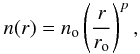 (2)where no = 5.77 × 106 cm-3 is the number density at a radius ro = 1 × 10⁴ AU for the derived envelope mass. We assumed a p value of −1.5 (model parameters are listed in Table 3). Dust opacities (with thin ice coated grains) were taken from Ossenkopf & Henning (1994). The envelope temperature and mass were constrained by comparing the WR-derived spectral energy distribution (SED) with existing sub-millimeter continuum fluxes (see Fig. 5) inferred from our Herschel observations and those of Bally et al. (2010), the CSO/SHARC and IRAM/MAMBO observations of Motte et al. (2003), JCMT/SCUBA and Spitzer-MIPS archival data (see Fig. 5), and KAO observations (Lester et al. 1985). Observed peak fluxes were normalized to the source size (55 000 AU ≃ 10′′ at 5.5 kpc) derived from 1.2 mm continuum at 3σ standard deviation above the noise level (Motte et al. 2003).
The line emission were modeled using the 1D radiative transfer code RATRAN (Hogerheijde & van der Tak 2000) using the WR-derived envelope temperature and density profiles (see Fig. 4), following the method described in Marseille et al. (2008) and Chavarría et al. (2010). The H2O collisional rate coefficients were taken from Faure et al. (2007).
Parameters used in Whitney-Robitaille continuum model and derived physical quantities.
Our model of W43-MM1 has two components: an outflow and the proto-stellar envelope. The outflow parameters (intensity, velocity width) were derived from the Gaussian fitting of the emission lines, which have FWHMs between 10.2 and 35.5 km s-1 depending on the line. We used RADEX (van der Tak et al. 2007) to estimate the H2O column density and opacity in the outflow. To retrieve the observed intensities for the outflow component, we adopted Tkin = 100 K and n(H2) = 107 cm-3 (following the density profile shown in Fig. 4), and a water column density of 1014 cm-2. Since RATRAN only enables us to include the outflow as an additional component (with T, opacity, and width), that is not part of the radiative transfer process, the outflow component was assumed to be an unrelated component, both spatially and in velocity space. The result was directly incorporated into the ray-tracing part of the RATRAN code (see Hogerheijde & van der Tak 2000). As a consequence, we stress that the absorption in the modeled line profile is very likely overestimated, i.e., the cold layer in size or temperature.
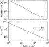 |
Fig. 4 Density and temperature profile derived from SED modeling. |
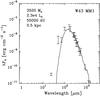 |
Fig. 5 Spectral energy distribution for W43-MM1 calculated using the Whitney-Robitaille model for the parameters in Table 3. Error bars are from the references cited in Sect. 5.1. |
The envelope contribution was parametrized with three input variables: water abundance (χH2O), turbulent velocity (Vtur), and infall velocity (Vinfall). The width of the line was adjusted by varying Vtur. The line asymmetry was reproduced by the infall velocity Vinfall. The line intensity was most closely fitted by adjusting a combination of the abundance and both the Vtur and Voutflow parameters. We adopted the following standard abundance ratios for all the lines: 450 for HO/HO, 4.5 for HO/HO (Wilson & Rood 1994; Thomas & Fuller 2008), and 3 for ortho/para-H2O. The models assumed a jump in the abundance in the inner envelope at 100 K (see Sect. 5.4). Table 4 gives the parameters used in the models.
To fit the observed lines, we first modeled the rare isotopologues (HO, then HO) lines and the HO line, which involves the highest energy level (o-H2O 312–303; optically thin), using the same abundances for all lines (the HO abundances were derived from the HO and HO values times the isotopic abundance ratios). Once we were able to reproduce the main features of the profiles by minimizing the residuals in a grid of values, we modeled the remaining lines using the same parameters, including the outflow component when this is justified.
We simultaneously used two different criteria to quantify the quality of our model:
-
We quantified the error ε relative to the intensity T and width Δv of the line
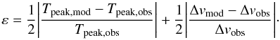 (3)
(3) -
The similarity between the observed and the modeled line profiles was quantified by comparing for each channel the observed (Ti) and modeled intensities (Ti ⋆ ) (above the 3σ detection limit). We defined a detection function Di and a correlation function Ci to be
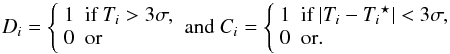 (4)The
computed parameter was called the profile similarity factor Σ
(4)The
computed parameter was called the profile similarity factor Σ 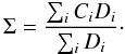 (5)
(5)
Physical quantities derived from the RATRAN model.
5.2. Velocity structure
To constrain the source dynamics, we followed two different approaches: 1) a model with constant turbulent velocity and zero infall (Vtur = 2.5 km s-1 and Vinfall = 0.0 km s-1) for all lines and all radii, and 2) a model in which the velocity parameters vary with radius. An inspection of the line profiles (see Sect. 3) shows that for all lines there is neither identical velocity component widths, nor identical infall contributions, so we do not expect a model with equal velocity parameters for all lines to fit the data well. For most of the lines, the model 1 (see Figs. 1 and 2) indeed fails to reproduce the global shapes of the profiles, especially those of HO.
The best-fit model has both turbulence and infall that vary with radius (see Figs. 1 and 2), as already seen by Caselli & Myers (1995) for the turbulence. We first tried to apply a power-law variation for both parameters but without any success. We also unsuccessfully tried a “two-step” turbulence (Vtur = 2.2 km s-1 up to a certain radius, i.e., around 104 AU, and beyond 3.5 km s-1). Adopting “multiple-step profile” (Fig. 6) for the turbulence provided much tighter fits for all line profiles with the same model. The infall was also most tightly constrained by a step function given in Fig. 6. Each shell of the envelope (at radius R) was hence characterized by a temperature, a density, turbulence, and an infall velocity as shown in Figs. 4 and 6. We estimated the uncertainties in these velocities by allowing the velocity to vary around the best-fit values at each radius.
 |
Fig. 6 Variation in the turbulent and infall velocities, respectively Vturb and Vinf, with the radius R (AU) to the central object. We overplot the radii corresponding to the temperature jump (dashed) in the model and to the radius where lines of different energies originate mainly from the upper energy levels as dashed lines. |
Line profiles for all species are well-reproduced by our model (Figs. 1–3), with Σ similarity coefficient larger than 90%, and ε and χ2 were minimized for most lines (o-HO 110–101, p-H2O 211–202, and o-H2O 110–101 have Σ ≃ 75%), even with an outflow contribution fit with a simple Gaussian model. These model predictions are consistent with the upper limits to the non-detected lines o-HO 110–101 and p-HO 202–111, and the tentatively detected o-HO 312–303 line. The CO and CS lines are well-reproduced by the model derived from the other lines. All modeled lines are centered on a VLSR equal to 99.4 km s-1, but the outflow component central velocity varies somewhat from line to line by ±0.5−1.0 km s-1. In addition, we applied our model to the HO 313−220 line at 203.3916 GHz (Eup = 204 K) observed with the IRAM-30 m telescope (ΔV = 3.8 km s-1) by Marseille et al. (2010a), finding that the line profile is perfectly reproduced.
5.3. Infall and accretion rate
Both outflow (e.g., Walker et al. 1988) and rotation (Zhou 1995; Fuller et al. 2005) can also produce blue asymmetric lines along a particular line of sight to the source. Hence, since blue asymmetry is observed in several water transitions (see also Herpin et al. 2009, for CS), and there is no evidence of contradictory information in the form of red asymmetric profiles, the infall explanation is the most likely. Nevertheless, only mapping (and a position-velocity diagram study) with a high angular resolution (of a few 0.1 arcsec) could help us to distinguish the effects of rotation and infall. Rotation might indeed produce a symmetry reversal in the outer parts in the direction perpendicular to the rotational axis, where the optical thickness is less (Zhou 1995; Yamada et al. 2009).
From the infall velocity Vinfall, we estimated the mass accretion rate Ṁacc by applying the method described by Beltrán et al. (2006). As a first rough estimate, we assumed that the gas is undergoing spherically symmetric free-fall collapse onto the central object. At any radius R, the mass accretion rate is given by 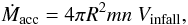 (6)where m is the mean molecular mass, n the gas volume density, and Vinfall the infall velocity at R as shown in Fig. 6.
The maximum infall velocity of 2.9 km s-1 is derived mainly from the p-H2O 211–202 and o-H2O 312–303 line profiles. From the model (Fig. 6 and Sect. 5.2), we can infer from the infall velocity that the corresponding radius from the protostar is 5.7−7.3 × 1017 cm (38 100–48 800 AU). The inferred mass accretion rate for this range of radii is then 3.5 to 4.0 × 10⁻² M⊙ yr-1, which is slightly lower by a factor of two than the value derived by Herpin et al. (2009) from CS observations. At such radii, we probably measure the accretion from the envelope toward the disk, if there is indeed a disk. However, according to our model, the infall velocity varies with radius, i.e., the mass accretion rate is not constant with radius. Within a radius of 26 800 AU, the infall velocity is only 0.4 km s-1, which leads to a mass accretion rate of between 4.0 × 10⁻⁴ and 5.0 × 10⁻³ M⊙ yr-1.
5.4. Abundance structure
Modeling the whole set of observed lines allows us to determine the abundance structure. Among the lines that are mostly excited in the inner envelope, only the higher-J HO (o-HO 312–303 and p-HO 313–320) and the o-H2O 312–303 lines are sufficiently optically thin to probe the inner parts of the envelope. To reproduce these lines, an abundance jump at 100 K is necessary but not for the remaining lines. The derived HO abundance relative to H2 is 1.4 × 10⁻⁴ in the warm part of the envelope where T > 100 K, while it is 8.0 × 10⁻⁸ in the outer parts where T < 100 K, in agreement with the values found by Marseille et al. (2010a) from HO observations. No deviation from the standard o/p ratio of 3 at high temperature (≥ 100 K) is found. Hence, the 1D approach seems acceptable as the shapes of all line profiles are well recovered.
From the integrated fluxes given in Table 2 (measured for the lines at least partly in emission), one can derive the water luminosities. We then estimate, assuming isotropic radiation and a distance of 5.5 kpc, that the minimum total HIFI water luminosity is 1.5 L⊙ (equal to the sum of all individual observed luminosities). The true water emission from the inner parts might be much greater but the cool envelope absorbs much of the emission. Moreover, from the modeling we estimate the total water (radial) column density in the envelope to be 1.56 × 1021 cm-2, corresponding to 0.11 M⊙ ( M⊙ and
  M⊙). More than 97% of this mass resides in the inner parts. The CS and C18O column densities are respectively 7.3 × 10¹⁵ and 8.2 × 1017 cm-2, leading to masses of 3.2 × 10⁻⁴ (CS) and 1.0 × 10⁻² (C18O, 5.0 for CO) M⊙. Hence the mass of oxygen trapped in H2O and CO is around 3 M⊙, that locked in CO 96%, and in H2O 4%.
5.5. Uncertainties and robustness of the parameters
The uncertainties in our calculations originate from three main sources:
-
the intensity calibration of the observed lines (seeSect. 2);
-
the physical limits of our model, whose radiative transfer computations are based on a physical description of the source derived from 1D SED modeling;
-
the parameter sensitivity of the line radiative-transfer model.
We rerun the models by first increasing, then decreasing the observed line intensities by the uncertainties given in Sect. 2. We found that the differences in the estimated abundances were between 10% and 30% depending on the line. To test the influence of the physical model, we decreased the envelope mass by 30% (which gives an SED just below the error limits) and recalculated the water abundances. We found differences of up to 75%. In addition, since the error in the exponent of the density profile is 0.1 (see Sect. 5.1), we tested the robustness of our results by varying the density profile within that range: we found that the abundances can vary by 30–40%. Moreover, the uncertainty in the distance to the source (we adopt 5.5 kpc, but Nguyen Luong et al. 2011, place the distance at 5.9 kpc) translates into an uncertainty in the physical model: an uncertainty of 10% in the distance leads to one of 15% in the mass hence 30% in the abundance. This of course impacts our results. In addition, we checked that varying the best-fit parameters from Table 4 by 5% has no influence on the derived abundances. A variation in the turbulent velocity within the error bars (and by varying the radius by 15%) shown in Fig. 6 does not affect our results. This value of turbulent velocity, as explained in Sect. 5.2, is well-constrained thanks to the large number of observed lines, which efficiently probe different radius. The determination of the infall velocity versus the radius is more uncertain because the infall signature is invisible for the quite completely absorbed lines.
Unfortunately, we are unable to determine wether these uncertainties are independent of each other. Hence, only the uncertainties coming from the HIFI intensity calibration provide us with a realistic quantitative estimate of the impact on our calculations. In an upcoming study, we plan to investigate how a 2D model incorporating a disk and a cavity (e.g., Hosokawa et al. 2010) would affect our results presented here. That the spherical model provides such a good fit implies that large changes are not required. Nevertheless, the modeling results presented here are the most reliable that we obtained, but it is obvious that the model is unlikely to be the only possible one. However, we stress that by varying parameters, the derived numbers change, but not our main conclusion that the turbulence and the accretion rate vary with radius.
6. Discussion
We now discuss our results in the more general context of the high-mass star formation by first comparing to other Herschel observatory results and then by detailing the implications of the physical conditions found in W43-MM1.
6.1. Comparison with previous work
These observations toward W43-MM1 of a large set of water lines, together with CS and C18O, reveal that, as for low- and intermediate-mass objects (Kristensen et al. 2010; Yıldız et al. 2010; Johnstone et al. 2010), one finds a broad outflow (> 20 km s-1) and a medium (5–10 km s-1) velocity component. On the other hand, the narrow (< 5 km s-1) component was not clearly detected, even if it might be present in the CS line profile. They consist of two features that are not generally seen in lower-mass objects. First, as noted by Chavarría et al. (2010) for W3IRS5, the emission of the rare isotopologues mainly comes from the medium component, in contrast to the low-mass objects where the emission originates mainly in the broad outflow. Second, no narrow component is seen in the water lines, perhaps because of opacity effects. The narrow emission component very likely comes from the hot core neighborhood (i.e., the passively heated inner envelope) and observations of higher-energy level water lines are needed to probe this region more deeply. The broad component originates in the molecular outflow as observed in low-mass objects, while the medium velocity component is likely due to combination of turbulence and infall. The main difference from W3IRS5 is the presence of infall and no sign of expansion.
According to our model, the outer water abundance derived in W43-MM1 (8 × 10⁻⁸) is several times higher than that found in the mid-IR bright HMPO W3IRS5 (χout = 1.8 × 10⁻⁸, Chavarría et al. 2010) or the HMC G31.41 (χout = 10-8Marseille et al. 2010b). It is also an order of magnitude higher than in low-mass objects (χout = 10-8, Kristensen et al. 2010). In contrast, although observing lines for higher upper energy levels could help us to improve this estimate, the inner abundance in W43-MM1 (1.4 × 10⁻⁴) can be constrained to a value similar to those found in other high-mass sources (e.g. χin = 1.0−2.0 × 10⁻⁴, van der Tak et al. 2006; Chavarría et al. 2010), i.e., most of the oxygen is contained in water.
6.2. W43-MM1 and the high-mass star formation process
Our study has shown that the observed molecular emission is dominated by turbulent velocities (vtur > 2.2 km s-1) greater than the speed of sound (aS ≃ 0.3−2 km s-1 at 20–1000 K) at all radii. This may be caused by our model being 1D or the possible effect of rotation on the line broadening. We are unable to test the latter effect without mapping W43-MM1 at higher spatial resolution. However, large rotational velocities (>10 km s-1) are likely to be found at radii closer than 600 AU (Keto & Zhang 2010), and its main impact would be a small velocity shift in the molecular line profiles (Belloche et al. 2002). This high level of turbulence, which is derived from so many indicators, agrees with the conclusion of Plume et al. (1997) that regimes of massive-star formation are highly turbulent. Figure 6 illustrates how the turbulent velocity varies with the distance from the center of the object inferred from our model. We can then state that the turbulent motions increase with radius, in agreement with the turbulent core model of McKee & Tan (2003) and Larson’s studies on clouds (Larson 2003). The lower degree of turbulence in the inner envelope may be due to the rotation and the density structure suppressing turbulence close to the protostar.
Additionally, Fig. 6 shows the radii where the lines are mostly excited in our model (lines are dominated by one main turbulent velocity): lines of low Eup are more sensitive to the most outer radii (i.e., higher energy level transitions come from the inner parts).
Moreover, the free-fall accretion rate is about 6.4 × 10⁻⁶ M⊙ yr-1 (for aS ≃ 0.3 km s-1), while here we detect ultrasonic gas motions and mass accretion rates of between 10-4 and 10-2 M⊙ yr-1 depending on the radius. Nevertheless, we stress that this very high accretion rate assumes spherical accretion, which may not be true. In addition, if there were more than one central object in W43-MM1, the accretion rate per star could be considerably lower. We can estimate the corresponding accretion luminosity, for the highest Ṁacc we derived, by applying the formula  (7)Considering a mass of 20 M⊙within a radius of 100 R⊙ for the protostar (Hosokawa et al. 2010), we get an accretion luminosity on the order of 3 × 10⁴L⊙. Comparing this value with the stellar luminosity of 105 L⊙ derived by Hosokawa et al. (2010) for a protostar with an accretion rate of only 10-3 M⊙ yr-1 and 20 M⊙, we conclude that the derived accretion luminosity is unrealistically brighter that the observed total luminosity. As a consequence, the assumption of a single object might not be correct. However, Hosokawa et al. (2010) also showed that realistic accretion rates are much lower (by about one order of magnitude) than the values obtained from the simple formula we use, and as a consequence Ṁ is more likely to be of the order of 10-3 M⊙ yr-1 and the accretion luminosity on the order of 103 L⊙, hence consistent with the observed total (stellar + accretion) luminosity.
The derived accretion rate, although uncertain, is high enough (at higher than 10-4 M⊙ yr-1) to overcome the radiation pressure due to the stellar luminosity (McKee & Tan 2003; Yorke & Bodenheimer 2008; Hosokawa & Omukai 2009). However, the protostar cannot reach the zero-age main-sequence by steady mass accretion if the accretion rate is so high (Hosokawa et al. 2010). One does not of course know wether W43-MM1 will maintain such a high accretion rate over a long period of time.
As recalled in the introduction, W43-MM1, though a very young source based on indicators such as the SED, has already developed a hot core that is very likely to be the origin of the high abundances of S-bearing species such as H2S and OCS (Herpin et al. 2009), whose evaporation from grain surfaces can be significant at these temperatures. In addition, Herpin et al. (2009) underlined the possibility of strong shocks occurring at small radii (where T > 100 K). Moreover, our study indicates that the water abundance in W43-MM1 (in the outer envelope) is higher than in more evolved massive objects such as W3IRS5 and G31.41, which suggests that there is a rapid desorption of grains. Hence, W43-MM1 does not seem to be consistent with the assumed evolutionary diagram. There is some indication that high water abundances are not linked to luminosity, mass, temperature, or the assumed evolutionary stage of the sources (Marseille et al. 2010b). In contrast, the high water abundance might be related to the presence of a HMC in the object. But, if this were so, one would have to explain how high temperatures in the inner region can boost water production in the outer region. Another possible means of producing high water amounts in the inner regions is by shocks. As revealed by the violent gas motions detected in the envelope, W43-MM1 appears to consist of substantial infall and large turbulent velocities. Infall is generally associated with strong, fast outflows (e.g. Klaassen et al. 2011; Liu et al. 2011). As a consequence, rather than being due to the presence of a HMC, the higher water abundance might be caused by rapid gas motions (i.e., shocks) similar to those observed in low-mass objects (Codella et al. 2010; Nisini et al. 2010; Kristensen et al. 2010), where HO abundances of up to 10-5 can be found along the outflow walls.
7. Conclusions
We have presented Herschel-HIFI observations of W43-MM1, for the first time, of as many as 14 far-IR water lines (HO, HO, HO), CS(11–10), and C18O(9–8) lines. We first analyzed the line profiles, then modeled the observations using a radiative transfer code. We estimated the outflow and infall velocities, turbulent velocity, and molecular abundances.
Compared to those toward both low- and intermediate-mass objects, the water lines observed toward W43-MM1 are obviously brighter, but have the same broad and medium velocity components. The narrow component, from the hot core seen in W43-MM1, is not so commonly detected, probably for opacity reasons. Hence, observations of higher-energy water transitions are needed to probe this hot core.
From the modeling, we estimated an outer water abundance of 8 × 10⁻⁸. This value is higher than those observed in other sources and could be due to the fast outflow and infall observed in W43-MM1. Moreover, the high level of turbulence derived in this source seems to be the usual regime in massive protostars, while the huge infall, i.e., mass accretion rate, very likely makes W43-MM1 a special case. Both the turbulence and accretion rate vary with radius. If these results were confirmed, the measured high level of turbulence combined with the high accretion rate would agree with the turbulent core model, although we cannot yet rule out without high spatial-resolution data the competitive accretion model. Finally, the estimated accretion luminosity is high enough to overcome the expected radiation pressure.
Our HIFI mapping of the outflow, which will be presented in a future paper, will help us to determine the detailed kinematics of this component. In addition, the gas cooling budget will be studied in detail by means of a complete census of all water, [OI], and OH lines with PACS.
Opacity, total column density, and o/p ratio derived for each line-of-sight absorption component detected.
Acknowledgments
This program was made possible thanks to the HIFI guaranteed time. HIFI has been designed and built by a consortium of institutes and university departments from across Europe, Canada and the United States under the leadership of SRON Netherlands Institute for Space Research, Groningen, The Netherlands and with major contributions from Germany, France and the US. Consortium members are: Canada: CSA, U. Waterloo; France: CESR, LAB, LERMA, IRAM; Germany: KOSMA, MPIfR, MPS; Ireland, NUI Maynooth; Italy: ASI, IFSI-INAF, Osservatorio Astrofisico di Arcetri- INAF; The Netherlands: SRON, TUD; Poland: CAMK, CBK; Spain: Observatorio Astronomico Nacional (IGN), Centro de Astrobiología (CSIC-INTA). Sweden: Chalmers University of Technology – MC2, RSS & GARD; Onsala Space Observatory; Swedish National Space Board, Stockholm University – Stockholm Observatory; Switzerland: ETH Zurich, FHNW; USA: Caltech, JPL, NHSC. HIPE is a joint development by the Herschel Science Ground Segment Consortium, consisting of ESA, the NASA Herschel Science Center, and the HIFI, PACS and SPIRE consortia. Astrochemistry in Leiden is supported by the Netherlands Research School for Astronomy (NOVA), by a Spinoza grant and grant 614.001.008 from The Netherlands Organisation for Scientific Research (NWO), and by the European Communitys Seventh Framework Program FP7/20072013 under grant agreement 238258 (LASSIE). We also thank the French Space Agency CNES for financial support. This research used the facilities of the Canadian Astronomy Data Centre (program m03bu45) operated by the the National Research Council of Canada with the support of the Canadian Space Agency. The James Clerk Maxwell Telescope is operated by the Joint Astronomy Centre on behalf of the Science and Technology Facilities Council of the United Kingdom, the Netherlands Organisation for Scientific Research, and the National Research Council of Canada. We thank C. Vastel, D. Johnstone, and J. Mottram for their useful comments and the PRISMAS team for useful discussions about absorption features.
References
- Aikawa, Y., Wakelam, V., Garrod, R. T., & Herbst, E. 2008, ApJ, 674, 984 [NASA ADS] [CrossRef] [Google Scholar]
- Bally, J., Anderson, L. D., Battersby, C., et al. 2010, A&A, 518, L90 [Google Scholar]
- Banerjee, R., & Pudritz, R. E. 2007, ApJ, 660, 479 [NASA ADS] [CrossRef] [Google Scholar]
- Belloche, A., André, P., Despois, D., & Blinder, S. 2002, A&A, 393, 927 [Google Scholar]
- Beltrán, M. T., Cesaroni, R., Codella, C., et al. 2006, Nature, 443, 427 [NASA ADS] [CrossRef] [PubMed] [Google Scholar]
- Beuther, H., Churchwell, E. B., McKee, C. F., & Tan, J. C. 2007, in Protostars and Planets V, ed. B. Reipurth, D. Jewitt, & K. Keil, 165 [Google Scholar]
- Bonnell, I. A., & Bate, M. R. 2006, MNRAS, 370, 488 [NASA ADS] [CrossRef] [Google Scholar]
- Caselli, P., & Myers, P. C. 1995, ApJ, 446, 665 [NASA ADS] [CrossRef] [Google Scholar]
- Chavarría, L., Herpin, F., Jacq, T., et al. 2010, A&A, 521, L37 [NASA ADS] [CrossRef] [EDP Sciences] [Google Scholar]
- Codella, C., Lefloch, B., Ceccarelli, C., et al. 2010, A&A, 518, L112 [NASA ADS] [CrossRef] [EDP Sciences] [Google Scholar]
- de Graauw, T., Helmich, F. P., Phillips, T. G., et al. 2010, A&A, 518, L6 [NASA ADS] [CrossRef] [EDP Sciences] [Google Scholar]
- Deharveng, L., Zavagno, A., Schuller, F., et al. 2009, A&A, 496, 177 [NASA ADS] [CrossRef] [EDP Sciences] [Google Scholar]
- Faure, A., Crimier, N., Ceccarelli, C., et al. 2007, A&A, 472, 1029 [NASA ADS] [CrossRef] [EDP Sciences] [Google Scholar]
- Fraser, H. J., Collings, M. P., McCoustra, M. R. S., & Williams, D. A. 2001, MNRAS, 327, 1165 [NASA ADS] [CrossRef] [Google Scholar]
- Fuller, G. A., Williams, S. J., & Sridharan, T. K. 2005, A&A, 442, 949 [NASA ADS] [CrossRef] [EDP Sciences] [Google Scholar]
- Herpin, F., Marseille, M., Wakelam, V., Bontemps, S., & Lis, D. C. 2009, A&A, 504, 853 [NASA ADS] [CrossRef] [EDP Sciences] [Google Scholar]
- Hogerheijde, M. R., & van der Tak, F. F. S. 2000, A&A, 362, 697 [NASA ADS] [Google Scholar]
- Hosokawa, T., & Omukai, K. 2009, ApJ, 691, 823 [NASA ADS] [CrossRef] [Google Scholar]
- Hosokawa, T., Yorke, H. W., & Omukai, K. 2010, ApJ, 721, 478 [NASA ADS] [CrossRef] [Google Scholar]
- Johnstone, D., Fich, M., McCoey, C., et al. 2010, A&A, 521, L41 [NASA ADS] [CrossRef] [EDP Sciences] [Google Scholar]
- Keto, E., & Zhang, Q. 2010, MNRAS, 406, 102 [NASA ADS] [CrossRef] [Google Scholar]
- Klaassen, P. D., Wilson, C. D., Keto, E. R., et al. 2011, A&A, 530, A53 [NASA ADS] [CrossRef] [EDP Sciences] [Google Scholar]
- Kristensen, L. E., Visser, R., van Dishoeck, E. F., et al. 2010, A&A, 521, L30 [NASA ADS] [CrossRef] [EDP Sciences] [Google Scholar]
- Krumholz, M. R., & Bonnell, I. A. 2009, Models for the formation of massive stars, ed. G. Chabrier (Cambridge University Press), 288 [Google Scholar]
- Krumholz, M. R., McKee, C. F., & Klein, R. I. 2005, ApJ, 618, L33 [NASA ADS] [CrossRef] [Google Scholar]
- Larson, R. B. 2003, Rep. Prog. Phys., 66, 1651 [NASA ADS] [CrossRef] [Google Scholar]
- Lester, D. F., Dinerstein, H. L., Werner, M. W., et al. 1985, ApJ, 296, 565 [NASA ADS] [CrossRef] [Google Scholar]
- Liu, H. B., Zhang, Q., & Ho, P. T. P. 2011, ApJ, 729, 100 [NASA ADS] [CrossRef] [Google Scholar]
- Marseille, M., Bontemps, S., Herpin, F., van der Tak, F. F. S., & Purcell, C. R. 2008, A&A, 488, 579 [NASA ADS] [CrossRef] [EDP Sciences] [Google Scholar]
- Marseille, M. G., van der Tak, F. F. S., Herpin, F., & Jacq, T. 2010a, A&A, 522, A40 [NASA ADS] [CrossRef] [EDP Sciences] [Google Scholar]
- Marseille, M. G., van der Tak, F. F. S., Herpin, F., et al. 2010b, A&A, 521, L32 [Google Scholar]
- McKee, C. F., & Tan, J. C. 2003, ApJ, 585, 850 [NASA ADS] [CrossRef] [MathSciNet] [Google Scholar]
- Motte, F., Schilke, P., & Lis, D. C. 2003, ApJ, 582, 277 [NASA ADS] [CrossRef] [Google Scholar]
- Motte, F., Bontemps, S., Schilke, P., et al. 2007, A&A, 476, 1243 [NASA ADS] [CrossRef] [EDP Sciences] [Google Scholar]
- Mottram, J. C., Hoare, M. G., Davies, B., et al. 2011, ApJ, 730, L33 [NASA ADS] [CrossRef] [Google Scholar]
- Nguyen Luong, Q., Motte, F., Schuller, F., et al. 2011, A&A, 529, A41 [NASA ADS] [CrossRef] [EDP Sciences] [Google Scholar]
- Nisini, B., Benedettini, M., Codella, C., et al. 2010, A&A, 518, L120 [NASA ADS] [CrossRef] [EDP Sciences] [Google Scholar]
- Ossenkopf, V., & Henning, T. 1994, A&A, 291, 943 [NASA ADS] [Google Scholar]
- Ott, S. 2010, in Astronomical Data Analysis Software and Systems XIX, ed. Y. Mizumoto, K.-I. Morita, & M. Ohishi, ASP Conf. Ser., 434, 139 [Google Scholar]
- Pearson, J. C., De Lucia, F. C., Anderson, T., Herbst, E., & Helminger, P. 1991, ApJ, 379, L41 [NASA ADS] [CrossRef] [Google Scholar]
- Pilbratt, G. L., Riedinger, J. R., Passvogel, T., et al. 2010, A&A, 518, L1 [CrossRef] [EDP Sciences] [Google Scholar]
- Plume, R., Jaffe, D. T., Evans, II, N. J., Martin-Pintado, J., & Gomez-Gonzalez, J. 1997, ApJ, 476, 730 [NASA ADS] [CrossRef] [Google Scholar]
- Poglitsch, A., Waelkens, C., Geis, N., et al. 2010, A&A, 518, L2 [NASA ADS] [CrossRef] [EDP Sciences] [Google Scholar]
- Robitaille, T. P., Whitney, B. A., Indebetouw, R., Wood, K., & Denzmore, P. 2006, ApJS, 167, 256 [NASA ADS] [CrossRef] [Google Scholar]
- Robitaille, T. P., Whitney, B. A., Indebetouw, R., & Wood, K. 2007, ApJS, 169, 328 [NASA ADS] [CrossRef] [Google Scholar]
- Roelfsema, P. R., Helmich, F. P., Teyssier, D., et al. 2012, A&A, 537, A17 [NASA ADS] [CrossRef] [EDP Sciences] [Google Scholar]
- Tan, J. C., & McKee, C. F. 2002, in Hot Star Workshop III: The Earliest Phases of Massive Star Birth, ed. P. Crowther, ASP Conf. Ser., 267, 267 [Google Scholar]
- Thomas, H. S., & Fuller, G. A. 2008, A&A, 479, 751 [NASA ADS] [CrossRef] [EDP Sciences] [Google Scholar]
- van der Tak, F. F. S., Walmsley, C. M., Herpin, F., & Ceccarelli, C. 2006, A&A, 447, 1011 [NASA ADS] [CrossRef] [EDP Sciences] [Google Scholar]
- van der Tak, F. F. S., Black, J. H., Schöier, F. L., Jansen, D. J., & van Dishoeck, E. F. 2007, A&A, 468, 627 [NASA ADS] [CrossRef] [EDP Sciences] [Google Scholar]
- van der Tak, F. F. S., Marseille, M. G., Herpin, F., et al. 2010, A&A, 518, L107 [Google Scholar]
- van Dishoeck, E. F., Kristensen, L. E., Benz, A. O., et al. 2011, PASP, 123, 138 [NASA ADS] [CrossRef] [Google Scholar]
- Walker, C. K., Lada, C. J., Young, E. T., & Margulis, M. 1988, ApJ, 332, 335 [NASA ADS] [CrossRef] [Google Scholar]
- Wampfler, S. F., Bruderer, S., Kristensen, L. E., et al. 2011, A&A, 531, L16 [NASA ADS] [CrossRef] [EDP Sciences] [Google Scholar]
- Whitney, B. A., Wood, K., Bjorkman, J. E., & Wolff, M. J. 2003, ApJ, 591, 1049 [Google Scholar]
- Wilson, T. L., & Rood, R. 1994, ARA&A, 32, 191 [NASA ADS] [CrossRef] [Google Scholar]
- Yamada, M., Machida, M. N., Inutsuka, S.-I., & Tomisaka, K. 2009, ApJ, 703, 1141 [NASA ADS] [CrossRef] [Google Scholar]
- Yıldız, U. A., van Dishoeck, E. F., Kristensen, L. E., et al. 2010, A&A, 521, L40 [Google Scholar]
- Yorke, H. W., & Bodenheimer, P. 2008, in Massive Star Formation: Observations Confront Theory, ed. H. Beuther, H. Linz, & T. Henning, ASP Conf. Ser., 387, 189 [Google Scholar]
- Yorke, H. W., & Sonnhalter, C. 2002, ApJ, 569, 846 [NASA ADS] [CrossRef] [Google Scholar]
- Zhou, S. 1995, ApJ, 442, 685 [NASA ADS] [CrossRef] [Google Scholar]
Appendix A: Absorption lines along the line-of-sight: cold foreground gas?
The ground-state ortho- and para-HO and the o-H2O 212–101 spectra (see Fig. A.1) contain deep absorption features at several velocities (67.2, 71.0, 79.5, 82.5, and 87.8 km s-1 as derived from Gaussian fits). The parameters of the absorption features are listed in Table A.1. For each velocity component, we derived the optical depth at the maximum absorption dip, based on the assumption that the excitation temperature is negligible with respect to the continuum brightness temperature. The optically thickest absorption occurs at 79.5 km s-1 (τ1669 ≥ 3.1), followed by components at 67.2 and 82.5 km s-1, while the two other absorption lines are optically thinner. Since the absorption of the continuum signal at 79.5 km s-1 is almost complete, the absorbing material must be cold. The Gaussian fits reveal that the 67.2, 71.0, and 87.8 km s-1 absorption lines are 1.4–1.9 km s-1 wide, while the absorption at 79.5 km s-1 is definitely broader (5.3–5.9 km s-1).
Assuming that all water molecules are in the ortho- and para ground states and that the excitation temperature is negligible with respect to the continuum brightness temperature, we calculated the column densities N from the opacities by applying the formula  (A.1)where τ is the optical depth, ν the line frequency, δν the width, c the speed of light, A the Einstein coefficient, and gl and gu the degeneracy of the lower and upper level of the transition, respectively.
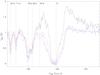 |
Fig. A.1 Superimposed spectra (divided by the continuum) of the ground-state ortho- (black) and para-H |
Low column densities were derived to be on the order of a few 1011 cm-2, except for the 79.5 km s-1component, whose N is several times larger (these values of the column density explain why absorption is not seen for other transitions). From these calculations, we evaluated the o/p ratio for each component. Surprisingly, if the absorption is due to cold foreground clouds, the o/p ratio does not strongly diverge from three when we take the uncertainties into account. This means that, in these clouds, water is produced in what is called the high temperature regime (Tspin > 50 K). We of course stress that the opacities might be underestimated because of the assumptions that we made.
All Tables
Herschel-HIFI observed line transitions in W43-MM1. Frequencies are from Pearson et al. (1991). Beam and ηmb are from Roelfsema et al. (2012). The rms is the noise at the given spectral resolution δν.
Observed line-emission parameters for the detected lines. νLSR is the line peak velocity.
Parameters used in Whitney-Robitaille continuum model and derived physical quantities.
Opacity, total column density, and o/p ratio derived for each line-of-sight absorption component detected.
All Figures
|
Fig. 1 HIFI spectra of H |
| In the text | |
|
Fig. 2 HIFI spectra of H |
| In the text | |
|
Fig. 3 Continuum-subtracted HIFI spectra of the C18O 9–8 and CS 11–10 lines (in black). The model fits are shown as red lines over the spectra. Vertical dotted lines indicate the VLSR at 99.4 km s-1. The spectra have been smoothed to 0.2 km s-1. The unidentified line in absorption seen at 88.6 km s-1 is indicated. |
| In the text | |
|
Fig. 4 Density and temperature profile derived from SED modeling. |
| In the text | |
|
Fig. 5 Spectral energy distribution for W43-MM1 calculated using the Whitney-Robitaille model for the parameters in Table 3. Error bars are from the references cited in Sect. 5.1. |
| In the text | |
|
Fig. 6 Variation in the turbulent and infall velocities, respectively Vturb and Vinf, with the radius R (AU) to the central object. We overplot the radii corresponding to the temperature jump (dashed) in the model and to the radius where lines of different energies originate mainly from the upper energy levels as dashed lines. |
| In the text | |
|
Fig. A.1 Superimposed spectra (divided by the continuum) of the ground-state ortho- (black) and para-H |
| In the text | |
Current usage metrics show cumulative count of Article Views (full-text article views including HTML views, PDF and ePub downloads, according to the available data) and Abstracts Views on Vision4Press platform.
Data correspond to usage on the plateform after 2015. The current usage metrics is available 48-96 hours after online publication and is updated daily on week days.
Initial download of the metrics may take a while.