| Issue |
A&A
Volume 542, June 2012
|
|
|---|---|---|
| Article Number | A32 | |
| Number of page(s) | 11 | |
| Section | Extragalactic astronomy | |
| DOI | https://doi.org/10.1051/0004-6361/201117329 | |
| Published online | 30 May 2012 | |
The Herschel Virgo Cluster Survey
X. The relationship between cold dust and molecular gas content in Virgo spirals⋆
1 Osservatorio Astrofisico di Arcetri – INAF, Largo E. Fermi 5, 50125 Firenze, Italy
e-mail: This email address is being protected from spambots. You need JavaScript enabled to view it.
; This email address is being protected from spambots. You need JavaScript enabled to view it.
; This email address is being protected from spambots. You need JavaScript enabled to view it.
; This email address is being protected from spambots. You need JavaScript enabled to view it.
; This email address is being protected from spambots. You need JavaScript enabled to view it.
;
2 European Southern Observatory, Karl-Schwarzschild-Strasse 2, 85748 Garching bei Munchen, Germany
3 Laboratoire d’Astrophysique de Marseille, UMR 6110 CNRS, 38 rue F. Joliot-Curie, 13388 Marseille, France
4 Jodrell Bank Centre for Astrophysics, Alan Turing Building, School of Physics and Astronomy, University of Manchester, Manchester M13 9PL, UK
5 Department of Physics and Astronomy, Cardiff University, The Parade, Cardiff, CF24 3AA, UK
6 CAAUL, Observatorio Astronomico de Lisboa, Universidade de Lisboa, Tapada de Ajuda, 1349-018 Lisboa, Portugal
7 Service d’Astrophysique, CEA/Saclay, l’Orme des Merisiers, 91191 Gif-sur-Yvette, France
8 Joint ALMA Office, Alonso de Cordova 3107, Vitacura,
and Departamento de Astronomia, Universidad de Chile, Casilla 36-D, Santiago, Chile
9 Sterrenkundig Observatorium, Universiteit Gent, Krijgslaan 281 S9, 9000 Gent, Belgium
Received: 24 May 2011
Accepted: 16 April 2012
Abstract
Aims. We examine whether dust mass can trace the total or molecular gas mass in late-type Virgo cluster galaxies, and how the environment affects the dust-to-gas ratio and the molecular fraction.
Methods. Using the far-infrared emission, as observed by the Herschel Virgo Cluster Survey (HeViCS), and the integrated HI 21-cm and CO J = 1−0 line brightness, we infer the dust and total gas mass for a magnitude limited sample of 35 metal rich spiral galaxies. Environmental disturbances on each galaxy are considered by means of the HI deficiency parameter.
Results. The CO flux correlates tightly and linearly with far-infrared fluxes observed by Herschel, especially with the emission at 160, 250 and 350 μm. Molecules in these galaxies are more closely related to cold dust rather than to dust heated by star formation or to optical/NIR brightness. We show that dust mass establishes a stronger correlation with the total gas mass than with the atomic or molecular component alone. The correlation is non-linear since lower mass galaxies have a lower dust-to-gas ratio. The dust-to-gas ratio increases as the HI deficiency increases, but in highly HI deficient galaxies it stays constant. Dust is in fact less affected than atomic gas by weak cluster interactions, which remove most of the HI gas from outer and high latitudes regions. Highly disturbed galaxies, in a dense cluster environment, can instead loose a considerable fraction of gas and dust from the inner regions of the disk keeping constant the dust-to-gas ratio. There is evidence that the molecular phase is also quenched. This quencing becomes evident by considering the molecular gas mass per unit stellar mass. Its amplitude, if confirmed by future studies, highlights that molecules are missing in Virgo HI deficient spirals, but to a somewhat lesser extent than dust.
Key words: galaxies: clusters: general / galaxies: clusters: individual: Virgo / ISM: molecules / infrared: galaxies / dust, extinction
Herschel is an ESA space observatory with science instruments provided by European-led Principal Investigator consortia and with important participation from NASA.
© ESO, 2012
1. Introduction
Dust and gas in galaxies are essential ingredients for star formation. Stars are born because of the cooling and fragmentation of molecular gas, which in today’s galaxies forms from atomic gas primarily by catalytic reactions on the surface of dust grains (Gould & Salpeter 1963). Dust and atomic gas are, however, only part of the picture because the fractional abundance of molecules depends on a delicate balance between formation and dissociation processes (Hollenbach et al. 1971) and on the self-shielding ability of molecular species from ultraviolet radiation (Draine & Bertoldi 1996). The presence of prominent arms and high interstellar pressure in the disk favour high molecular abundances (Elmegreen 1993). In order to study the relation between dust and molecules it is important to have a good inventory of their masses and distribution in a variety of galaxy types and environments. Intense interstellar radiation fields and galaxy-galaxy interactions or gas stripping as the galaxy moves through inter-cluster gas can quench the growth of molecular clouds through galaxy starvation or strangulation (Larson et al. 1980; Bekki et al. 2002; Boselli & Gavazzi 2006; Fumagalli & Gavazzi 2008; Fumagalli et al. 2009). But there is not a unanimous consent on how environmental conditions affect the molecular component: this is more bounded to the galaxy potential well, being more confined inside the disk, and less disturbed by the environment (Stark et al. 1986; Solomon & Sage 1988; Kenney & Young 1989).
Measuring the total molecular content of a galaxy is a rather difficult task because molecular hydrogen (H2), the most abundant molecular species, is hard to excite, lacks a permanent electric dipole moment and must radiate through a slow quadrupole transition. The ability of molecular hydrogen to form stars, the so called star formation efficiency, can also vary and hence the star formation rate cannot be used as an indicator of molecular mass (Young 1999; Di Matteo et al. 2007; Murray 2011). Molecular surveys rely on the brightness of CO rotational lines and on CO-to-H2 conversion factors, XCO, to derive the molecular hydrogen mass from the CO luminosity. In general this depends on the CO-to-H2 abundance ratio, which is a function of metallicity and on the self-shielding ability of the two molecules, and on the excitation state of the CO molecules. The CO molecule forms almost exclusively in the gas phase and has a lower capability for self-shielding then H2 due to the low abundance of carbon relative to hydrogen (e.g. Glover & Mac Low 2011). However, there are still discrepant results on how XCO varies, for example as a function of the gas metallicity (Wilson 1995; Israel 1997b; Bolatto et al. 2008; Leroy et al. 2011; Shetty et al. 2011). Infrared emission has been used sometime to find possible variations of the CO-to-H2 conversion factor (Knapp et al. 1987; Israel 1997a,b; Leroy et al. 2007; Gratier et al. 2010; Leroy et al. 2011; Magrini et al. 2011) and estimate the molecular content.
The total dust mass of a galaxy can only be determined if dust emission is traced throughout using multi-wavelength observations from the infrared (IR) to the sub-millimeter. Hot dust, in the proximity of star-forming regions, is similar to the tip of an iceberg: prominent but not representative of the total dust mass. The Herschel Space Observatory (Pilbratt et al. 2010; Poglitsch et al. 2010; Griffin et al. 2010), with its two photometric instruments at far infrared wavelengths (PACS, the Photodetector Array Camera Spectrometer with 70, 100, and 160 μm bands and SPIRE, the Spectral and Photometric Imaging Receiver with 250, 350 and 500 μm bands) can observe both sides of the peak (100–200 μm) in the spectral energy distribution of dust in galaxies. The Herschel Virgo Cluster Survey (HeViCS, Davies et al. 2010), an Herschel open time key project, has mapped an area of the nearby Virgo cluster of galaxies, with PACS and SPIRE to investigate the dust content of galaxies of different morphological types and whether intra-cluster dust is present. Recent studies based on Herschel data (Cortese et al. 2010, 2012) have already pointed out that in a dense cluster environment dust can be removed from galaxy disks.
For a sample of bright spiral galaxies in the Virgo cluster, which have been targets of CO observations, we shall examine the correlation between the dust emission and the CO brightness, integrated over the disk, and between dust and gas masses. An important question to address is, for example, whether HI deficient galaxies are also deficient in their global dust and molecular content and how deficiency affects galaxy evolution (Boselli & Gavazzi 2006). The large number of Virgo spiral galaxies, forming stars actively, will let us investigate whether dust mass establishes a better correlation with the molecular gas mass or with the sum of the atomic and molecular gas mass and to pin down possible environmental effects on the dust-to-gas ratio. A large sample of field galaxies would be an ideal reference sample to have, in order to distinguish environmental effects from properties related to the galaxy quiescent evolution. However, the presence of newly acquired cluster members in a young cluster, such as the Virgo Cluster, offers the possibility of using the HI deficiency as indicator of environmental disturbances. By defining the HI deficiency as the difference between the observed HI mass and that expected in an isolated galaxy, Giovanelli & Haynes (1985) have in fact shown that the HI deficiency increses towards the cluster center. This supports the idea that the HI deficiency can trace environmental effects and that galaxies in the same cluster which are not HI deficient can be considered similar to isolated galaxies.
Another open question is whether dust-to-gas ratio can be used as metallicity indicator. If the production of oxygen and carbon are the same and the production, growth and destruction of solid grains does not change from a galaxy to another, we expect the fraction of condensed elements in grains to be proportional to those in the gas phase. Radial analysis of individual galaxies has shown that this is indeed the case (Magrini et al. 2011; Bendo et al. 2010b) and models have been proposed to predict how the dust abundance varies as galaxies evolve in metallicity (Lisenfeld & Ferrara 1998; Hirashita et al. 2002). Draine et al. (2007) found that the dust-to-gas ratio in the central regions does not depend on the galaxy morphological type for galaxies of type Sa to Sd. But a linear scaling between the metallicity and the dust-to-gas ratio is not always found (Boselli et al. 2002), especially when metal abundances are low (Muñoz-Mateos et al. 2009). However, as shown by Galametz et al. (2011), this might result from an inaccurate determination of dust mass due to the lack of data coverage at long infrared wavelengths. Using the wide wavelength coverage of Herschel we investigate whether the dust-to-gas ratio can be used as metallicity indicator for metal rich spirals in Virgo.
We describe the galaxy sample and the database in Sect. 2, the relation of the CO brightness and gas masses with the far-infrared emission and dust masses in Sect. 3. An analysis of possible environmental effects on the dust and gas content, atomic and molecular, is given in Sect. 4. In Sect. 5 we summarize the main results and conclude.
Galaxies in the M and S samples and related quantities.
2. The sample and the data
Our sample is a magnitude-limited sample of galaxies in the Virgo cluster area mapped by HeViCS. The HeViCS covers ≈ 84 sq. deg. of the Virgo cluster, not the whole cluster area (Davies et al. 2010), and the full-depth region observed with both PACS and SPIRE is limited to 55 sq. deg., due to offsets between scans. Galaxies in the Virgo Cluster Catalogue (VCC) (Binggeli et al. 1985) are included in our sample only if they are of morphological type Sab to Sm, are located in the HeViCS fields, their distance is 17 ≤ D ≤ 32 Mpc, and their total magnitude in the B-system, as given in the Third Reference Catalog of Bright Galaxies (de Vaucouleurs et al. 1995), is BT < 13.04. This limiting magnitude ensures that all galaxies in our sample have been observed and detected at 21-cm and in the CO J = 1–0 line. Very few Virgo galaxies fainter than BT = 13.04 have been detected in the CO J = 1–0 line. In the HeViCS area, and for the selected range of morphological type, our sample is 100% complete down to B-mag 13.04. With respect to the 250 μm flux our sample is 100% complete down to F250 = 5 Jy. The significance of correlations between different galaxy properties are assessed using the Pearson linear correlation coefficient, r.
The complete list of 35 galaxies selected in our sample is given in Table 1. In Col. 1 we give the sample code, which indicates the type of CO observations available for estimating the molecular mass. “M” refers to the main sample, which consists of all galaxies in HeViCS that have been fully mapped in the CO J = 1−0 line. “S” refers to the secondary sample: galaxies in HeViCS which have been detected but not fully mapped in CO. The galaxy name, right ascension and declination are given in Cols. 2−4 respectively. The distance to the galaxy in Mpc, the galaxy morphological type and stellar mass are given in Cols. 5−7, respectively. Distances are determined from the average redshift of the individual cluster sub-groups (Gavazzi et al. 1999) and we adopts the morphological classification scheme of the VCC. Nebular oxygen abundances, 12+log(O/H), from the Sloan Sky Digital Survey are shown in Col. 8. In parenthesis the metallicity inferred from the stellar mass using the mass − metallicity relation of Tremonti et al. (2004) and adopting the functional form fit of Kewley & Ellison (2008). The atomic and molecular hydrogen mass are listed in Cols. 9−11, respectively. The two values of the molecular mass,  and
and  , have been derived from the integrated CO brightness using two different values of the CO-to-H2 conversion factor: a uniform constant value of XCO or a metallicity dependent CO-to-H2 conversion factor (as given in more details in Sect. 2.1). In Col. 12 we give the relevant reference for the integrated CO line intensity. In the last column we indicate the number of positions where CO has been detected/observed or whether the galaxy has been fully mapped. If more than one map is available we take the mean CO brightness and list the references joined by a plus sign.
We derive the stellar mass of each galaxy, M∗, using the B − K color and the K-band luminosity, as described in Mannucci et al. (2005). In order to have a uniform set of photometric data, we use the GOLDMINE database1 (Gavazzi et al. 2003) for the Hα, B-, H- and K-band magnitudes (Gavazzi & Boselli 1996), and for the disk geometrical parameters (Nilson 1973). We derive absolute luminosities after correcting for internal extinction according to the prescription given by Gavazzi & Boselli (1996). Corrections for foreground galactic extinction are small (AV ≃ 0.07).
As a metallicity indicator we use the O/H abundance obtained by Tremonti et al. (2004) from the SDSS data. Metallicity has been estimated by fitting at the same time all prominent emission lines ([O II], Hβ, [O III], Hα, [N II], [S II]) with an integrated galaxy spectrum model (Charlot & Longhetti 2001). Not all galaxies in our sample have SDSS spectra with measurable emission lines or appropriate line ratios needed to derive O/H abundances. This is because SDSS narrow slits are generally positioned on the central high surface brightness regions and the presence of some nuclear activity or of a bulge, prevents the authors from probing emission line HII regions in the disk. Galaxies with very weak emission lines or with anomalous line ratios because of nuclear activity have been discarded by Tremonti et al. (2004). Thanks to the analysis of large galaxy samples from the SDSS, the mass − metallicity relation predicts that metallicity scales with stellar mass until the stellar mass is below ~3 × 10¹⁰ M⊙, then it flattens out. Our sample is representative of the mass − metallicity relation: the dispersion of the original dataset around the functional form fit is ≈0.15 dex (Tremonti et al. 2004; Kewley & Ellison 2008), which is consistent with that of our sample. In this paper we shall use the O/H abundance derived from the mass − metallicity relation for all galaxies with known K-band luminosity.
Values of atomic hydrogen mass are taken from the VLA Imaging of Virgo Spirals in Atomic Gas database (VIVA, Chung et al. 2009a), where possible. We correct the HI masses to reflect the galaxy distances used in the present paper if they differ from the value of 17 Mpc adopted in the VIVA survey. Chung et al. (2009a) have found an excellent agreement between single dish fluxes and VIVA fluxes, with no indication that VIVA data is missing any very extended flux. If the galaxy is not in VIVA the GOLDMINE value of the HI mass is used. We will use Mgas to indicate the total hydrogen mass of a galaxy i.e. the sum of the atomic (MHI) and molecular hydrogen mass (MH2) corrected for helium abundance.
2.1. Integrated CO J = 1–0 brightness and molecular mass estimates
Extensive searches for CO emission in Virgo galaxies have been carried out by a number of authors using single dish mm-telescopes. Only 18 galaxies in the HeViCS area have been mapped (M-sample, plotted with filled circles). Some galaxies have been mapped by more than one team using different telescopes. In this case the total CO fluxes are in good agreement and we use the arithmetic mean of the two values. Uncertainties from the original papers have been adopted. We include in the M-sample NGC 4522 which has been mapped in the CO J = 2–1 line and observed at several positions in the CO J = 1−0 to determine the 2–1/1–0 line ratio. We do not include NGC 4299 whose CO map has a low signal to noise and allows a reliable determination of the total CO brightness only within the Hα emission map boundary. There are 17 galaxies with BT < 13.04 which have been detected in the CO J = 1–0 line with one or several pointed observations across the optical disk (S-sample, plotted with open circles). All but one of these have CO J = 1−0 line emission above 3-σ in at least one beam. Only for NGC 4206 the CO J = 1–0 line has been marginally detected, at the 2-σ level. When the CO line brightness has been measured in more than one position we rely on the total CO flux estimated in the original papers. In these cases the total flux is determined via exponential or Gaussian fits to the radial distribution (Stark et al. 1986; Young et al. 1995). If a galaxy has been detected at just one position we determine its total CO flux assuming an exponential radial distribution, centrally peaked, with scalelength λ = 0.2 R25.
The value λ = 0.2 ± 0.1 R25 is the average radial scalelength of the CO flux distribution inferred for the M-sample (mapped galaxies). This is consistent with the exponential scalelengths measured for the CO emission in nearby galaxies mapped in the Heterodyne Receiver Array CO Line Extragalactic Survey (Leroy et al. 2009). We convolve the exponential function, corrected for disk inclination, with the telescope beam, and compare this to the observed flux in order to determine the central brightness and hence the total CO flux. Notice that S-sample galaxies, as well as mapped Virgo galaxies, do not have enhanced CO emission in the center and are very well represented by exponential functions, as shown by Kuno et al. (2007). For HeViCS galaxies in the Kuno et al. (2007) sample the fraction of molecular gas in the inner regions, fin, is only 0.14 on average, for both Seyfert and non-Seyfert galaxies. The dispersion between the total CO flux as measured from the map, and the value derived from the exponential fit with scalelength λ = 0.2 R25 is 0.15 in log units. This is the error which we add in quadrature to the flux measurement error when computing the uncertainties in the total CO brightness of galaxies in the S-sample.
For 6 galaxies in Table 1 we use newly acquired data from observations with the IRAM 30-m telescope (Pappalardo et al., in prep.). Here we give a brief description of the observations. We searched for CO J = 1–0 and J = 2–1 lines in NGC 4189, NGC 4294, NGC 4298, NGC 4299, NGC 4351, NGC 4388, during June 2010 and April 2011. The FWHM beam is 22 arcsec at 115 GHz, the frequency of the J = 1–0 line used in this paper. We observed the sources in position-switching mode, using the EMIR receiver combination E0/E2 and the VESPA and WILMA backend system with a bandwidth of 480 MHz and 4 GHz, respectively. The on-the-fly mapping mode was used for mapped galaxies. Non-mapped galaxies were sampled along the major axis at 22 arcsec spacing. The spectra were smoothed in velocity to 10.5 km s-1 and the data from different backends were averaged resulting in an rms between 7 and 19 mK.
Herschel fluxes in the various bands, dust masses, temperatures and reduced χ2 for the SED fit.
Two values of the molecular hydrogen mass for each galaxy are listed in Cols. 10 and 11 of Table 1. In Col. 10  is derived from the total integrated CO flux using the given distance and a constant CO-to-H2 conversion factor, equal to that found in the solar neighborhood XCO ≃ 2 × 10²⁰ mols. cm-2/(K km s-1) (Strong & Mattox 1996; Dame et al. 2001; Abdo et al. 2010; Shetty et al. 2011). In Col. 11
  is the molecular hydrogen mass for a metallicity dependent CO-to-H2 conversion factor computed as follows. We assume that the metallicity at the galaxy center, Zc, is that given by the mass − metallicity relation (only for VCC975 we do take the SDSS value because of the unknown K-band magnitude) and that there is a radial metallicity gradient similar to that determined by the oxygen abundances in our own galaxy through optical studies (Rudolph et al. 2006). This can be rewritten as:
 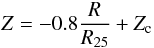 (1)where Z = 12 + log O/H. Using the above equation and the value of the CO-to-H2 conversion factor measured in the solar neighborhood (at R ≃ 0.67 R25) the following radial dependence can be written:
 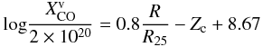 (2)if one assumes a CO-to-H2 conversion factor which varies inversely with metallicity. For Zc = 9.1, a typical value of the central metallicity in our sample, the above equation predicts that the conversion factor is 8 × 1019 cm-2/(K km s-1) at the center and 5 × 1020 cm-2/(K km s-1) at R = R25. Unless stated differently we shall use
  and the corresponding masses (Col. 11 in Table 1) throughout this paper. However, due to the lack of data for radial metallicity gradients in cluster galaxies and to uncertainties of metallicity calibrators, we will quote also results relative to . Given the limited metallicity range of our sample results are not much dependent on the CO-to-H2 factor used (Bolatto et al. 2008; Leroy et al. 2011).
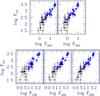 |
Fig. 1 Fluxes in the 5 Herschel bands (in Jy units) versus the total CO J = 1–0 flux (in Jy km s-1). Filled circles are galaxies in the M-sample, open circles galaxies in the S-sample. |
2.2. Far-infrared observations and dust mass estimates
For the far-infrared (FIR) emission we use the HeViCS dataset described in Davies et al. (2012) but with all the eight scans combined, as described in Auld et al. (2012), since Herschel observations have now been completed. The Herschel satellites has scanned the whole area of the survey four times in two orthogonal directions giving a total of eight images for each band. The full width half maximum (FWHM) beam sizes are approximately 9.4 and 13.5 arcsec with pixel sizes of 3.2 and 6.4 arcsec for the 100 and 160 μm PACS channels, respectively. The FWHM of the SPIRE beams are 18.1, 25.2, and 36.9 arcsec with pixel sizes of 6, 8, and 12 arcsec at 250, 350, and 500 μm, respectively.
As shown in Bendo et al. (2010a), emission longward of 100 μm traces the cold dust heated by evolved stars which constitutes the bulk of dust mass in spiral galaxies. We can derive dust masses and temperatures using the PACS and SPIRE fluxes after fitting the spectral energy distribution (SED) between 100 and 500 μm. In Table 2 we show the Herschel fluxes, dust masses and temperatures, and the χ2 values for the SED fits relative to all galaxies in our sample. Dots indicate that the galaxy is outside the area mapped by HeViCS in that band. The errors quoted in Table 2 cover uncertainties due to the choice of the aperture, to the calibration and to photometric random errors (Auld et al. 2012). Calibration uncertainties are the largest errors also for PACS photometry (in this case they have been assumed to be of order of 20%). For bright galaxies, such as those in our sample, the procedure and dataset described in Auld et al. (2012) gives fluxes, dust temperatures and masses which are consistent with those obtained by Davies et al. (2012) using only two orthogonal scans i.e. one quarter of the final exposure times. Using the complete HeViCS dataset we detect all galaxies in all 5 bands. For only one galaxy, NGC 4571, we cannot measure PACS fluxes because it lies outside the boundaries of the PACS mapped area.
The SED fits were done for each galaxy after convolving the modified blackbody model with the spectral response function for each band, thus automatically taking into account color corrections for the specific SED of each object. We used a power law dust emissivity κλ = κ0(λ0/λ)β, with spectral index β = 2 and emissivity κ0 = 0.192 m2 kg-1 at λ0 = 350 μm. These values reproduce the average emissivity of models of the Milky Way dust in the FIR-submm (Draine 2003). They are also consistent with the dust spectral emissivity index β determined in molecular clouds using the recent Planck data (e.g. Planck Collaboration 2011, and references therein). The standard χ2 minimization technique is used in order to derive the dust temperature and mass. Uncertainties in the temperature determination, considering the photometry errors, are about 1–2 K. Uncertainties on dust temperature and mass are only slightly larger for the NGC 4571 for which there is no PACS data. More details on SED fitting are given in Smith et al. (2010); Magrini et al. (2011); Davies et al. (2012). Note that single black body SED models fit well S-sample galaxies as well as M-sample galaxies. All SED fits are displayed by Davies et al. (2012) and by Auld et al. (2012). A two component fit is not well constrained by just five data points in the SED and it would require shorter and longer wavelength data.
3. The correlations between dust and the molecular or total gas mass
Far-infrared fluxes for galaxies in the M-sample correlate well with the total CO flux, as shown in Fig. 1. Pearson linear correlation coefficients r in the log FFIR–log FCO plane are high for fluxes in all 5 Herschel bands, ranging between 0.88 and 0.93 for the whole sample, and between 0.94 and 0.96 for galaxies in the M-sample (the highest being for F160 and F250). Slopes are of order unity (0.92 ± 0.08, 1.04 ± 0.08, 1.08 ± 0.08, 1.10 ± 0.07, 1.09 ± 0.05 for FIR wavelengths from 100 to 500 μm), meaning that the correlation is close to linear. The best linear fit in the logF250–logFCO plane gives for example logFCO = 1.08( ± 0.08)logF250 + 1.45( ± 0.08). These slopes are compatible with those derived considering only galaxies in the M-sample (1.04 ± 0.13, 1.06 ± 0.11, 1.04 ± 0.10, 1.04 ± 0.08, 1.04 ± 0.05 for FIR wavelengths from 100 to 500 μm). The less tight relation between the CO line intensity and hot dust emission in Virgo spirals (e.g. Stark et al. 1986, for IRAS data) suggests that molecules are more closely related to cold dust rather than to dust heated by star formation.
The larger scatter and the slightly lower correlation coefficients found when we include in the analysis galaxies in the S-sample, might be driven by the higher uncertainties on the total CO emission, because of the lack of CO maps. In order to check whether this is indeed the case, or whether a break in the correlation occurs at low luminosities, additional CO maps are needed for galaxies as dim as 13–14 mag in the B-band. To avoid the uncertainties on the integrated CO fluxes for non mapped galaxies we have checked the slope and the scatter of the FIR-CO correlation for galaxy central regions. We convolved the 250 μm maps from the original resolution (FWHM = 18.2′′) to the resolution of pointed CO J = 1–0 observations (which can be found in references to Table 1). At the optical center of galaxies we measure the 250 μm flux in an area as large as the FWHM of the telescope used to measure the CO J = 1–0 line intensity (ranging between 45 and 100 arcsec). Figure 2 shows the resulting correlation between F250 and the CO flux in the same area, as given in the original papers. The straight line, of slope 1.11 ± 0.02, shows the best linear fit to these data. This is compatible with the slope measured when values integrated over the galaxy disk are considered (1.04 ± 0.08). The scatter in the correlation is not reduced with respect to that found for the same quantities integrated over the whole disk.
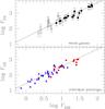 |
Fig. 2 Lower panel: the CO J = 1–0 flux, in Jy km s-1, measured in one beam at the galaxy center, versus the 250 μm flux in Jy in the same area for galaxies in the M- and S-sample. The filled squares (red in the online version) are for beams of 100 arcsec FWHM, while the filled triangles (blue) are for beams of 45–55 arcsec FWHM. Upper panel: same quantities as in the lower panel but integrated over the whole galaxy. Filled circles are for galaxies mapped in CO while open circles are for galaxies whose total integrated CO flux has been inferred using pointed observations (see text for details). |
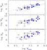 |
Fig. 3 The relation between dust and gaseous masses (HI, H |

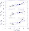 |
Fig. 4 The relation between dust and gaseous masses (in solar mass units) for galaxies with def(HI) > 0.5. Filled and open circles are for galaxies in the M-sample, and S-sample, respectively. The dashed line in the upper panel is the best-fit linear relation for the data shown. |
Dust masses take into account temperature variations which individual FIR fluxes do not. The bluest galaxies have lower dust temperatures i.e a low F250-to-F500 flux ratio. In Fig. 3 we compare the dust mass, Mdust, to the molecular, MH2, atomic, MHI, and total gas mass, Mgas. The lowest scatter in the dust-to-molecular gas mass relation is found if  , for the whole sample (r = 0.81) or for the M-sample alone (r = 0.88 in this case). The correlation for the whole sample reads:
  (3)A flatter, but still compatible slope is obtained if one considers the correlation Mdust–:
  (4)The slope is closer to unity if we consider only galaxies of the M-sample, likely because this sample is more uniform in galaxy morphology (mostly Sc). The best correlation with the dust mass is found for the total gas mass, with a Pearson linear correlation coefficient of 0.91 for the M-sample and of 0.84 for the whole sample. In the last case the best-fit linear relation between Mdust and Mgas reads:
  (5)which implies a lower dust-to-gas ratio for galaxies with a lower gas content. If replaces in the computation of Mgas the slope is 0.85 ± 0.08 and r = 0.88. The decrease of the dust-to-gas ratio, as the gas mass decreases, is not due to the environment: large galaxies, with a large gas mass, are not more HI deficient than small galaxies (with a small gas mass). In Fig. 4 we show the relation between dust and gas mass for HI deficient galaxies with def(HI) > 0.5. The slope of the dust-to-total gas mass relation is 0.76 ± 0.08, compatible with that found for the whole sample or for non-HI deficient galaxies (0.62 ± 0.11). As expected, the dispersion in the Mdust–MHI relation decreases for HI deficient galaxies, which have dispersed the outer gas in the intercluster medium (bottom panel of Fig. 4). In the mass range covered by our sample, environmental effects on the dust-to-gas ratio (see next section) do not depend on galaxy mass. Variations in the dust-to-gas ratio with the global gas content are instead due to internal evolution. Smaller galaxies in the S-sample have on average a higher HI content: they have been unable to increase the dust abundance and to convert much of their atomic gas into molecular gas due also to their extended outer HI disks. As shown by Pappalardo et al. (in prep.) in a spatially resolved study, the relation between dust emission and gas surface density in the inner regions is very tight, with a slope closer to one for metal rich galaxies.
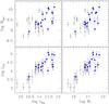 |
Fig. 5 The relations between the extinction corrected Hα luminosity and stellar mass and the CO luminosity or total gas mass. Luminosities and masses are in solar luminosity and mass units, respectively. Symbols for galaxies in different samples are coded as in Fig. 1. |
In the following we convert the flux density in an Herschel band, Fν, into luminosity Lν = 4πD2νFν and express Lν in solar units. Hence we convert the CO J = 1–0 total flux in Jy km s-1 into LCO in solar units by multiplying FCO by 0.12  . The 250 μm luminosity, similar to Mdust, correlates better with the total gas mass rather than with the HI or H2 mass alone.
The scatter in the LCO–LB,H,K,Hα relation, the B, H, K-band and Hα luminosities, which we corrected for internal extinction, is larger than observed between LCO and the luminosities in the various Herschel bands. We display LCO versus LHα and M ∗ in Fig. 5 and below we give the relations between LCO and LB, LHα, M ∗ , L250 for the whole sample (in solar units): ![Mathematical equation: \begin{eqnarray} {\hbox {log }L}_{\rm CO} &=& 1.10 \times {\hbox{log }L}_B -6.7 \qquad r = 0.78 \\[3.5mm] {\hbox {log }L}_{\rm CO} &=& 0.87 \times {\hbox{log }L}_{{\rm H}\alpha} -5.4 \qquad r = 0.83 \\[3.5mm] {\hbox{log }L}_{\rm CO} &=& 0.78 \times {\hbox{log }M}_* -4.3 \qquad r = 0.85 \\[3.5mm] {\hbox{log }L}_{\rm CO} &=& 1.07 \times {\hbox{log }L}_{250} -5.6 \qquad r = 0.92. \label{eq:250h2} \end{eqnarray}](/articles/aa/full_html/2012/06/aa17329-11/aa17329-11-eq100.png) The correlations of Mgas with LHα or M ∗ are also less tight (see Fig. 5) than with L250 and much weaker correlations are found for MHI. This confirms that the main correlation with the CO J = 1–0 line intensity is indeed established by the cold dust emission. In our sample, which spans a limited metallicity range, the CO J = 1–0 line emission traces molecular hydrogen which forms on dust, and this explains the correlation. Star formation is not ubiquitous in molecular clouds and, as a result, a less tight correlation of the CO J = 1–0 line emission with Hα luminosity is observed.
The correlations of Mgas with LHα or M ∗ are also less tight (see Fig. 5) than with L250 and much weaker correlations are found for MHI. This confirms that the main correlation with the CO J = 1–0 line intensity is indeed established by the cold dust emission. In our sample, which spans a limited metallicity range, the CO J = 1–0 line emission traces molecular hydrogen which forms on dust, and this explains the correlation. Star formation is not ubiquitous in molecular clouds and, as a result, a less tight correlation of the CO J = 1–0 line emission with Hα luminosity is observed.
4. Environmental effects on the dust and gas content
One aspect related to the environment which we are going to address is whether the global dust-to-gas ratio can be used as a metallicity indicator for cluster galaxies. We devote the rest of this section to investigate if the environment can enhance or inhibit the persistence of dust and molecules in galaxies (Stark et al. 1986; Fumagalli & Gavazzi 2008). The environmental effects are examined primarily in terms of HI deficiency which we have computed for all galaxies in our sample following the prescription of Haynes & Giovanelli (1984).
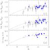 |
Fig. 6 In panel a) the mass − metallicity relation derived by Tremonti et al. (2004) (dashed line) is plotted together with data for galaxies in our sample with a known SDSS metallicity, given in Table 1. In panels b) and c) the mass − metallicity relation has been scaled so that its peak reproduces the average dust-to-gas ratio for the M-sample. In panel b) |
In Fig. 6a we show the consistency of the metallicities of the central regions of galaxies in our sample with the mass − metallicity relation. In Fig. 6b the dust-to-gas ratio is plotted as a function of stellar mass. The dashed line shows the mass − metallicity relation scaled so that its peak reproduces the average dust-to-gas ratio found for the M-sample, i.e. − 1.9 ± 0.15 in log. This implies a dust-to-gas ratio of 0.013, a factor 1.8 higher than the value of 0.007 found for the Milky Way (Draine et al. 2007), whose central regions have metal abundances comparable to those of the M-sample, but only slightly higher that the theoretical value of 0.01 (Draine et al. 2007). In panel c we show the better agreement with the mass − metallicity relation if is used instead (i.e. a constant CO-to-H2 conversion factor). In this case the discrepancy between the average dust-to-gas ratio in the Milky Way and that of the M-sample is reduced.
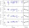 |
Fig. 7 The dust-to-gas ratio, dust-to-stellar mass ratio, molecular-to-stellar mass ratio and the molecular fraction as a function of the HI deficiency. Panels to the left show the data with symbols as in previous figures: filled circles are galaxies in the M-sample, open circles are galaxies in the S-sample. Continuous lines in each panel are best fits to linear relation between def(HI) and the variable shown on the y-axis. Panels to the right of the figure show mean values in three HI deficiency bins. |
Galaxies in the S-sample lie mostly below the mass − metallicity relation both in panels b and c. For galaxies in the S-sample the dust-to-gas ratio is lower than what a linear scaling with the metallicity would predict, similar to what Muñoz-Mateos et al. (2009) find. These results holds even if we consider HI deficient and non-HI deficient galaxies separately. Likely, this is a consequence that metal abundances and dust-to-gas ratios sample different galaxy regions. The SDSS survey measures metal abundances at the galaxy center while the dust-to-gas ratio in this paper is a quantity integrated over the whole disk. Unenriched extended gaseous disks are more pronounced in low mass blue galaxies. The average dust-to-gas ratio for the M- and S-sample together is −2.1 ± 0.3 in log. The best linear fit to the M- and S-sample data for Md/Mgas as a function of M∗ reads:  (10)This relation (with correlation coefficient r = 0.65) is shown by the dot-dashed line in Fig. 6b.
To check whether the HI deficiency affects the dust-to-gas ratio we show this last variable as a function of the HI deficiency, def(HI), in the bottom panel of Fig. 7. We can see that as the HI deficiency increases, the dust-to-gas ratio increases but the correlation is weak (best fit slope is 0.26 ± 0.06, r = 0.58). This trend can be due to two possible effects: the first one is gas removal which affects the dust content less because dust lies more deeply in the potential well of the galaxy. The second one is an evolutionary effect: if the galaxy entering the cluster turns off gas infall, it uses its gas reservoir to make more metals and stars. If this were the dominant effect, galaxies with higher metallicity (with respect to the metallicities predicted by the mass − metallicity relation) should be more HI deficient. We do not find any correlation between the HI deficiency and the scatter in metallicity with respect to the mass − metallicity relation. Hence, gas removal is responsible for the observed trend. The small panels on the right side of Fig. 7 show the average values in 3 def(HI) bins. It is important to note that the dust-to-gas mass ratio does not increase as the galaxy becomes highly HI deficient, while between non-HI deficient galaxies and galaxies which have a mild deficiency this ratio increases by a factor two. This finding suggests that when the galaxy is highly disturbed the galaxy also becomes dust deficient. In terms of total mass, a small disturbance mostly affects the outer HI envelope and does not much affect the total dust mass since dust is more segregated in the inner regions of the disk (both in height and radially). A similar conclusion has been reached by Cortese et al. (2012) by comparing a sample of field and cluster spirals. They find that the effect of dust removal from the star-forming disk of cluster galaxies is less strong than what is observed for the atomic gas.
To investigate further whether some fraction of dust mass is lost as the galaxy moves through the cluster, we normalize the dust mass to the stellar mass. Dust removal is responsible for the correlation between the dust-to-stellar mass ratio and the HI deficiency shown in Fig. 7b. Galaxies with a higher HI deficiency have a lower dust-to-stellar mass ratio, only 25% of that observed in non HI-deficient galaxies. The slope of the correlation is −0.48 ± 0.08 and the Pearson linear correlation coefficient is −0.72. Dust deficiency in HI deficient Virgo spirals has been pointed out already by Cortese et al. (2010) in a spatially resolved study. The authors show that the extent of the dust disk is significantly reduced in HI truncated disk, due to stripping by the cluster environment There is the possibility that dust removal could be more effective in low-metallicity, low-mass galaxies with shallow potential wells (Boselli & Gavazzi 2006; Bendo et al. 2007) but the HI deficiency does not show any dependence on the stellar mass.
To analyze possible environmental effects on the molecular component we use the MH2-to-M∗ and MH2-to-Mgas ratios. We show these as a function of def(HI) in the top panels of Fig. 7. The best fitting linear relation between log MH2/M∗ and def(HI) has a slope of −0.35 ± 0.11. The dependence on the HI deficiency of ratios involving the molecular mass, or the CO luminosity, is weaker (r ~ 0.5) than for the dust component. If confirmed by future data this correlation implies that HI deficient galaxies are also H2 deficient due to molecular gas removal or to quenching of molecule formation in perturbed gas. For our sample the MH2/M∗–def(HI) relation does not dependent on XCO: the slope of the correlation between the LCO-to-M∗ ratio and the HI deficiency is also shallow (−0.28 ± 0.09) and consistent with that found for the MH2-to-M∗ ratio. The gas molecular fraction, MH2/Mgas, increases as the HI deficiency increases (Fig. 7d) because the atomic gas mass is more heavily removed in the cluster environment.
As shown in Fig. 7c, highly HI deficient galaxies can quench or remove as much as 50–60% of their original molecular content. If we consider only the mapped galaxies in the M-sample the decrease of H2 content is confirmed and becomes more extreme since the CO luminosity, as well as the H2 mass, shows a steeper decrease with the HI deficiency parameter. A future comparison with a field galaxy sample is desirable to confirm this finding. The cluster environment strips out part of the tenuous atomic ISM (e.g. outer disks and high latitude gas) more easily than dust and H2 gas, which is more confined to the mid-plane and to the inner star forming disk. In terms of total mass, dust and molecules are less affected by the environment than the HI gas. Highly disturbed galaxies have considerably lower dust content than their quiescent counterparts and higher molecular fractions.
Figure 8 shows possible dependencies of galaxy properties on the distance from the cluster center. Non-HI deficient galaxies avoid the cluster center, where a higher fraction of Sab and Sb (open triangles) can be found. The dispersion across the whole cluster is large because we are using projected distances. The evidence that dust deficient galaxies and galaxies with a lower LCO/M∗ are located in projection near the cluster center is marginal (see bottom and top panels of Fig. 8).
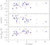 |
Fig. 8 The dust-stellar mass ratio, the HI deficiency and the ratio between the CO luminosity and the stellar mass are shown as a function of the projected distance from the Virgo cluster center. Galaxies are coded as in Fig. 1. The open (red) triangles indicate galaxies of morphological type Sab or Sb. |
5. Summary
The relations between dust and gaseous masses have been examined in this paper for a magnitude limited sample of late type Virgo Cluster galaxies in the HeViCS fields. The Herschel Space Observatory has detected cold dust emission for all galaxies in our sample with the PACS and SPIRE detector at 100, 160, 250, 350 and 500 μm. We summarize below the main results:
-
There is a tight correlation between the total CO J = 1–0 flux and the cold dust emission. Molecules are more closely related to cold dust rather than to dust heated by star formation or to other galaxy integrated quantities such as blue luminosity, star formation or stellar mass.
-
Dust mass correlates better with the total (atomic+ molecular) gas mass rather than with the atomic or molecular gas alone. Infrared-dim galaxies are unable to convert much of their atomic gas into molecular gas. Galaxies with a low molecular-to-total gas ratios have lower dust temperatures, are intrinsically faint and blue and a have a high gas-to-stellar mass ratios.
-
The dust-to-gas mass ratio typically decreases as the galaxy stellar mass decreases, faster than predicted by the mass − metallicity relation. We find a population of galaxies with a lower dust-to-gas ratio than what a linear scaling with metallicity would imply. Likely this is because the total gas mass of a galaxy includes the unenriched extended disk. In fact these galaxies are HI rich with a less prominent stellar mass.
-
Galaxies with a mild HI-deficiency have a higher dust-to-gas ratios than non HI-deficient galaxies. This implies a higher efficiency of the cluster stripping process on the HI gas rather than on the dust, which is more confined inside the disk. However, the cluster environment is able to remove some dust from the galaxy disk as well. The dust mass per unit stellar mass decreases as the HI deficiency increases, and highly HI deficient galaxies can have up to 75% less dust than non HI deficient galaxies.
-
There is evidence of molecular hydrogen quenching or stripping in HI deficient galaxies. This evidence is found by considering the molecular gas per unit stellar mass. If its amplitude is confirmed by future data implies that molecules are missing in Virgo HI deficient spirals, but to a somewhat lesser extent than dust. The molecular fraction increases as the HI deficiency increases because the cluster environment affects molecules to a lesser extent than atomic gas.
-
Our results have been confirmed using various assumptions on the CO-to-H2 conversion factor. We cannot constrain possible dependencies of XCO from galaxy properties, such as the disk morphology or metallicity, due to the limited dynamical range of these parameters in the sample examined.
Acknowledgments
The recent IRAM observations presented in this paper have benefited from research funding from the European Community’s Seventh Framework Programme. The research leading to these results has received funding from the Agenzia Spaziale Italiana (ASI-INAF agreements I/016/07/0 and I/009/10/0) and from the European Community’s Seventh Framework Programme (/FP7/2007-2013/ under grant agreement No. 229517). C.V. received support from the ALMA-CONICYT Fund for the Development of Chilean Astronomy (Project 31090013) and from the Center of Excellence in Astrophysics and Associated Technologies (PBF06).
References
- Abdo, A. A., Ackermann, M., Ajello, M., et al. 2010, ApJ, 710, 133 [NASA ADS] [CrossRef] [Google Scholar]
- Auld, R., et al. 2012, MNRAS, submitted [Google Scholar]
- Bekki, K., Couch, W. J., & Shioya, Y. 2002, ApJ, 577, 651 [NASA ADS] [CrossRef] [Google Scholar]
- Bendo, G. J., Calzetti, D., Engelbracht, C. W., et al. 2007, MNRAS, 380, 1313 [NASA ADS] [CrossRef] [Google Scholar]
- Bendo, G. J., Wilson, C. D., Pohlen, M., et al. 2010a, A&A, 518, L65 [NASA ADS] [CrossRef] [EDP Sciences] [Google Scholar]
- Bendo, G. J., Wilson, C. D., Warren, B. E., et al. 2010b, MNRAS, 402, 1409 [NASA ADS] [CrossRef] [Google Scholar]
- Binggeli, B., Sandage, A., & Tammann, G. A. 1985, AJ, 90, 1681 [NASA ADS] [CrossRef] [Google Scholar]
- Bolatto, A. D., Leroy, A. K., Rosolowsky, E., Walter, F., & Blitz, L. 2008, ApJ, 686, 948 [NASA ADS] [CrossRef] [Google Scholar]
- Boselli, A., & Gavazzi, G. 2006, PASP, 118, 517 [NASA ADS] [CrossRef] [Google Scholar]
- Boselli, A., Casoli, F., & Lequeux, J. 1995, A&AS, 110, 521 [NASA ADS] [Google Scholar]
- Boselli, A., Lequeux, J., & Gavazzi, G. 2002, A&A, 384, 33 [NASA ADS] [CrossRef] [EDP Sciences] [Google Scholar]
- Charlot, S., & Longhetti, M. 2001, MNRAS, 323, 887 [NASA ADS] [CrossRef] [Google Scholar]
- Chung, A., van Gorkom, J. H., Kenney, J. D. P., Crowl, H., & Vollmer, B. 2009a, AJ, 138, 1741 [NASA ADS] [CrossRef] [Google Scholar]
- Chung, E. J., Rhee, M., Kim, H., et al. 2009b, ApJS, 184, 199 [NASA ADS] [CrossRef] [Google Scholar]
- Cortese, L., Davies, J. I., Pohlen, M., et al. 2010, A&A, 518, L49 [NASA ADS] [CrossRef] [EDP Sciences] [Google Scholar]
- Cortese, L., Ciesla, L., Boselli, A., et al. 2012, A&A, 540, A52 [NASA ADS] [CrossRef] [EDP Sciences] [Google Scholar]
- Dame, T. M., Hartmann, D., & Thaddeus, P. 2001, ApJ, 547, 792 [NASA ADS] [CrossRef] [Google Scholar]
- Davies, J. I., Baes, M., Bendo, G. J., et al. 2010, A&A, 518, L48 [NASA ADS] [CrossRef] [EDP Sciences] [Google Scholar]
- Davies, J. I., Bianchi, S., Cortese, L., et al. 2012, MNRAS, 419, 3505 [NASA ADS] [CrossRef] [Google Scholar]
- de Vaucouleurs, G., de Vaucouleurs, A., Corwin, H. G., et al. 1995, VizieR Online Data Catalog, 7155 [Google Scholar]
- Di Matteo, P., Combes, F., Melchior, A., & Semelin, B. 2007, A&A, 468, 61 [NASA ADS] [CrossRef] [EDP Sciences] [Google Scholar]
- Draine, B. T. 2003, ARA&A, 41, 241 [NASA ADS] [CrossRef] [Google Scholar]
- Draine, B. T., & Bertoldi, F. 1996, ApJ, 468, 269 [NASA ADS] [CrossRef] [EDP Sciences] [Google Scholar]
- Draine, B. T., Dale, D. A., Bendo, G., et al. 2007, ApJ, 663, 866 [NASA ADS] [CrossRef] [Google Scholar]
- Elmegreen, B. G. 1993, ApJ, 411, 170 [NASA ADS] [CrossRef] [Google Scholar]
- Fumagalli, M., & Gavazzi, G. 2008, A&A, 490, 571 [NASA ADS] [CrossRef] [EDP Sciences] [Google Scholar]
- Fumagalli, M., Krumholz, M. R., Prochaska, J. X., Gavazzi, G., & Boselli, A. 2009, ApJ, 697, 1811 [NASA ADS] [CrossRef] [Google Scholar]
- Galametz, M., Madden, S. C., Galliano, F., et al. 2011, A&A, 532, A56 [NASA ADS] [CrossRef] [EDP Sciences] [Google Scholar]
- Gavazzi, G., & Boselli, A. 1996, Astrophys. Lett. Comm., 35, 1 [Google Scholar]
- Gavazzi, G., Boselli, A., Scodeggio, M., Pierini, D., & Belsole, E. 1999, MNRAS, 304, 595 [NASA ADS] [CrossRef] [Google Scholar]
- Gavazzi, G., Boselli, A., Donati, A., Franzetti, P., & Scodeggio, M. 2003, A&A, 400, 451 [NASA ADS] [CrossRef] [EDP Sciences] [Google Scholar]
- Giovanelli, R., & Haynes, M. P. 1985, ApJ, 292, 404 [CrossRef] [Google Scholar]
- Glover, S. C. O., & Mac Low, M. 2011, MNRAS, 412, 337 [NASA ADS] [CrossRef] [MathSciNet] [Google Scholar]
- Gould, R. J., & Salpeter, E. E. 1963, ApJ, 138, 393 [NASA ADS] [CrossRef] [Google Scholar]
- Gratier, P., Braine, J., Rodriguez-Fernandez, N. J., et al. 2010, A&A, 512, A68 [NASA ADS] [CrossRef] [EDP Sciences] [Google Scholar]
- Griffin, M. J., Abergel, A., Abreu, A., et al. 2010, A&A, 518, L3 [Google Scholar]
- Haynes, M. P., & Giovanelli, R. 1984, AJ, 89, 758 [NASA ADS] [CrossRef] [Google Scholar]
- Hirashita, H., Tajiri, Y. Y., & Kamaya, H. 2002, A&A, 388, 439 [NASA ADS] [CrossRef] [EDP Sciences] [Google Scholar]
- Hollenbach, D. J., Werner, M. W., & Salpeter, E. E. 1971, ApJ, 163, 165 [NASA ADS] [CrossRef] [Google Scholar]
- Israel, F. P. 1997a, A&A, 317, 65 [NASA ADS] [Google Scholar]
- Israel, F. P. 1997b, A&A, 328, 471 [NASA ADS] [Google Scholar]
- Kenney, J. D. P., & Young, J. S. 1989, ApJ, 344, 171 [NASA ADS] [CrossRef] [Google Scholar]
- Kewley, L. J., & Ellison, S. L. 2008, ApJ, 681, 1183 [NASA ADS] [CrossRef] [Google Scholar]
- Knapp, G. R., Helou, G., & Stark, A. A. 1987, AJ, 94, 54 [NASA ADS] [CrossRef] [Google Scholar]
- Kuno, N., Sato, N., Nakanishi, H., et al. 2007, PASJ, 59, 117 [NASA ADS] [Google Scholar]
- Larson, R. B., Tinsley, B. M., & Caldwell, C. N. 1980, ApJ, 237, 692 [NASA ADS] [CrossRef] [Google Scholar]
- Leroy, A., Bolatto, A., Stanimirovic, S., et al. 2007, ApJ, 658, 1027 [NASA ADS] [CrossRef] [Google Scholar]
- Leroy, A. K., Walter, F., Bigiel, F., et al. 2009, AJ, 137, 4670 [NASA ADS] [CrossRef] [Google Scholar]
- Leroy, A. K., Bolatto, A., Gordon, K., et al. 2011, ApJ, 737, 12 [NASA ADS] [CrossRef] [Google Scholar]
- Lisenfeld, U., & Ferrara, A. 1998, ApJ, 496, 145 [NASA ADS] [CrossRef] [Google Scholar]
- Magrini, L., Bianchi, S., Corbelli, E., et al. 2011, A&A, 535, A13 [NASA ADS] [CrossRef] [EDP Sciences] [Google Scholar]
- Mannucci, F., Della Valle, M., Panagia, N., et al. 2005, A&A, 433, 807 [NASA ADS] [CrossRef] [EDP Sciences] [Google Scholar]
- Muñoz-Mateos, J. C., Gil de Paz, A., Boissier, S., et al. 2009, ApJ, 701, 1965 [NASA ADS] [CrossRef] [Google Scholar]
- Murray, N. 2011, ApJ, 729, 133 [NASA ADS] [CrossRef] [Google Scholar]
- Nilson, P. 1973, Uppsala general catalogue of galaxies (Uppsala: Astronomiska Observatorium) [Google Scholar]
- Pilbratt, G. L., Riedinger, J. R., Passvogel, T., et al. 2010, A&A, 518, L1 [CrossRef] [EDP Sciences] [Google Scholar]
- Planck Collaboration, Abergel, A., Ade, P. A. R., et al. 2011, A&A, 536, A25 [NASA ADS] [CrossRef] [EDP Sciences] [Google Scholar]
- Poglitsch, A., Waelkens, C., Geis, N., et al. 2010, A&A, 518, L2 [NASA ADS] [CrossRef] [EDP Sciences] [Google Scholar]
- Rudolph, A. L., Fich, M., Bell, G. R., et al. 2006, ApJS, 162, 346 [NASA ADS] [CrossRef] [Google Scholar]
- Shetty, R., Glover, S. C., Dullemond, C. P., et al. 2011, MNRAS, 415, 3253 [NASA ADS] [CrossRef] [Google Scholar]
- Smith, M. W. L., Vlahakis, C., Baes, M., et al. 2010, A&A, 518, L51 [NASA ADS] [CrossRef] [EDP Sciences] [Google Scholar]
- Solomon, P. M., & Sage, L. J. 1988, ApJ, 334, 613 [NASA ADS] [CrossRef] [Google Scholar]
- Stark, A. A., Knapp, G. R., Bally, J., et al. 1986, ApJ, 310, 660 [NASA ADS] [CrossRef] [Google Scholar]
- Strong, A. W., & Mattox, J. R. 1996, A&A, 308, L21 [NASA ADS] [Google Scholar]
- Tremonti, C. A., Heckman, T. M., Kauffmann, G., et al. 2004, ApJ, 613, 898 [NASA ADS] [CrossRef] [Google Scholar]
- Vollmer, B., Braine, J., Pappalardo, C., & Hily-Blant, P. 2008, A&A, 491, 455 [NASA ADS] [CrossRef] [EDP Sciences] [Google Scholar]
- Wilson, C. D. 1995, ApJ, 448, L97 [NASA ADS] [CrossRef] [Google Scholar]
- Young, J. S. 1999, ApJ, 514, L87 [NASA ADS] [CrossRef] [Google Scholar]
- Young, J. S., Xie, S., Tacconi, L., et al. 1995, ApJS, 98, 219 [NASA ADS] [CrossRef] [Google Scholar]
All Tables
Herschel fluxes in the various bands, dust masses, temperatures and reduced χ2 for the SED fit.
All Figures
|
Fig. 1 Fluxes in the 5 Herschel bands (in Jy units) versus the total CO J = 1–0 flux (in Jy km s-1). Filled circles are galaxies in the M-sample, open circles galaxies in the S-sample. |
| In the text | |
|
Fig. 2 Lower panel: the CO J = 1–0 flux, in Jy km s-1, measured in one beam at the galaxy center, versus the 250 μm flux in Jy in the same area for galaxies in the M- and S-sample. The filled squares (red in the online version) are for beams of 100 arcsec FWHM, while the filled triangles (blue) are for beams of 45–55 arcsec FWHM. Upper panel: same quantities as in the lower panel but integrated over the whole galaxy. Filled circles are for galaxies mapped in CO while open circles are for galaxies whose total integrated CO flux has been inferred using pointed observations (see text for details). |
| In the text | |
|
Fig. 3 The relation between dust and gaseous masses (HI, H |
| In the text | |
|
Fig. 4 The relation between dust and gaseous masses (in solar mass units) for galaxies with def(HI) > 0.5. Filled and open circles are for galaxies in the M-sample, and S-sample, respectively. The dashed line in the upper panel is the best-fit linear relation for the data shown. |
| In the text | |
|
Fig. 5 The relations between the extinction corrected Hα luminosity and stellar mass and the CO luminosity or total gas mass. Luminosities and masses are in solar luminosity and mass units, respectively. Symbols for galaxies in different samples are coded as in Fig. 1. |
| In the text | |
|
Fig. 6 In panel a) the mass − metallicity relation derived by Tremonti et al. (2004) (dashed line) is plotted together with data for galaxies in our sample with a known SDSS metallicity, given in Table 1. In panels b) and c) the mass − metallicity relation has been scaled so that its peak reproduces the average dust-to-gas ratio for the M-sample. In panel b) |
| In the text | |
|
Fig. 7 The dust-to-gas ratio, dust-to-stellar mass ratio, molecular-to-stellar mass ratio and the molecular fraction as a function of the HI deficiency. Panels to the left show the data with symbols as in previous figures: filled circles are galaxies in the M-sample, open circles are galaxies in the S-sample. Continuous lines in each panel are best fits to linear relation between def(HI) and the variable shown on the y-axis. Panels to the right of the figure show mean values in three HI deficiency bins. |
| In the text | |
|
Fig. 8 The dust-stellar mass ratio, the HI deficiency and the ratio between the CO luminosity and the stellar mass are shown as a function of the projected distance from the Virgo cluster center. Galaxies are coded as in Fig. 1. The open (red) triangles indicate galaxies of morphological type Sab or Sb. |
| In the text | |
Current usage metrics show cumulative count of Article Views (full-text article views including HTML views, PDF and ePub downloads, according to the available data) and Abstracts Views on Vision4Press platform.
Data correspond to usage on the plateform after 2015. The current usage metrics is available 48-96 hours after online publication and is updated daily on week days.
Initial download of the metrics may take a while.