© ESO, 2012

1. Introduction

Hot massive stars lose mass via stellar winds. Mass loss plays an important role in the stellar evolution and strongly affects the interstellar environment (Bresolin et al. 2008). To better understand the evolution of hot massive stars and their influence on the environment, it is necessary to determine their mass-loss rates reliably. Many sophisticated models of the stellar evolution have been calculated (see Maeder & Meynet 2010, for a review). However, these evolutionary tracks depend sensitively on the adopted mass-loss rates, which are still far from being empirically established.

Since the 1970s, significant progress in understanding the physics of hot star winds has been made (see e.g. Lucy & Solomon 1970; Castor et al. 1975; Pauldrach et al. 1986) by assuming the standard wind model (stationary, spherically symmetric wind with uniform flow). Winds of hot stars are driven by radiation absorbed in spectral lines, the so-called line-driven winds. For reviews of the physical mechanism of line driving and line-driven stellar winds, we refer to e.g., Krtička & Kubát (2007), Puls et al. (2008), or Owocki (2010).

In the past few decades, there has been growing evidence that the stellar winds are not smooth (Hamann et al. 2008). Detailed theoretical studies showed that the line-driven winds are intrinsically unstable (Lucy & White 1980). Owing to this instability, shocks and wind density structures (clumps) develop in the winds. Theoretical evidence of clumping is based on numerical simulations of line-driven stellar winds that have been performed using the simplifying assumption of spherical symmetry and one-dimensional (1D) geometry (Feldmeier 1995; Feldmeier et al. 1997a; Owocki et al. 1988; Runacres & Owocki 2002) or pseudo-two-dimensional (pseudo-2D) geometry (Dessart & Owocki 2003, 2005).

Theoretical predictions are supported by direct observational evidence of clumping. Eversberg et al. (1998) found stochastic variable structures in the He emission line of ζ Puppis, which drift with time from the line centre to the blue edge of the line. These structures were explained by accelerated wind inhomogeneities moving outwards. High-resolution spectroscopic monitoring of the line-profile variations (LPVs) in the emission lines of nine Wolf-Rayet (WR) stars (Lépine & Moffat 1999), investigation of the LPVs of Hα for a large sample of O-type supergiants (Markova et al. 2005), and direct spectroscopic observation of five O-type massive star of different evolutionary stages (Lépine & Moffat 2008), suggest that clumpy structures are a common property and a universal phenomenon of all hot star winds.

In addition to the stochastic small-scale wind structures, there is also strong evidence of large-scale wind structures, namely the discrete absorption components (DACs). These DACs are observed to propagate bluewards through the UV resonance line profiles of nearly all O-type stars (Prinja & Howarth 1986; Hamann et al. 2001). To explain the observed DACs properties qualitatively, the model of corotating interaction regions (CIRs) was proposed by Mullan (1984). The CIRs form in a rotating stars when high-density, low-speed wind streams collide with low-density, high-speed streams (see, e.g., Cranmer & Owocki 1996).

An indirect piece of evidence of clumping in hot star winds comes from X-rays observations. Detailed investigation of the X-ray transport in clumped winds demonstrated that wind clumping may strongly affect the X-ray line formation (see e.g. Feldmeier et al. 2003; Oskinova et al. 2004, 2006; Owocki & Cohen 2006).

The non-LTE radiative transfer models for stellar winds, such as CMFGEN (Hillier & Miller 1998), PoWR (Hamann & Gräfener 2004), and FASTWIND (Puls et al. 2005), account for wind inhomogeneities in an approximate way. An adjustable parameter, such as the “clumping factor” D, defines the enhancement of the density within clumps relative to a smooth model with the same mass-loss rate. Clumps are assumed to be optically thin at all frequencies, and the velocity field is monotonic. The empirical mass-loss rates derived under these assumptions (the so-called microclumping approach) differ from those obtained when different diagnostics are used. It has been shown that the mass-loss rates derived from ρ²-based diagnostics (i.e. recombination lines such as Hα, IR, and radio emission lines) have to be reduced by a factor of $\sqrt{\mathit{D}}$ relative to the values obtained under the assumption of a smooth wind (see, e.g., Hamann & Koesterke 1998; Bouret et al. 2003, 2005). On the other hand, diagnostics that depend linearly on the density (e.g., unsaturated UV resonance lines) should not be affected by optically thin clumping. Fullerton et al. (2006) found that mass-loss rates obtained from the P v resonance lines are systematically lower than those derived from Hα or radio free-free emission. Consequently, a reduction in the empirical mass-loss rates by up to a factor of 100 relative to the unclumped models has been suggested. Another possible way to explain the discrepancies between ρ- and ρ²-based diagnostics was proposed by Waldron & Cassinelli (2010). They suggested that the XUV radiation near the He ii ionization edge originating in wind shocks may destroy the P v ions and that, consequently, the P v resonance line diagnostic may be explained without the need to decrease the mass-loss rates. However, it was shown by Krtička & Kubát (2009) that X-rays fail to destroy the P v ions.

To reconcile results obtained from different diagnostics, traditionally used assumptions have to be relaxed. The first attempt in this direction was made by Oskinova et al. (2007), who studied resonance and recombination lines assuming statistical properties of clumps and keeping a monotonic velocity field. They proposed that the discrepancies between the mass-loss rates derived from recombination lines and the P v resonance doublet can be solved by accounting for macroclumping. In this approach, clumps can be of any optical thickness. They found that accounting for macroclumping has a significant impact on the line formation process, which is manifested as a reduction in the effective opacity of the medium leading to weaker lines for a given mass-loss rate.

A further relaxation of the traditional assumptions was made by Owocki (2008). He pointed out that for line transitions, the non-monotonic velocity field (“vorosity”) can be important, and showed that a non-monotonic velocity field may also reduce the effective opacity. Zsargó et al. (2008) stressed that the void inter-clump medium (ICM) assumption also has to be relaxed, and that the ICM must be taken into account. Sundqvist et al. (2010) showed that the detailed density structure, the non-void ICM, and non-monotonic velocity field improve the line fits. They confirmed the findings of Oskinova et al. (2007) that the microclumping approximation is inadequate for UV resonance line formation in typical OB-star winds. This agrees with Prinja & Massa (2010), who established spectroscopic evidence of optically thick clumps in the wind by measuring the ratios of the radial optical depths of the red and blue components of the Si iv doublets of B0 to B5 supergiants (see also Massa et al. 2008). They showed that these ratios have values between 1 and 2. Since they differ from the predicted value of two (a value that follows from the atomic constants for a smooth wind), this is a direct signature of optically thick clumping.

In addition to the statistical approach, the Monte Carlo (MC) technique proved to be a very suitable method for studying clumps in hot star winds. Oskinova et al. (2004, 2006) used this approach in 2D geometry to calculate X-ray line profiles. Sundqvist et al. (2010) synthesized UV resonance lines from inhomogeneous pseudo-2D radiation-hydrodynamic wind models and 2D stochastic wind models using MC radiative transfer calculation. In their second paper, Sundqvist et al. (2011) extended the wind model to pseudo-3D. Muijres et al. (2011) also used a MC method combined with non-LTE model atmospheres to compute the effect of clumping and porosity on the momentum transfer from the radiation field to the wind. They parameterized clumping and porosity using heuristic prescriptions.

Important steps have been made in the past five years in understanding the line formation in clumped winds. However, all previous studies have applied simplifications to the wind geometry. The structured stellar winds are essentially a 3D problem, and a full description requires a 3D radiative transfer. In this paper, we treat for the first time the full problem with 3D radiative transfer in the clumped wind. We account for: non-monotonic velocity, non-void ICM, and full 3D without any limitation for geometry. We present the basic concept of the model and the method that we developed. We demonstrate the main effects on the resonance lines (both singlets and doublets) including wind clumping in density and velocity, as well as the effect of a non-void ICM. In a forthcoming publication, we will apply our model to observations and derive mass-loss rates.

In Sect. 2, we define the wind model (geometry, velocity, and opacity of the wind) and our parametrization of the clump properties. The MC radiative transfer code is described in Sect. 3. Results of the model calculation are presented in Sect. 4. In Sect. 5, we summarize our results and outline further work.

2. The wind model

We assumed a wind that may consist of a smooth and a clumped region. The clumped region comprises two density components: the tenuous ICM and the dense clumps. All distances in the wind are expressed in units of stellar radius. We introduce a parameter r_cl where the wind clumping sets on. The lower boundary of the wind r_min is set to the surface of the star (r_min = 1). The region 1 ≤ r < r_cl, represents the smooth wind region. The region r_cl < r ≤ r_max, where r_max is the outer boundary of the wind, represents the clumped region (see Fig. 1).

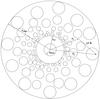Fig. 1 A schematic view of the wind model. rmin is the lower boundary of the wind (the surface of the star), rcl is the onset radius of the wind clumping, and rmax is the outer boundary of the calculation. Vectors r1, r2, and k are described in Sect. 3.2.

General method.

To solve the radiative transfer through the clumped wind, we first generate a snapshot of the clump distribution. Using the MC approach (see Sect. 3), we then follow the photons along their paths. The density and velocity of the wind can be arbitrarily defined in a 3D space. The calculations are carried out in the comoving frame following the prescriptions of Hamann (1980).

We solve the radiative transfer in the dimensionless form. We introduce the dimensionless frequency in the observer’s frame x^obs, which is measured relative to the line center in units of standard Doppler-width Δν_s${\mathit{x}}^{\mathrm{obs}}\mathrm{=}\left(\frac{\mathit{\nu }}{{\mathit{\nu }}_{\mathrm{0}}}\mathrm{-}\mathrm{1}\right)\frac{\mathit{c}}{{\nu }_{\mathrm{s}}}\mathit{,}$(1)where ν_s is an arbitrary reference velocity and ν_s = Δν_s(c/ν₀). During the calculations, we keep strictly the local co-moving frame frequency x^cmf of the photon, which means that the frequency of the followed photon at a certain coordinate point can be expressed using the scalar product of the vector of the local macroscopic velocity (ν) and the unit vector in the direction of the photon’s propagation (k) ${\mathit{x}}^{\mathrm{cmf}}\mathrm{=}{\mathit{x}}^{\mathrm{obs}}\mathrm{-}{k}\mathrm{·}\nu \mathit{.}$(2)Only when the photon exits the wind, x^cmf must be transformed into the observer’s frame by ${\mathit{x}}^{\mathrm{obs}}\mathrm{=}{\mathit{x}}^{\mathrm{cmf}}\mathrm{+}{k}\mathrm{·}\nu \mathit{.}$(3)Note that all velocities are dimensionless and measured in units of ν_s.

The code that we developed is gridless and does not require any symmetry. Instead of using a predefined grid, we introduce an adaptive integration step Δr. After choosing Δr, the velocity and opacity are calculated along the photon path. This allows us to account for arbitrary density and velocity inhomogeneities (for a detailed description see Sect. 3.2). For the vectors, we use Cartesian coordinates.

Basic assumptions.

To study the basic effects of clumping on the resonance line formation (both singlets and doublets), we adopt a core-halo model. Only the line opacity is taken into account, while the continuum opacity is neglected in the wind. We consider only pure scattering and assume complete redistribution. Only Doppler broadening is considered.

Wind velocity.

The velocity field can be arbitrary. For simplicity, we assume that the velocity field is radial and for the smooth wind we adopt the standard β-velocity law ${\nu }_{\mathit{r}}\mathrm{=}{\nu }_{\mathrm{\infty }}{\left(\mathrm{1}\mathrm{-}\frac{\mathit{b}}{\mathit{r}}\right)}^{\mathit{\beta }}\mathit{,}$(4)where ν_r is the radial component of the velocity vector, ν_∞ is the wind terminal velocity, and b is chosen such that ν_min ≤ 10^-3ν_∞.

The derivative of the Eq. (4) gives the radial velocity gradient ${\nu }^{\mathrm{\prime }}\mathrm{=}\frac{\mathrm{d}{\nu }_{\mathit{r}}}{\mathrm{d}\mathit{r}}\mathrm{=}{\nu }_{\mathit{r}}\hspace{0.17em}\mathit{\beta }\hspace{0.17em}\frac{\mathit{b}}{\mathit{r}\mathrm{(}\mathit{r}\mathrm{-}\mathit{b}\mathrm{)}}\mathit{,}$(5)which is important for choosing an adequate integration step.

Wind opacity.

A line opacity calculation in the moving medium requires that we take into account the Doppler shift, which leads to opacities that are anisotropic in the observer’s frame. We do not adopt the Sobolev approximation but solve the radiative transfer equation in the comoving frame. Since in this frame the fluid is at rest, the opacity is isotropic.

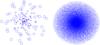Fig. 2 Two-dimensional projection of an example of a realisation of our stochastic 3D wind model. Left: clumps (blue circles) with the different size distributed around the star (red filled circle). Right: distribution of the clumps; the filled red sphere at the center represents the star, while the blue dots represent the positions of the clump centers.

For the opacity, we use the same parameterization as Hamann (1980)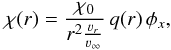$\mathit{\chi }\mathrm{\left(}\mathit{r}\mathrm{\right)}\mathrm{=}\frac{{\mathit{\chi }}_{\mathrm{0}}}{{\mathit{r}}^{\mathrm{2}}\frac{{\nu }_{\mathit{r}}}{{\nu }_{\mathrm{\infty }}}}\hspace{0.17em}\mathit{q}\mathrm{\left(}\mathit{r}\mathrm{\right)}\hspace{0.17em}{\mathit{\phi }}_{\mathit{x}}\mathit{,}$(6)where χ₀ is a free parameter of the model that corresponds to the line strength and is proportional to the mass-loss rate and abundance of the absorbing ion, q(r) reflects the depth-dependent degree of the ionization of the absorbing ion and for simplicity is chosen to be q(r) ≡ 1 here, i.e. constant ionization condition. The absorption profile φ_x for the singlet lines is assumed to be Gaussian ${\mathit{\phi }}_{\mathit{x}}\mathrm{=}\frac{\mathrm{1}}{\sqrt{\mathit{\pi }}}\hspace{0.17em}{\mathrm{e}}^{\mathrm{-}{\mathit{x}}^{\mathrm{2}}}\mathit{,}$(7)where x is the dimensionless frequency given by Eq. (1). We imply that the reference velocity ν_s is the Doppler-broadening velocity ν_D (i.e. ν_s = ν_D) that includes a contribution from both thermal broadening and microturbulence and is constant over the whole wind.

In this parametric formalism, the smooth wind opacity χ(r) is proportional to the smooth wind density ρ_sw(r). In our calculations, we do not directly calculate the wind density, but the depth-dependent line opacity χ(r), which is enough for calculation of the emergent radiation from the wind.

2.1. Description of clumping

2.1.1. Clump properties

Clumps are gaseous regions in the wind with higher density than their surroundings, and, possibly, also with different velocities from the smooth wind.

We allow for arbitrary optical depth of clumps. The clumps can be optically thick in the cores of a resonance lines, while they may remain optically thin at all other frequencies. Clumps are assumed to be stochastically distributed within the stellar wind. The average clump separation L(r) measured between their centers, is variable with the distance r from the star. For simplicity, we assume that each clump has the spherical shape with the volume (4π/3)l³, where l is the radius of the particular clump. The clump radius varies with the distance from the star, l = l(r). The density ρ_cl inside the clump at a distance r from the center is assumed to be higher by a factor D than the smooth wind density ρ_sw at the same radius ${\mathit{\rho }}_{\mathrm{cl}}\mathrm{\left(}\mathit{r}\mathrm{\right)}\mathrm{=}\mathit{D}\hspace{0.17em}{\mathit{\rho }}_{\mathrm{sw}}\mathrm{\left(}\mathit{r}\mathrm{\right)}$(8)and D ≥ 1. The factor D (density contrast) is the first free parameter of our model and for simplicity it is assumed to be depth independent. Using L and l, the factor D can be expressed as $\mathit{D}\mathrm{=}\frac{{\mathit{L}}^{\mathrm{3}}\mathrm{\left(}\mathit{r}\mathrm{\right)}}{\frac{\mathrm{4}\hspace{0.17em}\mathit{\pi }}{\mathrm{3}}{\mathit{l}}^{\mathrm{3}}\mathrm{\left(}\mathit{r}\mathrm{\right)}}\mathrm{·}$(9)In our model, clumps are assumed to be preserved entities. We assume that clumps are accelerated radially and neither split nor merge. The consequence of this is that the number of clumps per unit volume n_cl has to satisfy the equation of the continuity ${\mathit{n}}_{\mathrm{cl}}\mathrm{\propto }\frac{\mathrm{1}}{{\mathit{r}}^{\mathrm{2}}{\nu }_{\mathit{r}}}\mathrm{·}$(10)For the average clump separation, holds $\mathit{L}\mathrm{=}{\mathit{n}}_{\mathrm{cl}}^{\mathrm{-}\mathrm{1}\mathit{/}\mathrm{3}}$. With Eq. (10), this can be expressed as $\mathit{L}\mathrm{\left(}\mathit{r}\mathrm{\right)}\mathrm{=}{\mathit{L}}_{\mathrm{0}}\mathrm{3}\sqrt{{\mathit{r}}^{\mathrm{2}}\hspace{0.17em}4\mathrm{\left(}\mathit{r}\mathrm{\right)}}\mathit{,}$(11)where L₀ is a second free parameter of our model that represents the typical clump separation in units of the stellar radius, and 4(r) = ν_r/ν_∞ is the velocity in units of the terminal speed. As in the Eq. (11), the clump radius can be written as $\mathit{l}\mathrm{\left(}\mathit{r}\mathrm{\right)}\mathrm{=}{\mathit{l}}_{\mathrm{0}}\mathrm{3}\sqrt{{\mathit{r}}^{\mathrm{2}}\hspace{0.17em}4\mathrm{\left(}\mathit{r}\mathrm{\right)}}\mathit{,}$(12)where ${\mathit{l}}_{\mathrm{0}}\mathrm{=}{\mathit{L}}_{\mathrm{0}}\mathrm{3}\sqrt{\frac{\mathrm{3}}{\mathrm{4}\mathit{\pi D}}}\mathit{,}$(13)which follows from Eqs. (9) and (11). With this procedure, we create clumps whose size varies with the radial distance (see Fig. 2).

The volume filling factor f_V is defined as the ratio of the total volume that clumps occupy (V_cl) to the whole volume V_w in which the clumps are distributed (between r_cl and r_max), ${\mathit{f}}_{\mathit{V}}\mathrm{=}\frac{{\mathit{V}}_{\mathrm{cl}}}{{\mathit{V}}_{\mathrm{w}}}\mathrm{=}\frac{\sum _{\mathit{i}\mathrm{=}\mathrm{1}}^{{\mathit{N}}_{\mathrm{cl}}}{{\mathit{V}}_{\mathrm{cl}}}_{\mathit{i}}}{\frac{\mathrm{4}\mathit{\pi }}{\mathrm{3}}\mathrm{(}{\mathit{r}}_{\max }^{\mathrm{3}}\mathrm{-}{\mathit{r}}_{\mathrm{cl}}^{\mathrm{3}}\mathrm{)}}\mathit{,}$(14)where ${{\mathit{V}}_{\mathrm{cl}}}_{\mathit{i}}\mathrm{=}\mathrm{(}\mathrm{4}\mathit{\pi }\mathit{/}\mathrm{3}\mathrm{)}{\mathit{l}}_{\mathit{i}}^{\mathrm{3}}$ is the volume of ith clump and N_cl is the total number of the clumps.

For the case of void ICM, the entire mass of the wind in the clumps can be written as (using Eq. (8)) 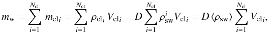${\mathit{m}}_{\mathrm{w}}\mathrm{=}\sum _{\mathit{i}\mathrm{=}\mathrm{1}}^{{\mathit{N}}_{\mathrm{cl}}}\hspace{0.17em}{{\mathit{m}}_{\mathrm{cl}}}_{\mathit{i}}\mathrm{=}\sum _{\mathit{i}\mathrm{=}\mathrm{1}}^{{\mathit{N}}_{\mathrm{cl}}}\hspace{0.17em}{{\mathit{\rho }}_{\mathrm{cl}}}_{\mathit{i}}\hspace{0.17em}{{\mathit{V}}_{\mathrm{cl}}}_{\mathit{i}}\mathrm{=}\mathit{D}\sum _{\mathit{i}\mathrm{=}\mathrm{1}}^{{\mathit{N}}_{\mathrm{cl}}}{\mathit{\rho }}_{\mathrm{sw}}^{\mathit{i}}{{\mathit{V}}_{\mathrm{cl}}}_{\mathit{i}}\mathrm{=}\mathit{D}\hspace{0.17em}\mathrm{⟨}{\mathit{\rho }}_{\mathrm{sw}}\mathrm{⟩}\sum _{\mathit{i}\mathrm{=}\mathrm{1}}^{{\mathit{N}}_{\mathrm{cl}}}{{\mathit{V}}_{\mathrm{cl}}}_{\mathit{i}}\mathit{,}$(15)where m_cli and ρ_cli are the mass and density of the ith clump, respectively, and ${\mathit{\rho }}_{\mathrm{sw}}^{\mathit{i}}$ is the value of the smooth wind density at the location of the ith clump. If the ICM is void, ${\mathit{f}}_{\mathit{V}}\mathrm{=}\frac{\mathrm{1}}{\mathit{D}}\mathrm{·}$(16)

2.1.2. Inter-clump medium

The ICM density ρ_ic is assumed to be lower than the smooth wind density ρ_sw (the density of the wind without any clumping) by a factor of d (the third free parameter of our model, which is assumed to be radius independent), and given by ${\mathit{\rho }}_{\mathrm{ic}}\mathrm{\left(}\mathit{r}\mathrm{\right)}\mathrm{=}\mathit{d}\hspace{0.17em}{\mathit{\rho }}_{\mathrm{sw}}\mathrm{\left(}\mathit{r}\mathrm{\right)}\mathrm{;} \mathrm{0}\mathrm{\le }\mathit{d}\mathit{<}\mathrm{1.}$(17)For a non-void ICM, the total mass of the wind is distributed between clumps and ICM. In this case, the total mass of the wind m_w =  ⟨ ρ_sw ⟩    V_w can be expressed as 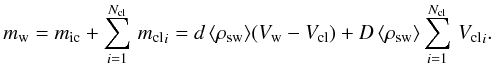${\mathit{m}}_{\mathrm{w}}\mathrm{=}{\mathit{m}}_{\mathrm{ic}}\mathrm{+}\sum _{\mathit{i}\mathrm{=}\mathrm{1}}^{{\mathit{N}}_{\mathrm{cl}}}\hspace{0.17em}{{\mathit{m}}_{\mathrm{cl}}}_{\mathit{i}}\mathrm{=}\mathit{d}\hspace{0.17em}\mathrm{⟨}{\mathit{\rho }}_{\mathrm{sw}}\mathrm{⟩}\mathrm{(}{\mathit{V}}_{\mathrm{w}}\mathrm{-}{\mathit{V}}_{\mathrm{cl}}\mathrm{)}\mathrm{+}\mathit{D}\hspace{0.17em}\mathrm{⟨}{\mathit{\rho }}_{\mathrm{sw}}\mathrm{⟩}\sum _{\mathit{i}\mathrm{=}\mathrm{1}}^{{\mathit{N}}_{\mathrm{cl}}}\hspace{0.17em}{{\mathit{V}}_{\mathrm{cl}}}_{\mathit{i}}\mathit{.}$(18)From Eqs. (14) and (18), it then follows that 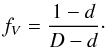${\mathit{f}}_{\mathit{V}}\mathrm{=}\frac{\mathrm{1}\mathrm{-}\mathit{d}}{\mathit{D}\mathrm{-}\mathit{d}}\mathrm{·}$(19)

2.1.3. Clump distribution

The distance r_i of the ith clump from the stellar center is chosen randomly by employing the von Neumann rejection method (Press et al. 1992) and assuming the inverse of the velocity law 1/ν_r to be as the probability density distribution function. This reflects the equation of the continuity for the number density of clumps. Consequently, more clumps are concentrated close to the star (see Fig. 2).

Clumps are distributed uniformly in cosθ_i and ϕ_i, and θ_i and ϕ_i are randomly chosen with $\cos {\mathit{\theta }}_{\mathit{i}}\mathrm{=}{\mathit{\mu }}_{\mathit{i}}\mathrm{=}\sqrt{{\mathit{\xi }}_{\mathit{i}\mathrm{1}}}$ and ϕ_i = 2πξ_i2 (where ξ_i1 and ξ_i2 are two different random numbers). For given r_i, the radius of each clump l_i is determined according to Eq. (12). We do not allow the clumps to overlap.

2.1.4. Inhomogeneous velocity in clumps

In our wind model the velocity of the smooth and the inter-clump medium is assumed to be monotonic as indicated in Eq. (4). However, the velocity inside the clumps is allowed to deviate from the monotonic wind and a negative velocity gradient can consequently appear (see more in the Sect. 3). This assumption is based on the prediction of hydrodynamic wind simulations (e.g. Owocki et al. 1988; Feldmeier et al. 1997b; Runacres & Owocki 2002), which show that over-dense regions inside the wind are slower and that ICM has approximately the same velocity as the smooth wind.

The velocity inside the ith clump can be approximated as 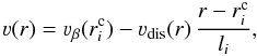$\nu \mathrm{\left(}\mathit{r}\mathrm{\right)}\mathrm{=}{\nu }_{\mathit{\beta }}\mathrm{\left(}{\mathit{r}}_{\mathit{i}}^{\mathrm{c}}\mathrm{\right)}\mathrm{-}{\nu }_{\mathrm{dis}}\mathrm{\left(}\mathit{r}\mathrm{\right)}\hspace{0.17em}\frac{\mathit{r}\mathrm{-}{\mathit{r}}_{\mathit{i}}^{\mathrm{c}}}{{\mathit{l}}_{\mathit{i}}}\mathit{,}$(20)where ${\mathit{r}}_{\mathit{i}}^{\mathrm{c}}$ is the absolute position of the center of the ith clump and ${\nu }_{\mathit{\beta }}\mathrm{\left(}{\mathit{r}}_{\mathit{i}}^{\mathrm{c}}\mathrm{\right)}$ is the velocity determined according to Eq. (4) at the position ${\mathit{r}}_{\mathit{i}}^{\mathrm{c}}$. The velocity dispersion ν_dis(r) = m   ν_β(r), where m (0 < m ≤ 1) is the velocity deviation parameter (fourth free parameter of our model). Equation (20) introduces a negative velocity gradient inside clumps, while the center of clump has the same velocity as the smooth wind. The velocity structure of our model along one particular photon path is shown in Fig. 3.

Fig. 3 Velocity structure of the wind model along the considered photon path for the case of a non-monotonic velocity distribution inside clumps.

3. Monte Carlo radiative transfer

The MC approach is the most promising way to treat radiation transfer in a clumped stellar wind. “Classical” solution methods for the radiative transfer equation, such as the Feautrier scheme or short characteristic methods, become extremely time and memory consuming and need very sophisticated solution schemes when we go to more spatial dimensions than one (e.g., Korčáková & Kubát 2003, 2005; Lobel & Blomme 2008). This is not the case for MC methods, where the extension to 2D or 3D is relatively simple.

3.1. Creation of a photon

A photon is released from the lower boundary of the wind (surface of the star) and then follows through the wind until it reaches the outer boundary of the wind or is scattered back into the photosphere. The photons are uniformly distributed in cosθ and ϕ over the whole surface area of the star. The photons from the lower boundary are released only upwards uniformly in ϕ and with a distribution function  ∝ μdμ in μ. The angular distribution function for photons emitted by the photosphere follows from the definition of the flux (see, e.g., Lucy 1983). The initial unit vector k of the photon propagation from the surface of the star is randomly chosen to have $\cos {\mathit{\theta }}_{\mathit{k}}\mathrm{=}{\mathit{\mu }}_{\mathit{k}}\mathrm{=}\sqrt{{\mathit{\xi }}_{\mathit{k}\mathrm{1}}}$ and ϕ_k = 2πξ_k2 (ξ_k1 and ξ_k2 are two different random numbers).

In our MC calculations, frequencies of newly created photons are determined from the interval defined using the ratio ν_∞/ν_D (as in Hamann 1981). The initial frequencies of photons have values in the interval  ⟨ x_min,x_max ⟩  where ${\mathit{x}}_{\min }\mathrm{=}\mathrm{-}\hspace{0.17em}\frac{{\nu }_{\mathrm{\infty }}}{{\nu }_{\mathrm{D}}}\hspace{0.17em}\mathrm{-}\hspace{0.17em}{\mathit{x}}_{\mathrm{band}}\mathit{,} {\mathit{x}}_{\max }\mathrm{=}\frac{{\nu }_{\mathrm{\infty }}}{{\nu }_{\mathrm{D}}}\hspace{0.17em}\mathrm{+}\hspace{0.17em}{\mathit{x}}_{\mathrm{band}}\mathit{,}$(21)and x_band is the line width, which is usually assumed to be about 4.5 Doppler units (as in Mihalas et al. 1975).

We divide the whole frequency interval into N_bin subintervals of equal length, and the same number of the photons are released in each subinterval. Each photon has the frequency ${\mathit{x}}_{\mathit{n}}^{\mathrm{obs}}\mathrm{\left(}{\mathit{r}}_{\min }\mathrm{\right)}$, which is randomly chosen from the frequency interval of nth (n = 1,...,N_bin) bin, given in the observer’s frame as ${\mathit{x}}_{\mathit{n}}^{\mathrm{obs}}\mathrm{\left(}{\mathit{r}}_{\min }\mathrm{\right)}\mathrm{=}\mathrm{(}\mathit{n}\mathrm{-}\mathit{\xi }\mathrm{)}{\mathit{x}}_{\mathrm{bin}}\mathrm{+}{\mathit{x}}_{\min }\mathit{,}$(22)where ${\mathit{x}}_{\mathrm{bin}}\mathrm{=}{}^{\mathrm{(}}\mathit{x}_{\max }\mathrm{-}{\mathit{x}}_{\min }{}^{\mathrm{)}}\mathit{/}{\mathit{N}}_{\mathrm{bin}}$ is the width of the frequency bin (the same for all bins) and ξ is a random number. The frequency is then transformed to the comoving-frame frequency ${\mathit{x}}_{\mathit{n}}^{\mathrm{cmf}}$.

3.2. Optical depth calculation

After its creation, each photon obtains information about how far it is allowed to travel before it undergoes interaction with some particle. This distance is determined by a randomly chosen optical depth τ_ξ =  −lnξ (see Avery & House 1968; Caroff et al. 1972). The actual optical depth that the photon passes on its travels, is calculated by summing the opacity contribution along its path, and compared to τ_ξ.

In order not to miss any inhomogeneities within the wind in either velocity or density, we use adaptive integration steps. The photon path is defined by the unit vector of photon propagation k and the photon is followed along its path by stepwise adding a variable integration step Δr. If the current photon position is r₁, then the vector of the next photon position r₂ is r₂ = r₁    +    Δr   k. After each integration step, the coordinates of the current photon position are recalculated. When the photon is followed through the smooth part of the wind, Δr is set to be no smaller than 0.1 of the radial length of the smooth wind region and no larger than ν_r/ν′, i.e., 0.1(r_cl − r_min) ≤ Δr ≤ ν_r/ν′, where ν′ is the velocity derivative (see Eq. (5)). When the photon is followed within the ICM, then Δr = 0.3   l(r₂), where l(r₂) is the radius that the clump would have at r₂ (Eq. (12)). For the photon path followed inside the clump, Δr is no smaller than 0.1   l(r₂) and no larger than 0.3   /ν′, i.e., 0.1l(r₂) ≤ Δr ≤ 0.3   /ν′. This adaptive integration step technique ensures that the opacity calculation along the photon path is done properly without any possibility of skipping an inhomogeneity within the wind and is fast enough. An illustration of the adaptive integration step is shown in Fig. 4.

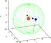Fig. 4 The path of one particular photon inside a realization of our clumped wind with the adaptive integration step. The bigger green sphere represents the outer boundary, while the red sphere in the center represents the lower boundary of the wind. Smaller blue balls represent the clumps and black dots denote integration steps.

For the optical depth calculation, it is necessary to know the opacity. According to Eq. (6), for the opacity calculation at the current position we need to know ν_r and the Doppler-shifted frequency of the photon at every position of the integration process. When the photon is traced within either the smooth or inter-clump regions, the velocity is calculated according to Eq. (4). When the photon is traced within the ith clump and the option of the inhomogeneous velocity is turned on (Sect. 2.1.4), then the velocity is calculated according to Eq. (20).

Along the photon path, the Doppler-shifted comoving-frame frequency of the photon is calculated.

The optical depth between r₁ and r₂ for the actual integration step j is ${\mathit{\tau }}_{\mathit{j}}\mathrm{=}{\mathrm{\int }}_{{\mathit{r}}_{\mathrm{1}}}^{{\mathit{r}}_{\mathrm{2}}}\mathit{\chi }\mathrm{\left(}\mathit{r}\mathrm{\right)}\mathrm{d}\mathit{r}$(23)and is calculated using the trapezoidal rule. Along the whole path, the optical depth is accumulated ($\mathit{\tau }\mathrm{=}{\sum }_{\mathit{j}}^{\mathit{J}}{\mathit{\tau }}_{\mathit{j}}$, where J is the total number of the integration steps made before scattering occurs), and when the total optical depth τ ≥ τ_ξ, then the condition for the line scattering is fulfilled.

After scattering, the photon obtains a new direction (θ,φ), chosen randomly for the case of isotropic scattering as cosθ = 2ξ − 1 and φ = 2πξ and a new optical depth τ_ξ =  −lnξ is randomly chosen again. For the determination of θ, φ, and τ_ξ, three different random numbers are used. Assuming a complete redistribution, the photon frequency after scattering is calculated randomly from a Gaussian distribution with the mean zero and the standard deviation unity (Box & Muller 1958).

To reproduce the emergent flux from the wind, all photons that reach the edge of the wind are collected and put into a proper frequency bin. Each of the profiles shown in this paper were calculated for one random configuration of clumps, which corresponds to an observation with a short exposure time relative to the dynamical timescale. On the other hand, we count the emergent photons irrespective of their direction, while the distant observer sees the 3D clump configuration from one specific direction. By averaging over all directions, we effectively obtain a mean emergent profile, similar to what we would get by averaging over many different random clump configurations but seen from one specific direction.

4. Results of the 3D wind model calculation

We demonstrate the basic effects on the line profiles of both single resonance lines and resonance doublets by varying different model parameters. Depending on the effect that we wish to study, some parameters are kept fixed, while others are varied within considered ranges (see Table 1). The basic model parameters (left part of Table 1) are chosen to represent a typical O type star. The varied model parameters (the right part of Table 1) have their default values except for the selected one whose effect we aim to study. The effects on the line profiles are shown for weak (χ₀ = 1), intermediate (χ₀ = 10), and strong (χ₀ = 100) lines. If the variation in some model parameter has a similar effect on all three types of lines, we show the effect for only the strong line case.

All calculations are performed using 10⁵ photons distributed over 100 frequency bins, resulting in a signal-to-noise ratio of about 30 per bin owing to the Poisson statistics.

4.1. The effects of the macroclumping

The total number of clumps in one snapshot of clump distribution can be derived using the parameter L₀ from ${\mathit{N}}_{\mathrm{cl}}\mathrm{=}\underset{{\mathit{r}}_{\mathrm{cl}}}{\overset{{\mathit{r}}_{\max }}{\mathrm{\int }}}{\mathit{n}}_{\mathrm{cl}}\mathrm{\left(}\mathit{r}\mathrm{\right)}\hspace{0.17em}\mathrm{4}\mathit{\pi }\hspace{0.17em}{\mathit{r}}^{\mathrm{2}}\hspace{0.17em}\mathrm{d}\mathit{r}\mathit{.}$(24)For instance, if 0.2 ≤ L₀ ≤ 0.5, then the total number of clumps within the clumped region is 10⁵ ≳ N_cl ≳ 10³. A larger number of clumps (i.e. smaller values of L₀) produces a less porous wind. If L₀ → 0, the whole wind is filled with many little clumps and resembles a smooth wind.

In this subsection, all model parameters are set to their default values except for χ₀ and L₀, which are varied as given in Table 1. The main macroclumping effect on the line profile is the reduction in the line strength relative to the smooth wind. In this case, where we assumed that clumping starts from the surface of the star (r_cl = 0), the variation in the L₀ parameter has a strong influence on all three types of lines (see the left part of Fig. 5). This is because the clumps are optically thick for these lines. However, if we assume that clumping starts at r_cl = 1.3, the clumps are optically thin for the weak lines there, while they are optically thick for the intermediate and strong line cases (see Šurlan et al. 2012).

According to Eqs. (12) and (13), the radius of the clumps depends on L₀. For very small L₀, a huge number of clumps with small radii are created, and the clump contribution to the line opacity is almost the same as in the case of a smooth wind. There are not too many “holes” between the clumps, and the photons cannot easily escape from the wind. However, for higher values of L₀, fewer clumps with larger radii exist. Consequently, there are more “holes” in the wind, through which photons may freely propagate. This leads to lower absorption and weaker lines.

Clumping lowers the effective opacity, to a lesser extent for the outer parts of the wind because the individual clumps become optically thin there, causing the bump in the blue part of the line. On the other hand, a significant part of the wind has approximately the same wind velocity close to the wind terminal velocity. Consequently, despite the lower effective opacity there is still enough matter to absorb. This causes the absorption dip near ν_∞, especially for lower L₀.

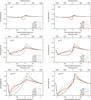Fig. 5 The effects of the macroclumping (left) and the non-void ICM (right) on the weak (χ0 = 1, the upper panels), intermediate (χ0 = 10, the middle panels), and strong (χ0 = 100, the lower panels) lines. Left: the black dashed lines represent a smooth wind (L0 → 0) and other lines are calculated for a different clump separation parameter L0 as given in the panels. Other model parameters have their default value (Table 1). Right: the black dashed lines represent a smooth wind and other lines are calculated for different values of the ICM density parameter d as given in the panels. Other model parameters have their default value (Table 1).

A similar effect of attenuation of the line strength can be obtained by varying the clumping factor D. In Fig. 6, we show the effect only for the strong line (χ₀ = 100). The model parameters are again set to their default values except that D is varied. When enhancing the density within clumps relative to the smooth wind density (i.e. increasing the parameter D), the porosity effect is more pronounced and the line becomes weaker.

4.2. Effects of the non-void inter clump medium

We now study the changes caused by variations in the ICM density parameter d and χ₀, when the other model parameters are set to their default values. The space between clumps is filled with matter of density defined by d. This matter fills the density “holes” between the clumps, and the photons can also be scattered there. This manifests itself as a strengthening of both the absorption and emission parts of the line profiles with respect to the model with void ICM (see the right part of Fig. 5). This effect is most pronounced for the strong lines, where even for a small d the ICM contributes a lot to the absorption coefficient and makes the lines more saturated and the emission parts stronger (see the right lower panel in Fig. 5). For the same value of the parameter d, the strong lines are saturated more than the intermediate lines. A proper choice of d can saturate the strong lines but still keep the intermediate lines unsaturated (e.g. see lines for d = 0.1 in the right middle and lower panels of Fig. 5).

Assuming that the ICM is not a void has an influence on the strength of the line as a whole, but has a particular effect on the center of the line, where a small absorption dip appears. Since more clumps are concentrated close to the star, the inner part of the wind together with the ICM contribute to the line opacity more than the outer part of the wind.

4.3. Effects of the onset of clumping

To illustrate the effect of varying the radius where clumping starts, we now fix all parameters of the model to their default values except for the onset radius of clumping r_cl. The main effect of the r_cl variation is the appearance of a strong absorption near the line center (see Fig. 7), which is due to the smooth part of the wind inside r_cl at low expansion velocity. If clumping starts higher in the wind, the absorption near the line center is broader and also partly attenuates the emission from the back hemisphere of the wind. This central absorption dip can therefore be used as a diagnostic for the onset of clumping.

We note that even a very small smooth part of the wind (between r = 1 and r = 1.01) causes significant central absorption, an effect that should be observable. As can be seen from Fig. 7, only when r_cl = 1 the absorption near the line center disappear. When the clumped part of the wind is larger (smaller value of the r_cl), the reduction in the line strength is more pronounced. By setting r_cl = r_max, the smooth wind is reproduced.

4.4. Effects of velocity dispersion inside clumps

The absorption of an individual clump can be broadened by stochastic (thermal or micro-turbulent) motions inside the clump, but also by an additional velocity gradient in the clump as predicted by hydrodynamic simulations. These kinds of line broadening are described in our model by the Doppler-broadening velocity (ν_D), and the velocity dispersion within the clumps (ν_dis), respectively (ses Sect. 2.1.4).

In Fig. 8, we show the effect of the ν_D variation. The normalization of the frequency-integrated absorption coefficient is maintained by a compensating change in χ₀. For a higher value of ν_D, the line profile is broader, and both the absorption and emission are stronger. When ν_D decreases, the macroclumping effect becomes more pronounced because the clumps are optically thicker in the line center, leading to a smaller effective optical depth due to a larger macroclumping effect.

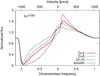Fig. 6 The effect of variation in the clumping factor D for the case of a strong line (χ0 = 100). The black dashed line represents a smooth wind, while the other lines are calculated for different D as given in the figure. Other model parameters have their default values (Table 1).

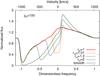Fig. 7 The effect of variation in the onset of the clumping rcl for the case of strong lines (χ0 = 100). The dashed black line represents the smooth wind (rcl = rmax) and other lines are calculated for different rcl as given in the figure. Other model parameters have their default value (Table 1).

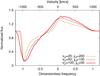Fig. 8 The effect of different Doppler broadening on the line profiles represented by three values of νD and χ0 as given in the figure. Other model parameters have their default value (Table 1).

To study the effect of the velocity dispersion within the clumps, we fix ν_D = 20   km   s^-1 and vary m and χ₀ (Fig. 9). If the velocity dispersion inside the clumps is higher (i.e. when increasing the parameter m), the gaps in the velocity field are smaller (more velocities overlap) and the probability of photon escape is lower. This leads to some absorption at velocities higher than ν_∞. However, in the example shown the velocity gradient inside the clumps does not differ much from the velocity gradient of the smooth wind except for its sign, thus leaving the optical depth of the individual clumps roughly the same. Therefore, the “vorosity” has only a small effect on the total line strength.

When the velocity dispersion is accounted for, the absorption extends to velocities higher than the terminal velocity ν_∞. This effect is important for the derivation of ν_∞ from observations (i.e. see Prinja et al. 1990), and may provide an effective diagnostic for the existence of the velocity dispersion inside the clumps.

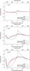Fig. 9 Effects of the velocity dispersion inside clumps on the line profile. Upper panel: weak lines (χ0 = 2.5), middle panel: intermediate lines (χ0 = 25), lower panel: strong lines (χ0 = 250). The black dashed lines represent the smooth wind, the green dashed lines (poro) represent pure porous wind, the other lines (poro+voro) represent the porous wind with non-monotonic velocity described with m as given in the panels. νD = 20   km   s-1 and other model parameters have their default values (Table 1).

4.5. Doublet calculation

For the calculation of doublets, the profile φ_x in Eq. (6) is assumed to have the form 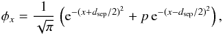${\mathit{\phi }}_{\mathit{x}}\mathrm{=}\frac{\mathrm{1}}{\sqrt{\mathit{\pi }}}\hspace{0.17em}\left({\mathrm{e}}^{\mathrm{-}\mathrm{(}\mathit{x}\mathrm{+}{\mathit{d}}_{\mathrm{sep}}\mathit{/}\mathrm{2}{\mathrm{)}}^{\mathrm{2}}}\mathrm{+}\mathit{p}\hspace{0.17em}{\mathrm{e}}^{\mathrm{-}\mathrm{(}\mathit{x}\mathrm{-}{\mathit{d}}_{\mathrm{sep}}\mathit{/}\mathrm{2}{\mathrm{)}}^{\mathrm{2}}}\right)\mathit{,}$(25)where d_sep is the separation between doublet components. The ratio of line opacities has a fixed value p = χ₁/χ₂, which follows from the atomic line strengths. The zero point frequency is located in-between the components.

The frequency of the photon after scattering is chosen randomly with a Gaussian distribution in the same way as for singlets. However, if the co-moving frame frequency of the photon before scattering indicates that it belongs to the blue component (x^cmf > 0), we assume that the photon is redistributed only within the blue component of the doublet, and vice versa.

In Fig. 10, we present one example of a strong doublet with d_sep = 2000   km   s^-1 and χ₀ = 500. We demonstrate the different effects on the line profile by changing the properties of the clumps. These effects are analogous to the single-line case. The main effect of macroclumping is a reduction in the line strength. If the velocity dispersion inside clumps is taken into account, there is some absorption at velocities higher than ν_∞. Only in the case of non-void ICM is it possible to saturate the line.

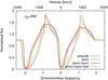Fig. 10 Effects of the macroclumping on the strong doublet line profiles (χ0 = 500) including non-void ICM and velocity dispersion inside clumps. The black dashed line represents the smooth wind, the green dashed line (poro) represents the macroclumping effect, the full red line (poro+voro) represents the macroclumping effect including non-monotonic velocity described inside clumps with m = 0.2, and the orange dash-dotted line (poro+voro+icm) represents the macroclumping effect including non-monotonic velocity with m = 0.2, and non-void ICM with d = 0.05. Other model parameters have their default values (Table 1).

5. Summary

We have presented a full 3D inhomogeneous stellar wind model and solved the radiative transfer to model the resonance lines. To our knowledge, this is the first work where the problem of resonance line formation in stellar winds is solved in full 3D, while previous work was restricted to 2D or pseudo-3D geometries only.

The radiative transfer is also calculated for the formation of doublets. This is important because UV resonance doublets are a key diagnostic for stellar winds. Our work demonstrates the role that stellar wind clumping plays in the formation of spectral lines, and how it affects the empirical wind diagnostics.

The method we develop here is very flexible, as is capable of accounting for the different 3D shapes of clumps, for arbitrary 3D velocity fields, and for the ICM at the same time. Below we briefly summarize the main results of our models, deferring the application to observed spectra to forthcoming work (Šurlan et al., in prep.).

• Allowing for clumps of any optical depths (macroclumping)causes a reduction in the effective opacity in the lines.Consequently, there is less absorption in the wind. Since thisreduction is weaker for the outer parts of the wind, the line profilesshow an absorption dip near ν_∞.

• For a given clumping factor D, the key model parameter affecting the effective opacity is L₀, the clump separation parameter. The opacity reduction is largest for the largest L₀ (Fig. 5). Therefore, the mass-loss rate empirically obtained by fitting the UV resonance lines becomes larger when the macroclumping effect is taken into account.

• The onset of clumping, r_cl, affects the line shape: the closer to the stellar surface clumping starts, the more pronounced is the absorption dip at the line center (Fig. 7). This absorption dip may provide an effective diagnostic for the onset of clumping.

• The line saturation is strongly affected by the ICM. A non-void ICM is required to reproduce the saturated lines simultaneously with non-saturated lines (Fig. 5).

• When accounting for a velocity dispersion within the clumps, when added to the mean velocity law, the absorption extends to a larger blue-shift than that corresponding to ν_∞. This effect has to be taken into account when deriving ν_∞ from observations.

• In any clumped wind, non-monotonic velocities will always appear together with the density inhomogeneities. Therefore, their combined effect must be taken into account for the line formation modeling.

• For resonance doublets, the clumping effects are analogous to those for single lines.

The main conclusion of our work is that in a realistic 3D wind with density inhomogeneities and non-stationary velocity, the P-Cygni profiles from resonance lines are different from those from smooth and stationary 3D winds. Any mass-loss diagnostics that do not account for wind clumping must underestimate the actual mass-loss rates. This can explain the reported discrepancies between the mass-loss rates obtained from ρ- and ρ²-based diagnostics, respectively. Using our general description of clumping presented in this work, it will be possible to determine improved values of the stellar mass-loss rates.

Acknowledgments

This work was supported by grants GA ČR 205/08/0003 and 205/08/H005, GA UK 424411, DAAD/AVČR D3-CZ2/2011-2012, and F.K.Z. 50 OR 1101 (LMO). The Astronomical Institute Ondřejov is supported by the project AV0 Z10030501. B.Š. thanks to Ministry of Education and Science of Republic of Serbia who supported this work through the project 176002 “Influence of collisions on astrophysical plasma spectra”. W.R.H. and L.M.O. are very grateful for the hospitality at the Ondřejov observatory. We thank the anonymous referee for useful suggestions regarding the clump distribution and other helpful remarks.

References

All Tables

All Figures

	Fig. 1 A schematic view of the wind model. rmin is the lower boundary of the wind (the surface of the star), rcl is the onset radius of the wind clumping, and rmax is the outer boundary of the calculation. Vectors r1, r2, and k are described in Sect. 3.2.
In the text

	Fig. 2 Two-dimensional projection of an example of a realisation of our stochastic 3D wind model. Left: clumps (blue circles) with the different size distributed around the star (red filled circle). Right: distribution of the clumps; the filled red sphere at the center represents the star, while the blue dots represent the positions of the clump centers.
In the text

	Fig. 3 Velocity structure of the wind model along the considered photon path for the case of a non-monotonic velocity distribution inside clumps.
In the text

	Fig. 4 The path of one particular photon inside a realization of our clumped wind with the adaptive integration step. The bigger green sphere represents the outer boundary, while the red sphere in the center represents the lower boundary of the wind. Smaller blue balls represent the clumps and black dots denote integration steps.
In the text

Fig. 5 The effects of the macroclumping (left) and the non-void ICM (right) on the weak (χ0 = 1, the upper panels), intermediate (χ0 = 10, the middle panels), and strong (χ0 = 100, the lower panels) lines. Left: the black dashed lines represent a smooth wind (L0 → 0) and other lines are calculated for a different clump separation parameter L0 as given in the panels. Other model parameters have their default value (Table 1). Right: the black dashed lines represent a smooth wind and other lines are calculated for different values of the ICM density parameter d as given in the panels. Other model parameters have their default value (Table 1).

In the text

	Fig. 6 The effect of variation in the clumping factor D for the case of a strong line (χ0 = 100). The black dashed line represents a smooth wind, while the other lines are calculated for different D as given in the figure. Other model parameters have their default values (Table 1).
In the text

	Fig. 7 The effect of variation in the onset of the clumping rcl for the case of strong lines (χ0 = 100). The dashed black line represents the smooth wind (rcl = rmax) and other lines are calculated for different rcl as given in the figure. Other model parameters have their default value (Table 1).
In the text

	Fig. 8 The effect of different Doppler broadening on the line profiles represented by three values of νD and χ0 as given in the figure. Other model parameters have their default value (Table 1).
In the text

Fig. 9 Effects of the velocity dispersion inside clumps on the line profile. Upper panel: weak lines (χ0 = 2.5), middle panel: intermediate lines (χ0 = 25), lower panel: strong lines (χ0 = 250). The black dashed lines represent the smooth wind, the green dashed lines (poro) represent pure porous wind, the other lines (poro+voro) represent the porous wind with non-monotonic velocity described with m as given in the panels. νD = 20   km   s-1 and other model parameters have their default values (Table 1).

In the text

Fig. 10 Effects of the macroclumping on the strong doublet line profiles (χ0 = 500) including non-void ICM and velocity dispersion inside clumps. The black dashed line represents the smooth wind, the green dashed line (poro) represents the macroclumping effect, the full red line (poro+voro) represents the macroclumping effect including non-monotonic velocity described inside clumps with m = 0.2, and the orange dash-dotted line (poro+voro+icm) represents the macroclumping effect including non-monotonic velocity with m = 0.2, and non-void ICM with d = 0.05. Other model parameters have their default values (Table 1).

In the text

References

- Avery, L. W., & House, L. L. 1968, ApJ, 152, 493 [NASA ADS] [CrossRef] [Google Scholar]
- Bouret, J.-C., Lanz, T., Hillier, D. J., et al. 2003, ApJ, 595, 1182 [NASA ADS] [CrossRef] [Google Scholar]
- Bouret, J.-C., Lanz, T., & Hillier, D. J. 2005, A&A, 438, 301 [NASA ADS] [CrossRef] [EDP Sciences] [Google Scholar]
- Bresolin, F., Crowther, P. A., & Puls, J. 2008, Massive Stars as Cosmic Engines, IAU Symp., 250 (Cambridge Univ. Press) [Google Scholar]
- Box, G. E. P., & Muller, M. E. 1958, Ann. Math. Statist., 29, 610 [Google Scholar]
- Caroff, L. J., Noerdlinger, P. D., & Scargle, J. D. 1972, ApJ, 176, 439 [NASA ADS] [CrossRef] [Google Scholar]
- Castor, J. I., Abbott, D. C., & Klein, R. I. 1975, ApJ, 195, 157 [NASA ADS] [CrossRef] [Google Scholar]
- Cranmer, S. R., & Owocki, S. P. 1996, ApJ, 462, 469 [NASA ADS] [CrossRef] [Google Scholar]
- Dessart, L., & Owocki, S. P. 2003, A&A, 406, L1 [NASA ADS] [CrossRef] [EDP Sciences] [Google Scholar]
- Dessart, L., & Owocki, S. P. 2005, A&A, 437, 657 [NASA ADS] [CrossRef] [EDP Sciences] [Google Scholar]
- Eversberg, T., Lépine, S., & Moffat, A. F. J. 1998, ApJ, 494, 799 [NASA ADS] [CrossRef] [Google Scholar]
- Feldmeier, A. 1995, A&A, 299, 523 [NASA ADS] [Google Scholar]
- Feldmeier, A., Kudritzki, R.-P., Palsa, R., Pauldrach, A. W. A., & Puls, J. 1997a, A&A, 320, 899 [NASA ADS] [Google Scholar]
- Feldmeier, A., Puls, J., & Pauldrach, A. W. A. 1997b, A&A, 322, 878 [NASA ADS] [Google Scholar]
- Feldmeier, A., Oskinova, L., & Hamann, W.-R. 2003, A&A, 403, 217 [NASA ADS] [CrossRef] [EDP Sciences] [Google Scholar]
- Fullerton, A. W., Massa, D. L., & Prinja, R. K. 2006, ApJ, 637, 1025 [NASA ADS] [CrossRef] [Google Scholar]
- Hamann, W.-R. 1980, A&A, 84, 342 [NASA ADS] [Google Scholar]
- Hamann, W.-R. 1981, A&A, 93, 353 [NASA ADS] [Google Scholar]
- Hamann, W.-R., & Koesterke, L. 1998, A&A, 335, 1003 [NASA ADS] [Google Scholar]
- Hamann, W.-R., & Gräfener, G. 2004, A&A, 427, 697 [NASA ADS] [CrossRef] [EDP Sciences] [Google Scholar]
- Hamann, W.-R., Brown, J. C., Feldmeier, A., & Oskinova, L. M. 2001, A&A, 378, 946 [NASA ADS] [CrossRef] [EDP Sciences] [Google Scholar]
- Hamann, W.-R., Oskinova, L. M., & Feldmeier, A. 2008, Clumping in Hot-Star Winds (Postdam, Germany: Universität Postdam) [Google Scholar]
- Hillier, D. J., & Miller, D. L. 1998, ApJ, 496, 407 [NASA ADS] [CrossRef] [Google Scholar]
- Korčáková, D., & Kubát, J. 2003, A&A, 401, 419 [NASA ADS] [CrossRef] [EDP Sciences] [Google Scholar]
- Korčáková, D., & Kubát, J. 2005, A&A, 440, 715 [NASA ADS] [CrossRef] [EDP Sciences] [Google Scholar]
- Krtička, J., & Kubát, J. 2007, ASP Conf. Ser., 361, 153 [NASA ADS] [Google Scholar]
- Krtička, J., & Kubát, J. 2009, MNRAS, 394, 2065 [NASA ADS] [CrossRef] [Google Scholar]
- Lépine, S., & Moffat, A. F. J. 1999, AJ, 514, 909 [Google Scholar]
- Lépine, S., & Moffat, A. F. J. 2008, AJ, 136, 548 [NASA ADS] [CrossRef] [Google Scholar]
- Lobel, A., & Blomme, R. 2008, ApJ, 678, 408 [NASA ADS] [CrossRef] [Google Scholar]
- Lucy, L. B. 1983, ApJ, 274, 372 [NASA ADS] [CrossRef] [Google Scholar]
- Lucy, L. B., & Solomon, P. M. 1970, ApJ, 159, 879 [NASA ADS] [CrossRef] [Google Scholar]
- Lucy, L. B., & White, R. L. 1980, ApJ, 241, 300 [NASA ADS] [CrossRef] [Google Scholar]
- Maeder, A., & Meynet, G. 2010, New Astron. Rev., 54, 32 [NASA ADS] [CrossRef] [Google Scholar]
- Markova, N., Puls, J., Scuderi, S., & Markov, H. 2005, A&A, 440, 1133 [NASA ADS] [CrossRef] [EDP Sciences] [Google Scholar]
- Massa, D., Prinja, R. K., & Fullerton, A. W. 2008, in Clumping in hot-star winds, ed. W.-R. Hamann, A. Feldmeier, & L. M. Oskinova (Postdam, Germany: University Postdam), 147 [Google Scholar]
- Mihalas, D., Heasley, J. N., & Auer, L. H. 1975, NCAR-TN/STR-104 [Google Scholar]
- Muijres, L., de Koter, A., Vink, J., et al. 2011, A&A, 526, A32 [Google Scholar]
- Mullan, D. J. 1984, ApJ, 283, 303 [NASA ADS] [CrossRef] [Google Scholar]
- Oskinova, L. M., Feldmeier, A., & Hamann, W.-R. 2004, A&A, 422, 675 [NASA ADS] [CrossRef] [EDP Sciences] [Google Scholar]
- Oskinova, L. M., Feldmeier, A., & Hamann, W.-R. 2006, MNRAS, 372, 313 [NASA ADS] [CrossRef] [Google Scholar]
- Oskinova, L. M., Hamann, W.-R., & Feldmeier, A. 2007, A&A, 476, 1331 [NASA ADS] [CrossRef] [EDP Sciences] [Google Scholar]
- Owocki, S. P. 2008, in Clumping in Hot Star Winds, 121 [Google Scholar]
- Owocki, S. P. 2010, ASP Conf. Ser., 425, 199 [NASA ADS] [Google Scholar]
- Owocki, S. P., Castor, J. I., & Rybicki, G. B. 1988, ApJ, 335, 914 [NASA ADS] [CrossRef] [Google Scholar]
- Owocki, S. P., & Cohen, D. H. 2006, ApJ, 648, 565O [NASA ADS] [CrossRef] [Google Scholar]
- Press, W. H., Teukolsky, S. A., Vetterling, W. T., & Flannery, B. P. 1992, Numerical Recipes in FORTRAN: The Art of Scientific Computing, 2nd edn. (New York: Cambridge University Press) [Google Scholar]
- Pauldrach, A., Puls, J., & Kudritzki, R.-P. 1986, A&A, 164, 86 [NASA ADS] [Google Scholar]
- Prinja, R. K., & Howarth, I. D. 1986, ApJS, 61, 357 [NASA ADS] [CrossRef] [Google Scholar]
- Prinja, R. K., & Massa, D. L. 2010, A&A, 521, L55 [Google Scholar]
- Prinja, R. K., Barlow, M. J., & Howarth, I. D. 1990, ApJ, 361, 607 [NASA ADS] [CrossRef] [Google Scholar]
- Puls, J., Urbaneja, M. A., Venero, R., et al. 2005, A&A, 435, 669 [NASA ADS] [CrossRef] [EDP Sciences] [Google Scholar]
- Puls, J., Vink, J. S., & Najarro, F. 2008, A&AR, 16, 209 [Google Scholar]
- Runacres, M. C., & Owocki, S. P. 2002, A&A, 381, 101 [Google Scholar]
- Sundqvist, J. O., Puls, J., & Feldmeier, A. 2010, A&A, 510, 11 [Google Scholar]
- Sundqvist, J. O., Puls, J., Feldmeier, A., & Owocki, S. P. 2011, A&A, 528, 64 [Google Scholar]
- Šurlan, B., Hamann, W.-R., Kubát, J., Oskinova, L. M., & Feldmeier, A. 2012, Four Decades of Research on Massive Stars, ed. C. Robert, N. St-Louis, & L. Drissen, ASP Conf. Ser., in press [Google Scholar]
- Waldron, W. L., & Cassinelli, J. P. 2010, ApJ, 711, L30 [NASA ADS] [CrossRef] [Google Scholar]
- Whitney, B. A. 2011, Bull. Astron. Inst. India, 39, 101 [Google Scholar]
- Zsargó, J., Hillier, D. J., & Bouret, J.-C., et al. 2008, A&A, 685, L149 [Google Scholar]
All Tables
The model parameters to study the influence of their variation on the resonance line profiles.