| Issue |
A&A
Volume 541, May 2012
|
|
|---|---|---|
| Article Number | A95 | |
| Number of page(s) | 12 | |
| Section | Interstellar and circumstellar matter | |
| DOI | https://doi.org/10.1051/0004-6361/201117677 | |
| Published online | 07 May 2012 | |
Probing the anomalous extinction of four young star clusters: the use of colour-excess, main-sequence fitting and fractal analysis⋆
1 Universidade de São Paulo, IAG, rua do Matão 1226, 05508-900 São Paulo, Brazil
e-mail: bfernandes@astro.iag.usp.br
2 Universidade Federal do ABC, CECS, rua Santa Adélia 166, 09210-170 Santo André, SP, Brazil
Received: 10 July 2011
Accepted: 22 February 2012
Aims. We studied four young star clusters to characterise their anomalous extinction or variable reddening and asses whether they could be due to contamination by either dense clouds or circumstellar effects.
Methods. We evaluated the extinction law (RV) by adopting two methods: (i) the use of theoretical expressions based on the colour-excess of stars with known spectral type; and (ii) the analysis of two-colour diagrams, where the slope of the observed colour distribution was compared to the normal distribution. An algorithm to reproduce the zero-age main-sequence (ZAMS) reddened colours was developed to derive the average visual extinction (AV) that provides the closest fit to the observational data. The structure of the clouds was evaluated by means of a statistical fractal analysis, designed to compare their geometric structure with the spatial distribution of the cluster members.
Results. The cluster NGC 6530 is the only object of our sample affected by anomalous extinction. On average, the other clusters suffer normal extinction, but several of their members, mainly in NGC 2264, seem to have high RV, probably because of circumstellar effects. The ZAMS fitting provides AV values that are in good agreement with those found in the literature. The fractal analysis shows that NGC 6530 has a centrally concentrated distribution of stars that differs from the substructures found in the density distribution of the cloud projected in the AV map, suggesting that the original cloud was changed by the cluster formation. However, the fractal dimension and statistical parameters of Berkeley 86, NGC 2244, and NGC 2264 indicate that there is a good cloud-cluster correlation, when compared to other works based on an artificial distribution of points.
Key words: dust, extinction / stars: pre-main sequence / methods: statistical
Appendix is available in electronic form at http://www.aanda.org
© ESO, 2012
1. Introduction
Extinction is one of the most well-known consequences of the dust present in the interstellar medium (ISM). The study of the effects of extinction on star-forming regions reveals properties of the interstellar material that helps to improve our understanding of the formation and evolution of stars.
Each line-of-sight has an extinction-law value that is characterised by the ratio of the total-to-selective extinction RV = AV/E(B − V) and depends on the composition of the ISM. According to Savage & Mathis (1979), the average value of this ratio in the diffuse ISM is 3.1, while in denser regions it might reach values in the range 4 < RV < 6. Anomalous extinction laws have been found in several star-forming regions (Neckel & Chini 1981; Chini & Krugel 1983; Chini & Wargau 1990; Pandey et al. 2000; Samal et al. 2007). In addition to the differences in the ISM characteristics, common explanations of high values of RV are the selective evaporation of small grains by the radiation from hot stars, and grain growth in circumstellar environments (e.g. van den Ancker et al. 1997). The circumstellar hypothesis seems to be supported by the correlation between reddening and extinction found by Sung et al. (2000) for a sample of 30 stars. Most of these objects had their SED well-fitted by assuming that RV = 3.1, with some exceptions that show anomalous RV and have high extinction probably owing to the circumstellar material. From the results of a polarimetric survey in the direction of the Lagoon Nebula (M8), McCall et al. (1990) estimated that RV = 4.64 ± 0.27, which they attributed to circumstellar effects. This anomalous RV was obtained after removing the normal foreground extinction.
The dependence of the extinction law on wavelength has also been widely discussed in the literature, given the interest in identifying the characteristics of different types of grains causing the extinction, as well as the need to properly correct the reddening affecting the observational data. In general, a power law is adopted as the “universal extinction law” for wavelengths longer than 1 μm. The power law (Aλ ∝ λ − β) fits most extinction curves. However, it is recognised that the index β depends significantly on the line-of-sight. Fitzpatrick & Massa (2009) used data from the Hubble Space Telescope to investigate the extinction dependence on near-infrared (near-IR) wavelengths. They found that a “universal” law does not apply in this case and that the index β tends to decrease with increasing RV. Instead of extrapolating the usual power law, Fitzpatrick & Massa (2009) suggest a different form, one independent of wavelength, that more closely describes the near-IR extinction (see discussion in Sect. 3.1).
One of the most important issues directly affected by the correct determination of extinction is the accuracy of the distance estimation. The cluster NGC 3603, for instance, has distances found in the literature varying from 6.3 kpc to 10.1 kpc, a discrepancy mostly due to errors in the reddening correction. Adopting the normal RV, Melena et al. (2008) estimated a distance of 9.1 kpc for NGC 3603, while a distance of 7.6 kpc was found when they assumed the anomalous extinction law RV = 4.3 proposed by Pandey et al. (2000). The correct determination of distance is crucial to the estimation of physical parameters of open clusters, such as stellar masses and ages. In star-forming regions, special attention must be paid to the probable occurrence of either anomalous or differential extinction.
Several methods can be employed to estimate the interstellar extinction in the direction of young star clusters, which can be due to different effects: (i) the foreground in a given line-of-sight that is pervaded by interstellar material in-between the cluster and the observer; (ii) the presence of a dark cloud associated to the cluster; and (iii) the individual extinction caused by circumstellar material.
The use of a U − B versus (vs.) B − V colour–colour diagram is the classical method for estimating the average extinction towards open clusters (e.g. Prisinzano et al. 2011) and it is especially useful when there is a lack of spectroscopic observations (e.g. Jose et al. 2011).
In addition to colour–colour diagrams in the UBV bands, Chini & Wargau (1990) propose that two-colour diagrams (TCDs) are also interesting for the study of extinction. These diagrams are presented in the form V − λ × B − V, where λ refers to different bands. The distribution of the stars in TCDs is roughly linear. Anomalies in the extinction law are determined by comparing the distribution of field stars (which follows a normal extinction law) with the distribution of the cluster members (which may follow an anomalous extinction law).
Jose et al. (2008) adopted TCDs to verify the extinction law in the direction of the cluster Stock 8, for instance. They found the same slope for the inner region of the cluster (r < 6′) as for a larger area (r < 12′), which also includes field stars. Another example is the cluster NGC 3603 for which Pandey et al. (2000) estimated that RV = 4.3, indicating that there is a remarkable difference between the distributions of field stars and members of the cluster in the TCDs.
The aim of the present work is to characterise the extinction in the direction of different young star clusters, by determining the extinction law and searching for possible spatial variations. We selected four well-known clusters, whose characteristics are compiled in the Handbook of Star forming regions edited by Bo Reipurth (2008): Berkeley 86 is found in the Cygnus OB1 region (Reipurth & Schneider 2008); NGC 2244 is associated with the Rosette Nebula (Róman-Zúñiga & Lada 2008); NGC 2264 is related to the Mon OB1 association (Dahm 2008); and NGC 6530 is located near to the Lagoon Nebula (Tothill et al. 2008).
The motivation in choosing these well-known objects is to refine the previous extinction determinations, by adopting the same criteria for the selection and analysis of data sets, in order to compare our results with the characteristics of the cluster environments. The paper is organised as follows. Section 2 presents the sample and the information available in the literature for the members of the clusters and the clouds associated with them. Different methods are adopted in Sect. 3, which are designed to estimate RV in the direction of the clusters. Section 4 describes an automatic method to fit the ZAMS reddened colours to the observed data, providing an accurate estimation of visual extinction. In Sect. 5, we develop an analysis of the fractal dimension of the clouds by comparing the spatial distribution of cluster members with statistical parameters related to clustering. The discussion of the results and the conclusions are presented in Sect. 6. The colour diagrams utilised to study the extinction are presented in Appendix A.
List of the studied clusters.
2. Description of the sample
The list of clusters and their main characteristics are given in Table 1. This section is dedicated to summarising the information found in the literature, and to describing the adopted criteria used to select the cluster members and their available observational data. We also performed an analysis of visual extinction maps and far-IR images of clouds against which the clusters are projected.
2.1. Selected clusters
Berkeley 86 is a particularly small cluster associated with the Cygnus OB1 region. Its youth was revealed by the discovery of O type stars by Sanduleak (1974). Bhavya et al. (2007) found a distance of 1585 ± 160 pc. They suggest that a low-level star-formation episode occurred 5 Myr ago, and that another more vigorous one has started in the past 1 Myr. Reipurth & Schneider (2008) compare the gas and dust distributions in the Cygnus X region, which is influenced by the UV radiation from the OB1 association (see their Fig. 3). They show that Berkeley 86 is isolated and projected against an area totally free of gas and dust, which is indicative of low levels of extinction for this cluster. Yadav & Sagar (2001) found that Berkeley 86 suffers non-uniform reddening with colour-excess varying in the range 0.24 < E(B − V) < 1.01, while Forbes (1981) measured a more uniform estimation of E(B − V) = 0.96 ± 0.07.
NGC 2244 is located at the centre of the Rosette Nebula. It is a prominent OB association that is probably responsible for the evacuation of the central part of the nebula. The first photometric study of this cluster (Johnson 1962) measured a colour-excess E(B − V) = 0.46 assuming RV = 3.0, a result that was later confirmed by Turner (1976) and Ogura & Ishida (1981). Pérez et al. (1987) found an anomalous RV for some of the cluster members and suggested main-sequence (MS) and pre-MS stars coexist. Róman-Zúñiga & Lada (2008) suggested ages of 3 ± 1 Myr. Wang et al. (2008) studied the X-ray sources detected by Chandra in the Rosette region. They verified a double structure in the stellar radial density profile, suggesting that NGC 2244 is not in dynamical equilibrium.
NGC 2264 is one of the richest clusters in terms of mass range, and has a well-defined pre-MS (Dahm 2008). The estimated ages vary from 0.1 Myr to 10 Myr (Flaccomio et al. 1997; Rebull et al. 2002). Surveys in Hα and X-rays revealed about 1000 members. The cluster is observed projected against a molecular cloud complex of ~2° × 2° and is located 40′ north of the Cone Nebula. The interstellar reddening on this cluster is believed to be low: AV = 0.25 estimated by Walker (1954) adopting E(B − V) = 0.082 and RV = 3.08. Rebull et al. (2002) derived AV = 0.45 from a spectral study of a sample of more than 400 stars. Alencar et al. (2010) used the CoRoT satellite to perform a synoptical analysis of NGC 2264 with high photometric accuracy. Their results are indicative of a dynamical star-disc interaction among the cluster members, indicating that they are young accreting stars.
In the study by Tothill et al. (2008) of the Lagoon Nebula and its surroundings, particular emphasis is given to NGC 6530, which is a star cluster associated with an HII region that lies at about 1300 ± 100 pc. The estimated age of NGC 6530 is less than 3 Myr (Arias et al. 2007). Despite being along a line-of-sight that contains a high concentration of gas, NGC 6530 appears to be decoupled from the molecular cloud once the cluster members do not seem to be very embedded. This implies that NGC 6530 is inside the cavity of the HII region (McCall et al. 1990), as indicated by measurements of the expanding gas (Welsh 1983). A range of 0.17 mag to 0.33 mag has been reported for the colour-excess in the direction of NGC 6530 (Mayne & Naylor 2008). van den Ancker et al. (1997) found a normal extinction law for the intra-cluster region, while Arias et al. (2007) proposed that RV = 4.6 for some of the embedded stars. Anomalous extinction has also been reported for individual cluster members, for instance the star HD 164740, for which Fitzpatrick & Massa (2009) suggest that E(B − V) = 0.86 and 5.2 < RV < 6.1.
2.2. Data extraction and cluster membership
Two main catalogues of open clusters can be found in the literature: (i) the WEBDA1 database; and (ii) the catalogue DAML022 by Dias et al. (2002b) with the compilations Tables of membership and mean proper motions for open clusters of Dias et al. (2002a) based on TYCHO2 and Dias et al. (2006) based on the UCAC2 catalogue.
From DAML02, we searched for clusters with ages of up to 10 Myr and distances of up to 2 kpc, only selecting those that had members with UBVI photometry and spectral classification available in the WEBDA database. A summary of the characteristics of the sample selected from these two databases is listed in Table 1.
To search for relevant information about stars located in the direction of the clusters, three data sets were extracted from WEBDA: (i) UB photometry; (ii) VI photometry; and (iii) equatorial coordinates (J2000). Each source has the same identification in all of these data sets, but the photometry is derived from different studies. To ensure consistency in the data analysis, we selected only members with UBVI photometry provided by a single work. The number of studied stars and the corresponding references to the photometric catalogues are listed in Table 2, which also gives information on the number of stars with available spectral data.
According to Yadav & Sagar (2001), the correct identification of members is crucial for the assessment of extinction in the direction of the cluster and the most reliable selection is based on kinematic studies (proper motion and radial velocity). DAML02 provides a list of stars with JHK photometry – 2MASS catalogue (Cutri et al. 2003) – and also the probability of the star belonging to the cluster (P%), which is determined from its proper motion. To verify wether P% is available for our WEBDA sample, their coordinates were compared with those listed by DAML02. A coincidence of sources was only accepted for objects with less than 5 arcsec of difference between coordinates.
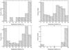 |
Fig. 1 Normalised number of stars distributed according to membership probability (P%), which is based on their proper motion. A dotted line indicates the minimum probability (Pmin) that was adopted to separate the most probable members from field stars. Top: Berkeley 86 (left) and NGC 2244 (right). Bottom: NGC 2264 (left) e NGC 6530 (right). |
The distribution of the number of stars as a function of P% was evaluated on the basis of the histograms presented in Fig. 1. A bimodal distribution is verified, enabling us to distinguish between members and possible field stars. As proposed by Yadav & Sagar (2001), the pollution by field stars should be smaller if only stars with high values of P% are considered members of the cluster. For each cluster, a minimum probability (Pmin) was adopted to help distinguish field stars, as indicated by the dotted lines in the histograms in Fig. 1.
The spatial distribution of the stars was also checked by looking for possible preferential concentrations, as a function of P%. However, no trend was found in the member distribution.
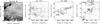 |
Fig. 2 Map of visual extinction over-imposed by contours measured from IRIS-IRAS images at 100 μm band. The contours vary from 50–350 MJy/Sr with steps of 100 MJy/Sr, except for NGC 6530 that has contours starting at 500 MJy/Sr with steps of 1000 MJy/Sr. The area of the cluster is indicated by the black central square. |
2.3. Comparison with molecular clouds
Extinction caused by interstellar dust detected along the line-of-sight can be determined by models that reproduce the stars counts in the Galaxy (e.g. Amôres & Lépine 2005) or maps of visual extinction (Gregorio-Hetem et al. 1988; Schlegel et al. 1998; Dobashi et al. 2005, among others). More recently, colour-excess maps obtained from near-IR surveys have been used to derive the visual extinction in the direction of molecular clouds, as for instance the Trifid nebula studied by Cambrésy et al. (2011) based on 2MASS, UKIDSS, and Spitzer data.
Figure 2 displays the position of each cluster projected against the visual extinction map obtained from the 2MASS data (K band). The catalogue of dark clouds by Dobashi et al. (2005) was used to extract the maps for the regions containing our clusters. To compare the extinction with the far-IR flux density of the clouds, the AV maps are over-imposed by contours of IRAS-IRIS data at 100 μm. A significant variation in both AV and far-IR emission can be found in the direction of the clusters, except for Berkeley 86 that appears projected against a uniform field. High levels of far-IR emission are found in the direction of the clusters NGC 6530 and NGC 2264, which coincide with dense regions in the AV maps. Table 1 gives the range of flux at 100 μm and AV in the direction of the clusters. In spite of the substructures of the clouds being more evident in K band, we adopted the optical (DSS) maps from Dobashi et al. (2005) to measure AV.
3. Study of the extinction law
3.1. RV estimation based on colour-excess
One method developed to obtain RV uses colour-excess, which can be determined for each cluster member that has a well-known spectral type. Intrinsic colours were adopted from Bessell et al. (1998), based on values of surface gravity and effective temperature that were respectively extracted from Straizys & Kuriliene (1981) and de Jager & Nieuwenhuijzen (1987) as a function of the spectral type and luminosity class available for some stars of the sample.
The expression  was adopted from Cardelli et al. (1989) in order to derive relations between RV and colour-excess. The results are similar to those based on van de Hulst’s theoretical extinction (e.g. Johnson 1968). According to Fitzpatrick & Massa (2009), these theoretical curves seem to be valid only for low-to moderate values of RV, which tend to be underestimated in the case of anomalous extinction laws. They suggested a new formula
 ![\hbox{$R_{\rm V}[K] = 1.36 \frac{E(V-K)}{E(B-V)} - 0.79$}](/articles/aa/full_html/2012/05/aa17677-11/aa17677-11-eq54.png) , which more closely reproduces the extinction law along different lines of sight.
, which more closely reproduces the extinction law along different lines of sight.
Owing to a lack of spectral type information for our entire sample, we did not determine RV for each cluster member. We compared instead the expected ranges of RV as a function of the distribution of colour-excesses with the theoretical extinction laws in the E(V − K) × E(B − V) plot presented in Fig. 3. An illustration of the dispersion found for RV[K] = 6 is shown by the hatched area, corresponding to the extinction laws given by Cardelli et al. (1989) (upper line) and Fitzpatrick & Massa (2009) (lower line). For RV[K] < 4, the theoretical lines from both works are quite similar.
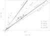 |
Fig. 3 Different extinction laws compared to the colour-excess distribution for cluster members with available spectral types. Error bars illustrate the maximum uncertainty expected, if the spectral type is not well-determined, for a G8 star. |
Considering the few objects with a known spectral type, this analysis cannot be conclusive for our sample, but gives some indication of the variation in both E(B − V) and RV for each cluster. NGC 2264 shows the largest variation, with E(B − V) ranging from 0.01 to 0.3 mag as measured for a sub-sample of 20 stars. A degenerate distribution of RV is found in this case, spreading from 2.1 to >6. It can be seen in Fig. 3 that NGC 2264 seems to have a bimodal distribution, where part of the members follows the normal extinction law, while another part has RV > 6.
There are several possible causes of the large variations found in NGC 2264: (i) observational problems that would give inaccurate optical photometry or spectral type determination; (ii) actual variations in each line-of-sight around the cluster area; and (iii) anomalies caused by the circumstellar environment. In principle, the two first options may be disregarded, since the observational information has been checked in other data sets. Furthermore, there is no correlation between the position of a given cluster member and its RV. We conclude that circumstellar matter seems to explain more clearly the anomalies. It can also be noted in Fig. 3 that E(V − K) is particularly large for seven objects in NGC 2264, which is inconsistent with the low E(B − V) values and suggests a K band excess usually found in the presence of circumstellar matter. Six of these stars have spectral types later than A0, for which it is important to take into account the errors in the spectroscopic data that may cause significant uncertainties in the colour excess (see Sect. 3.3). However, we note that some of these objects also show an offset from the normal distribution of the observed colours in TCDs (see Sect. 3.2 and Fig. A.2), which is more consistent with individual anomalies in RV than possible errors in photometry.
Smaller variations are found for the other clusters: members of NGC 2244 have RV[K] ~ 3.1, NGC 6530 shows a trend to slightly larger values (3.1 < RV[K] < 4), and Berkeley 86 tends to have lower values (2.7 < RV[K] < 3). However, these results are based on few stars and need to be confirmed by different methods of RV estimation.
3.2. Two-colour diagrams
To search for anomalies in the extinction law, we also constructed TCDs following the method proposed by Chini et al. (1983, 1990) and more recently used by Pandey et al. (2000), Jose et al. (2008), Chauhan et al. (2011), and Eswaraiah et al. (2012), among others. These TCDs can be used to perform a qualitative analysis of the nature of the extinction by using the relation Rc = Rn × (ac/an), where Rn is the normal extinction law, ac is the slope of the linear fit for the cluster members, and an is the slope for field stars.
Our TCDs use V − λ colours, where λ represents the IJHK bands. In these diagrams, the intrinsic colours follow a linear distribution up to B − V ~ 1. This limit defines a restricted spectral range of validity, where the ZAMS distribution corresponds to a straight line. In the TCDs, the distribution of field stars is well-reproduced by the ZAMS intrinsic colours, once they are reddened by using the mean E(B − V) estimated in the direction of the cluster. In this case, our ZAMS fitting was obtained with RV = 3.1, which we adopted to simulate the distribution of the field stars that must be compared to the cluster members.
The fitting of our sample is restricted to the cluster members for which P% > Pmin, which helps to avoid confusion with field stars. Since the TCD analysis is valid only for a very narrow range of B − V, our calculations are based on objects with spectral type earlier than B8. For each studied band, the slope of the linear fit for the selected cluster members (ac) was compared to the slope of the normal ZAMS distribution (an).
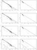
Figures A.1 and A.2 show the diagrams V − I,V − J,V − H, and V − K vs. B − V, for which an is 1.09 ± 0.02, 1.87 ± 0.03, 2.42 ± 0.03, and 2.51 ± 0.04, respectively. The effect of reddening combined with anomalous extinction is illustrated in the V − K vs. B − V diagrams, where extinction vectors were plotted to represent AV = 2 mag for two choices of RV similar to those used, for instance, by Da Rio et al. (2010).
Table 2 presents our results for the TCD analysis giving the fitted line slope in each band, which is used to estimate the mean RV obtained for the early-type stars. Within the estimated errors, good agreement is found in all bands, except for NGC 6530. In this case, RV ranges from 4.5 to 6.2. This is the only cluster of the sample clearly showing an anomalous extinction law with a significant dependence on wavelength. Berkeley 86 and NGC 2264 seems to follow a normal law. As verified in Sect. 3.1 (Fig. 3), NGC 2244 also has a bimodal distribution in the TCDs: some of the objects follow the normal law, while others have anomalous extinction.
Extinction laws from literature and results obtained from the TCD analysis.
3.3. Error estimation
Since our work is based on photometric and spectroscopic data from literature, we evaluated the global uncertainties taking into account the different sources of errors.
According to the references that provided the photometric data (see Table 2), the error in the magnitudes and colours is ~0.08 mag at worst. Since this value is smaller than the symbol size in the colour–colour diagrams (see Figs. A.1 and A.2), it did not affect the linear fitting used to estimate the variations in the extinction law.
Most objects with known spectral types in our sample are O or B type stars, whose errors in the characterisation of spectral types are insignificant in our calculation of colour-excess. The only exception is NGC 2264, which contains some A, F, or G stars for which we adopted a maximum uncertainty of two spectral subtypes.
By combining both spectroscopic and photometric errors, to derive colour-excess, we estimated the maximum deviation (at worst) of 0.3 mag in E(B − V) and 0.4 mag in E(V − K) for a G8 type star of NGC 2264. Since we do not use the colour-excess to derive the extinction law and perform only a qualitative evaluation of the expected range of RV, these errors do not affect the discussion based on colour-excess.
4. Main-sequence fitting algorithm
The fit of photometric data to the theoretical isochrones is commonly used to determine star cluster parameters. To avoid the subjectivity of results that may be derived from visual inspection, different methods of automatic fitting have been proposed to optimise the solution for multi-variable fittings. Monteiro et al. (2010), for instance, developed a technique based on the cross-entropy global optimisation algorithm. This method proved to be a powerful way of fitting the observed data in colour-magnitude diagrams. Monteiro & Dias (2011) used this technique to determine open-cluster parameters using BVRI photometry, and derived reliable estimates of distance, extinction, mass and age.
Since we wished to solve a single variable problem, we decided to adopt a simple method of fitting. To improve the efficiency in determining the visual extinction for the clusters, we developed an algorithm that automatically fits the theoretical ZAMS curve to the observational data in a colour–colour diagram. The best-fit solution provides the average AV in the direction of the clusters.
We defined Z0[ubi,bvi] as the curve formed by the unreddened ZAMS (Siess et al. 2000) in the U − B vs. B − V plan (CC diagram). The ZAMS is defined by i = 1..-n points (intrinsic colours), while the distribution of observed colours is expressed by σ, where σj[xj,yj] is the position occupied by the star j in the CC diagram, with j = 1.-.m. In this case, m is the total number of cluster members.
To obtain a reddened ZAMS curve ZAV[ub,bv] by adding the extinction AV to Z0[ubi,bvi] . The extinction was calculated by using the relation  adopted from Cardelli et al. (1989) and the RV determined from the TCD analysis (see Sect. 3). The reddened ZAMS was obtained, which was estimated from the V − I vs. B − V diagram.
Following the method proposed by Press et al. (1995), a cubic spline interpolation was applied to the reddened ZAMS in order to derive a theoretical curve that was then fitted to the observational data. The best-fit solution was achieved by searching for an AV that minimises the distance modulus between the data and the interpolated ZAMS curve, given by
 where
where  represents the ZAV point that is closer to [xj,yj] .
Figure A.3 compares the fitting of the observed colours to the curve of intrinsic colours in the U − B vs. B − V diagram. It must be kept in mind that AV obtained from the ZAMS fitting is only an average. A clear dispersion around this average can be noted in Fig. A.3 for NGC 2264 and NGC 2244. According to Burki (1975), a maximum dispersion of ΔE(B − V) = 0.11 may be due to other effects such as duplicity, rotation, and age differences. This expected dispersion is illustrated by two curves displayed in the bottom panels of Fig. A.3. In this case, only cluster members with P% > Pmin are plotted.
Clusters with uniform or non-variable reddening have a distribution of observed colours that falls into the expected range of dispersion. The same cannot be said for several members of NGC 2264 and NGC 2244 that have colours for which ΔE(B − V) = 0.11, indicative of non-uniform reddening.
In summary, the results of our study of the extinction law and the main-sequence fitting indicate that Berkeley 86 seems to suffer uniform reddening and a normal extinction law. Both NGC 2264 and NGC 2244 are affected by normal extinction in average, although their reddening is variable for several members of both clusters. NGC 6530 shows anomalous extinction (high RV) and uniform reddening, as indicated by its small variation in E(B − V).
Our results on reddening are in good agreement with those in the literature, as can be seen in Table 3 which gives the colour excesses estimated by: (i) determining the mean value of E(B − V) based on spectral type, as described in Sect. 3.1; and (ii) the ZAMS fitting.
To verify whether the colour-excess measured for the stars is compatible with the extinction effects caused by the cloud present along the same line-of-sight, we also present in Table 3 an estimate of E(B − V) that was converted from the extinction map by adopting RV = 3.1 and assuming the minimum and the maximum AV values given in Table 1.
Since all objects of our sample are very young, they are still physically associated with the cloud complexes where they were formed, but none of them appear to be deeply embedded. The low extinction of the clouds (AV < 2.5 mag) in the direction of Berkeley 86 and NGC 2264 (see Table 1) gives E(B − V) similar to the results found in the literature (respectively, Forbes 1981; Johnson 1962), as well as those obtained by us, confirming that they are not surrounded by dense material. When comparing NGC 2264 and NGC 6530 with their respective clouds, we note that both are projected against regions with high levels of dust emission. The flux at 100 μm reaches 720 MJy/Sr in the case of NGC 2264 and 5000 MJy/Sr for NGC 6530, corresponding to high extinction (AV = 3.8 and 4.2 mag, respectively) and indicative of large amounts of cloud material. However, both clusters are in the foreground to these regions, as indicated by the low level of interstellar reddening previously estimated for both NGC 2264 (Walker 1956; Pérez et al. 1987; Sung et al. 1997; Rebull et al. 2002) and NGC 6530 (Mayne & Naylor 2008), and confirmed in the present work.
Complementing the study of interstellar reddening, we also performed a fractal analysis that compares the cloud parameters with the spatial distribution of cluster members, which has been suggested to be a quantitative means of discussing the relation of environmental conditions with the origin of star clusters, as described in the next section.
Colour-excess E(B − V) estimated for the clusters.
5. Fractal statistic
To investigate a possible correlation between the projected spatial density of the cluster and its corresponding cloud, we performed a fractal analysis based on the techniques presented by Hetem & Lépine (1993). Our results were compared to artificial clouds and clusters simulated by Lomax et al. (2011) (hereafter LWC11). Both works discuss the behaviour and evolution of molecular clouds in the context of a fractal statistic. The fractal dimension measured in realistic simulations of density structures is expected to be related to physical parameters that are density dependent such as the cooling function, dissipation of turbulent energy and Jeans limit. However, despite the statistical similarity of fractal and actual clouds, the link between geometry and physics still relies on empirical concepts.
5.1. The perimeter-area relation of the clouds
The clouds studied by LWC11 are artificial, and have a density profile given by
 where ρ0 is the density at r = r0, and α defines the density law. A possible interpretation of α is related to the definition of fractal dimension given by Mandelbrot (1983)
![\hbox{$N_{\rm M}(r)= [\frac{r_0}{r}]^{D_{\rm M}}$}](/articles/aa/full_html/2012/05/aa17677-11/aa17677-11-eq107.png) , where NM(r) represents the number of self-similar structures observed on scales r < r0.
, where NM(r) represents the number of self-similar structures observed on scales r < r0.
LWC11 adopted a definition of fractal dimension similar to the capacity dimension given by  , where N(r) is the number of regions of effective side r occupied by data points. A set of points have fractal characteristics when the relation log N(r) × log (1/r) tends to be linear in a given range of r. The capacity dimension is determined by the slope of this linear distribution (Turcotte 1997).
Our statistical analysis of the clouds is based on the visual extinction maps shown in Fig. 2. The fractal dimension (D2) of contour levels is measured by using the perimeter-area method described by Hetem & Lépine (1993)p ∝ aD2/2, where p is the perimeter of a given AV contour level and a is the area inside it.
The perimeter-area dimension depends on the resolution of the maps and their signal-to-noise relation (Sánchez et al. 2005). We studied 2° × 2° regions covered by 123 × 123 pixels, which gives to all the maps the same resolution (~0.02° per pixel). Since NGC 2264 is less distant than the other clusters, by a factor of about two, we degraded the adopted AV map in order to simulate a distance of d ~ 1500 pc, which leads to a small difference in the measured fractal dimension (within the error bars). To minimise the errors due to the low signal-to-noise ratio (S/N) of the data, the lower contour level adopted in the calculation of D2 was chosen to provide S/N > 10. In this way, the low density regions of the maps were avoided in the calculations.
5.2. The  parameter of the clusters
Since stars are formed from dense cores within molecular clouds, the spatial distribution of young cluster members is expected to be correlated with the distribution of clumps. This correlation can be inferred by comparing the fractal dimension measured in the cloud to the parameter measured in the cluster. In the technique proposed by Cartwright & Whitworth (2004), is related to the geometrical structure of the point distribution and statistically quantifies the fractal substructures. Studies of the hierarchical structure in young clusters have used the parameter to distinguish fragmented from smooth distributions (e.g. Elmegreen 2010).
Two parameters are involved in the estimation:  , the mean edge length, which is related to the surface density of the points distribution, and
  which is the mean separation of the points. Distributions with large-scale radial clustering, which causes more variation on than , are expected to have
  . However,
  is indicative of small-scale fractal sub-clustering, where the variation in is larger than in .
The dimensionless measure is given by  , where
where N is the number of points in the set, mi is the edge length of the minimum spanning tree, and ri is the position of point i. The area AN corresponds to the smallest circle encompassing all points, with radius defined by  . To construct the minimum spanning tree, we used the algorithm given by Kruskal (1956), and to determine the smallest circle encompassing all points we adopted the method proposed by Megiddo (1983). This technique was adopted by us and applied to the spatial distribution of the cluster members.
The uncertainties in the estimate of , and were calculated by using the bootstrapping method of Press et al. (1995). This technique uses the actual set of positions of the cluster members –  with N data points – to generate a number M of synthetic data sets –
  ,
,  ...
... – also consisting of N data points. A fraction f = 1/e ~ 37% of the original points is replaced by random points within the limits of the original cluster. For each new set, the parameters , , and were calculated by adopting M = 200. From these measurements, we derived 1σ deviations
  ,
,  , and
, and  that are presented in Table 4.
Statistical parameters obtained from fractal analysis.
5.3. Comparing clouds and clusters
Since our calculations were made for two-dimensional (2D) maps, while LWC11 used projections of three-dimensional (3D) images, the comparison of measurements of the fractal dimension can be done by adopting the equivalence D2 ~ D − 1.
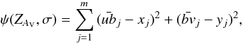
Figure 4 shows the parameter as a function of fractal dimension obtained by LWC11. To illustrate the offset of due to differences in the resolution (or number of points), the clustering statistics for fractal distributions (D = 2.0–3.0) of artificial data is displayed for two data set with N = 1024 points and N = 65 536 points. For comparison with our results, the hatched area in Fig. 4 represents the error bars corresponding to the lower resolution data set.
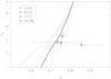 |
Fig. 4 Comparison of our clusters with the |
Despite the low number of members studied in our clusters, their distribution are consistent with the LWC11 set of N = 1024 points, except for NGC 6530, which appears to be displaced away from the cloud-cluster expected correlation.
Cartwright & Whitworth (2004) suggested that clusters with centrally concentrated distributions have that increases from 0.8 to 1.5. On the other hand, clusters with fractal substructures have that decreases from 0.8 to 0.45 related to a fractal dimension decreasing from D2 = 2 to D2 = 0.5 (where we use the same relation between 2D images and 3D distributions adopted above). In fact, NGC 6530 is the only cluster in our sample that has a radial distribution of stars ( ), which is incompatible with the fractal structure of its projected cloud (D2 ~ 1.3). The other clusters members follow a distribution with fractal sub-clustering structure, as indicated by their that agrees with the fractal dimension measured in the respective projected clouds.
Several works have statistically proven that a correlation exists between fractal dimension, which is estimated from cloud maps, and parameter, measured from cluster star distributions. For instance, Camargo et al. (2011) summarises the concepts first discussed by Lada & Lada (2003) suggesting that the structure of embedded clusters is related to the structure of their original molecular cloud. Fractal structures are observed in clouds that have multiple peaks in their density profile (Cartwright & Whitworth 2004; Schmeja et al. 2008; Sánchez et al. 2010, LWC11).
On the basis of our comparison with artificial data, we suggest that for our clusters there is a correlation between the fractal statistics of the cloud and the distribution of cluster members, except for NGC 6530. In this case, the measured fractal dimension does not indicate a uniform density distribution in the cloud, which is expected for associated clusters with centrally concentrated distributions. For this reason, our fractal analysis indicates that NGC 6530 can be described by a different scenario of formation than the other three clusters. Our argument for discussing the cluster formation comes from the interpretation of the cloud-cluster relation, which is derived from the fractal analysis. The meaning of this relation is the comparison of the physical structure of the cluster with its remnant progenitor cloud. In this way, the cloud-cluster relation may tell us about the original gas distribution of the cloud that formed the cluster. It also may give us information on how that particular cloud has probably evolved since forming the cluster.
The concentrated distribution of NGC 6530 indicates that the original material was more concentrated than the fractal structure of the cloud that remained behind the cluster. This material was possibly contained in a massive dense core within the cloud, whose structure was changed by the process of cluster formation consuming the core. This scenario is consistent with the suggestion that NGC 6530 lies within an HII cavity (McCall et al. 1990).
6. Discussion and conclusions
We have developed a detailed study of the extinction in the direction of four clusters with ages < 5 Myr, located in star-forming regions. Our aim has been to search for variable or anomalous extinction that possibly occurs for objects associated to dark clouds. To verify the characteristics of the clouds that coincide with the projected position of the cluster, we inspected the visual extinction maps and compared them to the far-IR emission detected in the direction of our sample.
We used different methods to improve on the previous results on the extinction law RV, providing a means of identifying the cause of anomalous extinction. In this comparative study, we used the same photometric database, ensuring similar observational conditions for the entire sample. Theoretical expressions for the extinction law were adopted to evaluate RV based on the colour-excess E(B − V), which could be determined for some of the cluster members that have spectral types available in the literature. A variable extinction law was clearly verified for NGC 2264, which followed a bimodal distribution. Part of the cluster suffers normal extinction and another part shows a large dispersion in its RV values, as illustrated in Fig. 3. However, these results are inconclusive since few objects of our sample have known spectral types, particularly in Berkeley 86.
A more efficient analysis to estimate RV and its dependence on wavelength was based on TCDs. The slope of the observed colour distribution relative to the slope of ZAMS colours in Table 2 enabled us to infer anomalous extinction for NGC 6530, for which RV = 4.5 is measured in the I band, and RV = 6.2 in K band. The other clusters have on average normal extinction. However, some members of NGC 2264 and NGC 2244 appear to be dispersed in the TCDs, indicating individual anomalous RV, as illustrated in Figs. A.1 and A.2. The TCD analysis confirms the results obtained from the colour-excess analysis, based on spectral type. Since there is no relation between the variation in RV and the spatial distribution of the cluster members, we conclude that differences in the extinction law verified for some cluster members are not caused by environmental differences, but are probably due to circumstellar effects. This agrees particularly with the results of Alencar et al. (2010) confirming for instance, the accretion activity in circumstellar discs of NGC 2264 members.
To confirm whether our results provide a reliable reddening correction, the RV estimated from TCDs was used to determine the visual extinction that most closely fits the observed colours of the cluster members. A ZAMS fitting algorithm was developed to improve the search for AV that minimises the distance of the colour distribution to the reddened ZAMS curve, which was reproduced by spline interpolation. The best-fit provided a mean value for E(B − V), which was compared to the results from other methods (Table 3). All the colour-excess estimates are in good agreement, except for the E(B − V) derived from AV maps mainly for NGC 2264 and NGC 6530. These clusters are not embedded in their respective clouds, which is consistent with the extinction levels found for the cluster members being lower than that measured in the extinction maps for the background stars.
A fractal analysis was performed to investigate the substructures of the clouds and to compare them with the statistical parameters of the cluster member distribution. Our estimate of the parameter indicated that NGC 6530 has a radially clustered spatial distribution, while the other clusters have a fractally sub-clustered distribution of members. The fractal dimension (D2) measured in the AV maps, which is related to the cloud geometry, was compared to measured in the cluster distributions. Except for NGC 6530, the clusters have a parameter that is compatible with the fractal dimension of the corresponding clouds, and in turn similar to the distribution of artificial data. We interpreted this result as a correlation between the cloud structure and the cluster member distribution, which is similar for Berkeley 86, NGC 2244, and NGC 2264. However, NGC 6530 does not follow this cloud-cluster relation, indicating that it was formed from a more centrally concentrated gas distribution that differs of the fractal substructures found in the remaining cloud.
Even for an anomalous RV = 4.5, NGC 6530 does not suffer high extinction based on the average colour-excess (AV ~ 1 mag), which is incompatible with the high levels of extinction shown in either the dark cloud map or the far-IR emission maps. We conclude that the anomalous extinction in this case is not due to interstellar dense regions. A tentative explanation is the depletion of small grains by evaporation that occurs under radiation from hot stars, which is consistent with the location of NGC 6530 in an HII cavity. In addition, the circumstellar effects cannot be disregarded, since the grain growth is expected to occur in protoplanetary discs. In this case, our results also agree with the polarimetric results of McCall et al. (1990), which suggested that the anomalous RV is due to circumstellar effects.
We also verified that the fractal analysis used to investigate the cloud-cluster relation may help us to constrain the scenario of cluster formation. Since the role of this cloud-cluster relation is to compare the physical structure of the cluster with its parental cloud, the interpretation of this relation may tell us about the original gas distribution of the forming cloud and how the particular cloud may have evolved since the cluster was formed. It must be kept in mind that suggesting a cloud-cluster connection based on the correlation of with D2 is only speculative in the case of our sample, since more points would be required to perform a robust analysis. However, we detected a trend when comparing calculations performed for data sets of unrelated origins. This trend implies that the stellar clustering is related to the substructures of the clouds, in a comparable way to the LWC11 findings for artificial clouds and their derived clusters. For this reason, we conclude that NGC 6530 is systematically different from the other clusters, which agrees with previous results from the literature.
It will be interesting to extend our study to a larger number of clusters, particularly those that have not yet been studied in as much detail as our sample has been.
Online material
Appendix A: Colour diagrams
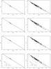 |
Fig. A.1 TCDs for the clusters Berkeley 86 (left) and NGC 2244 (right). The solid line shows a normal extinction law, while the fitting for the cluster members is shown by a dotted line. Two extinction vectors (AV = 2 mag) related to different values of RV are plotted in the bottom panels, for illustration. Open circles indicate the members and crosses show the stars with P% < Pmin. |
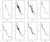 |
Fig. A.3 Top: reddened ZAMS fitting to the cluster members with P% > Pmin (open circles). The position of the other stars of the sample is indicated by crosses. A full line shows the curve obtained with the fitting algorithm, while the dotted line shows the intrinsic U − B and B − V colours. Bottom: curves representing the limit ΔE(B − V) = 0.11 suggested by Burki (1975). From left to right: Berkeley 86, NGC 2244, NGC 2264, and NGC 6530. |
Acknowledgments
Part of this work was supported by CAPES/Cofecub Project 712/2011. B.F. thanks CNPq Project 142849/2010-3. This publication makes use of data products from the Two Micron All Sky Survey, which is a joint project of the University of Massachusetts and the Infrared Processing and Analysis Center/California Institute of Technology, funded by the National Aeronautics and Space Administration and the National Science Foundation.
References
- Alencar, S. P. H., Bouvier, J., Catala, C., et al. 2010, in Highlights of Astrophysics, 15, 735 [Google Scholar]
- Amôres, E. B., & Lépine, J. R. D. 2005, AJ, 130, 659 [NASA ADS] [CrossRef] [Google Scholar]
- Arias, J. I., Barbá, R. H., & Morrell, N. I. 2007, MNRAS, 374, 1253 [NASA ADS] [CrossRef] [Google Scholar]
- Bhavya, B., Mathew, B., & Subramaniam, A. 2007, Bull. Astr. Soc. India, 35, 383 [NASA ADS] [Google Scholar]
- Bessell, M. S., Castelli, F., & Plez, B. 1998, A&A, 333, 231 [NASA ADS] [Google Scholar]
- Burki, G. 1975, A&A, 43, 37 [NASA ADS] [Google Scholar]
- Camargo, D., Bonatto, C., & Bica, E. 2011, MNRAS, 416, 1522 [NASA ADS] [CrossRef] [Google Scholar]
- Cambrésy, L., Rho, J., Marshall, D. J., & Reach, W. T. 2011, A&A, 527, A141 [NASA ADS] [CrossRef] [EDP Sciences] [Google Scholar]
- Cardelli, J. A., Clayton, G. C., & Mathis, J. S. 1989, ApJ, 345, 245 [NASA ADS] [CrossRef] [Google Scholar]
- Cartwright, A., & Whitworth, A. P. 2004, MNRAS, 348, 589 [NASA ADS] [CrossRef] [Google Scholar]
- Chauhan, N., Pandey, A. K., Ogura, K., et al. 2011, MNRAS 415, 1202 [Google Scholar]
- Chini, R., & Krugel, E. 1983, A&A, 117, 289 [NASA ADS] [Google Scholar]
- Chini, R., & Wargau, W. F. 1990, A&A, 227, 213 [NASA ADS] [Google Scholar]
- Conti, P. S., & Leep, E. M. 1974, ApJ, 193, 113 [NASA ADS] [CrossRef] [Google Scholar]
- Cutri, R. M. 2003, The Two Micron All Sky Survey at IPAC (2MASS), California Institute of Technology [Google Scholar]
- DaRio, N., Robberto, M., Soderblom, D. R., et al. 2010, ApJ, 722, 1092 [NASA ADS] [CrossRef] [Google Scholar]
- Dahm, S. E. 2008, Handbook of Star Forming Regions Vol. I, 966 [Google Scholar]
- Deeg, H. J., & Ninkov, Z. 1996, A&AS, 119, 221 [NASA ADS] [CrossRef] [EDP Sciences] [Google Scholar]
- Dias, W. S., Lépine, J. R. D., & Alessi, B. S. 2002a, A&A, 388, 168 [Google Scholar]
- Dias, W. S., Alessi, B. S., Moitinho, A., & Lépine, J. R. D. 2002b, A&A, 389, 871 [NASA ADS] [CrossRef] [EDP Sciences] [Google Scholar]
- Dias, W. S., Assafin, M., Flório, V., Alessi, B. S., & Líbero, V. 2006, A&A, 446, 949 [NASA ADS] [CrossRef] [EDP Sciences] [Google Scholar]
- Dobashi, K., Uehara, H., Kandori, R., et al. 2005, PASJ, 57, 1 [Google Scholar]
- Eswaraiah, C., Pandey, A. K., Maheswar, G., et al. 2012, MNRAS, 419, 2587 [NASA ADS] [CrossRef] [Google Scholar]
- Elmegreen, B. G. 2010, in Star Clusters: basic galactic building blocks, Proc. IAU Symp., 266, 2009, ed. R. de Grijs, & J. R. D. Lépine, 3 [Google Scholar]
- Fitzpatrick, E. L., & Massa, D. 2009, ApJ, 699, 1209 [NASA ADS] [CrossRef] [Google Scholar]
- Flaccomio, E., Sciortino, S., Micela, G., et al. 1997, Mem. Soc. Astron. Ital., 68, 1073 [Google Scholar]
- Forbes, D. 1981, PASPS, 93, 441 [NASA ADS] [CrossRef] [Google Scholar]
- Forbes, D., English, D., De Robertis, M. M., & Dawson, P. C. 1992, AJ, 103, 916 [NASA ADS] [CrossRef] [Google Scholar]
- Gregorio-Hetem, J. C., Sanzovo, G. C., & Lépine, J. R. D. 1988, A&AS, 76, 347 [NASA ADS] [Google Scholar]
- Guetter, H. H., & Vrba, F. J. 1989, AJ, 98, 611 [NASA ADS] [CrossRef] [Google Scholar]
- Hoag, A. A., & Smith, E. V. P. 1959, PASP, 71, 32 [NASA ADS] [CrossRef] [Google Scholar]
- de Jager, C., & Nieuwenhuijzen, H. 1987, A&A, 177, 217 [NASA ADS] [Google Scholar]
- Johnson, H. L. 1962, ApJ, 136, 1135 [NASA ADS] [CrossRef] [Google Scholar]
- Johnson, H. L. 1968, in Interstellar Extinction, Nebulae and Interstellar Matter. Library of Congress Catalog Card Number 66-13879, ed. B. M. Middlehurst, & L. H. Aller (Chicago, IL: Univ. of Chicago Press), 167 [Google Scholar]
- Jose, J., Pandey, A. K., Ojha, D. K., et al. 2008, MNRAS, 384, 1675 [NASA ADS] [CrossRef] [Google Scholar]
- Jose, J., Pandey, A. K., Ogura, K., et al. 2011, MNRAS, 411, 2530 [NASA ADS] [CrossRef] [Google Scholar]
- Hetem, A., & Lépine, J. R. D. 1993, A&A 270, 451 [NASA ADS] [CrossRef] [Google Scholar]
- Hillenbrand, L. A., Massey, P., Strom, S. E., & Merrill, K. M. 1993, AJ, 106, 1906 [NASA ADS] [CrossRef] [Google Scholar]
- Hiltner, W. A., Morgan, W. W., & Neff, J. S. 1965, ApJ, 141, 183 [NASA ADS] [CrossRef] [Google Scholar]
- Kruskal, J. B. J. 1956, Proc. Amer. Math. Soc., 7, 48 [CrossRef] [MathSciNet] [Google Scholar]
- Lada, C. J., & Lada, E. A. 2003, ARA&A, 41, 57 [NASA ADS] [CrossRef] [Google Scholar]
- Lomax, O., Whitworth, P., & Cartwright, A. 2011, MNRAS, 412, 627 [NASA ADS] [CrossRef] [Google Scholar]
- Mandelbrot, B. B. 1983, The Fractal Geometry of Nature (New York: W.H. Freeman and Co.) [Google Scholar]
- Mayne, N. J., & Naylor, T. 2008, MNRAS, 386, 261 [NASA ADS] [CrossRef] [Google Scholar]
- McCall, M. L., Richer, G. M., & Visvanathan, N. 1990, ApJ, 357, 502 [NASA ADS] [CrossRef] [Google Scholar]
- Megiddo, N. 1983, SIAM J. Comput., 12, 759 [CrossRef] [Google Scholar]
- Melena, N. W., Massey, P., Morrell, N. I., & Zangari, A. M. 2008, AJ, 135, 878 [NASA ADS] [CrossRef] [Google Scholar]
- Monteiro, H., & Dias, W. S. 2011, A&A, 530, A91 [NASA ADS] [CrossRef] [EDP Sciences] [Google Scholar]
- Monteiro, H., Dias, W. S., & Caetano, T. C. 2010 A&A, 516, A2 [Google Scholar]
- Morgan, W. W., Hiltner, W. A., Neff, J. S., Garrison, R., & Osterbrock, D. E. 1965, ApJ, 142, 974 [NASA ADS] [CrossRef] [Google Scholar]
- Neckel, T., & Chini, R. 1981, A&AS, 45, 451 [NASA ADS] [Google Scholar]
- Ogura, K., & Ishida, K. 1981, PASJ, 33, 149 [NASA ADS] [Google Scholar]
- Pandey, A. K., Ogura, K., & Sekiguchi, K. 2000, PASJ, 52, 847 [NASA ADS] [CrossRef] [Google Scholar]
- Park, B.-G., & Sung, H. 2002, AJ, 123, 892 [NASA ADS] [CrossRef] [Google Scholar]
- Pérez, M. R., Thé, P. S., & Westerlund, B. E. 1987, PASP, 99, 1050 [NASA ADS] [CrossRef] [Google Scholar]
- Press, W., Teukolsky, S., Vetterling, W., & Flannery, B. 1995, Numerical Recipes in C 2nd edn. (Cambridge, UK: Cambridge University Press) [Google Scholar]
- Prisinzano, L., Sanz-Forcada, J., Micela, G., et al. 2011, A&A, 527, A77 [NASA ADS] [CrossRef] [EDP Sciences] [Google Scholar]
- Rebull, L. M., Makifon, R. B., Strom, S. E., et al. 2002, AJ, 123, 1528 [NASA ADS] [CrossRef] [Google Scholar]
- Reipurth, B., & Schneider, N. 2008, Handbook of Star Forming Regions Vol. I, 36 [Google Scholar]
- Róman-Zúñiga, C. G., & Lada, E. A. 2008, Handbook of Star Forming Regions Vol. I, 929 [Google Scholar]
- Samal, M. R., Pandey, A. K., Ojha, D. K., et al. 2007, ApJ, 671, 555 [NASA ADS] [CrossRef] [Google Scholar]
- Sánchez, N., & Alfaro, E. J. 2010, Lect. Notes Essays Astrophys., 4, 1 [Google Scholar]
- Sánchez, N., Alfaro, E. J., & Pérez, E. 2005, ApJ, 625, 849 [NASA ADS] [CrossRef] [Google Scholar]
- Sanduleak, N. 1974, PASP, 86, 74 [NASA ADS] [CrossRef] [Google Scholar]
- Savage, B. D., & Mathis, J. S. 1979, ARA&A, 17, 73 [NASA ADS] [CrossRef] [Google Scholar]
- Schlegel, D. J., Finkbeiner, D. P., & Davis, M. 1998, ApJ, 500, 525 [NASA ADS] [CrossRef] [Google Scholar]
- Schmeja, S., Kumar, M. S. N., & Ferreira, B. 2008, MNRAS, 389, 1209 [NASA ADS] [CrossRef] [Google Scholar]
- Setteducati, A. F., & Weaver, H. F. 1962, Berkeley: Radio Astronomy Laboratory, 474, 873 [Google Scholar]
- Siess, L., Dufour, E., & Forestini, M. 2000, A&A, 358, 593 [NASA ADS] [Google Scholar]
- Steenman, H., & Thé, P. S. 1991, Ap&SS, 184, 9 [NASA ADS] [CrossRef] [Google Scholar]
- Straizys, V., & Kuriliene, G. 1981, Ap&SS, 80, 353 [NASA ADS] [CrossRef] [Google Scholar]
- Sung, H., Bessell, M. S., & Lee, S.-W. 1997, AJ, 114, 2644 [NASA ADS] [CrossRef] [Google Scholar]
- Sung, H., Chun, M.-Y., & Bessell, M. S. 2000, AJ, 120, 333 [NASA ADS] [CrossRef] [Google Scholar]
- Tothill, N. F. H., Gagné, M., Stecklum, B., & Kenworthy, M. A. 2008, Handbook of Star Forming Regions Vol. II, 533 [Google Scholar]
- Turcotte, D. 1997, Fractals and Chaos in Geology and Geophysics (Cambridge: Cambridge University Press), 398 [Google Scholar]
- Turner, D. G. 1976, ApJ, 210, 65 [NASA ADS] [CrossRef] [Google Scholar]
- van den Ancker, M. E., Thé, P. S., Feinstein, A., et al. 1997, A&AS, 123, 63 [NASA ADS] [CrossRef] [EDP Sciences] [Google Scholar]
- Walker, M. F. 1954, AJ, 59, 333 [CrossRef] [Google Scholar]
- Walker, M. F. 1956, ApJS, 2, 365 [NASA ADS] [CrossRef] [Google Scholar]
- Wang, J., Townsley, L. K., Feigelson, E. D., et al. 2008, ApJ, 675, 464 [NASA ADS] [CrossRef] [Google Scholar]
- Welsh, B. Y. 1983, MNRAS, 204, 1203 [NASA ADS] [Google Scholar]
- Wolff, S. C., Strom, S. E., Dror, D., & Venn, K. 2007, AJ, 133, 1092 [NASA ADS] [CrossRef] [Google Scholar]
- Yadav, R. K. S., & Sagar, R. 2001, MNRAS, 328, 370 [NASA ADS] [CrossRef] [Google Scholar]
- Young, A. 1978, PASP, 90, 144 [NASA ADS] [CrossRef] [Google Scholar]
All Tables
All Figures
|
Fig. 1 Normalised number of stars distributed according to membership probability (P%), which is based on their proper motion. A dotted line indicates the minimum probability (Pmin) that was adopted to separate the most probable members from field stars. Top: Berkeley 86 (left) and NGC 2244 (right). Bottom: NGC 2264 (left) e NGC 6530 (right). |
| In the text | |
|
Fig. 2 Map of visual extinction over-imposed by contours measured from IRIS-IRAS images at 100 μm band. The contours vary from 50–350 MJy/Sr with steps of 100 MJy/Sr, except for NGC 6530 that has contours starting at 500 MJy/Sr with steps of 1000 MJy/Sr. The area of the cluster is indicated by the black central square. |
| In the text | |
|
Fig. 3 Different extinction laws compared to the colour-excess distribution for cluster members with available spectral types. Error bars illustrate the maximum uncertainty expected, if the spectral type is not well-determined, for a G8 star. |
| In the text | |
|
Fig. 4 Comparison of our clusters with the |
| In the text | |
|
Fig. A.1 TCDs for the clusters Berkeley 86 (left) and NGC 2244 (right). The solid line shows a normal extinction law, while the fitting for the cluster members is shown by a dotted line. Two extinction vectors (AV = 2 mag) related to different values of RV are plotted in the bottom panels, for illustration. Open circles indicate the members and crosses show the stars with P% < Pmin. |
| In the text | |
|
Fig. A.3 Top: reddened ZAMS fitting to the cluster members with P% > Pmin (open circles). The position of the other stars of the sample is indicated by crosses. A full line shows the curve obtained with the fitting algorithm, while the dotted line shows the intrinsic U − B and B − V colours. Bottom: curves representing the limit ΔE(B − V) = 0.11 suggested by Burki (1975). From left to right: Berkeley 86, NGC 2244, NGC 2264, and NGC 6530. |
| In the text | |
Current usage metrics show cumulative count of Article Views (full-text article views including HTML views, PDF and ePub downloads, according to the available data) and Abstracts Views on Vision4Press platform.
Data correspond to usage on the plateform after 2015. The current usage metrics is available 48-96 hours after online publication and is updated daily on week days.
Initial download of the metrics may take a while.