| Issue |
A&A
Volume 541, May 2012
|
|
|---|---|---|
| Article Number | A46 | |
| Number of page(s) | 11 | |
| Section | Astronomical instrumentation | |
| DOI | https://doi.org/10.1051/0004-6361/201117335 | |
| Published online | 26 April 2012 | |
Detection noise bias and variance in the power spectrum and bispectrum in optical interferometry
Astrophysics Group, Cavendish Laboratory, University of
Cambridge, J.J. Thomson
Avenue, Cambridge
CB3 0HE, UK
e-mail: This email address is being protected from spambots. You need JavaScript enabled to view it.
Received:
24
May
2011
Accepted:
12
March
2012
Abstract
Context. Long-baseline optical interferometry uses the power spectrum and bispectrum constructs as fundamental observables. Noise arising in the detection of the fringe pattern results in both variance and biases in the power spectrum and bispectrum. Previous work on correcting the biases and estimating the variances for these quantities typically includes restrictive assumptions about the sampling of the interferogram and/or about the relative importance of Poisson and Gaussian noise sources. Until now it has been difficult to accurately compensate for systematic biases in data which violates these assumptions.
Aims. We seek a formalism to allow the construction of bias-free estimators of the bispectrum and power spectrum, and to estimate their variances, under less restrictive conditions, which include both unevenly-sampled data and measurements affected by a combination of noise sources with Poisson and Gaussian statistics.
Methods. We used a method based on the moments of the noise distributions to derive formulae for the biases introduced to the power spectrum and bispectrum when the complex fringe amplitude is derived from an arbitrary linear combination of a set of discrete interferogram measurements.
Results. We have derived formulae for bias-free estimators of the power spectrum and bispectrum, which can be used with any linear estimator of the fringe complex amplitude. We have demonstrated the importance of bias-free estimators for the case of the detection of faint companions (for example exoplanets) using closure phase nulling. We have derived formulae for the variance of the power spectrum and have shown how the variance of the bispectrum can be calculated.
Key words: instrumentation: interferometers / techniques: interferometric / methods: analytical
© ESO, 2012
1. Introduction
Astronomical interferometers combine the light from multiple telescopes to form interference fringes. The amplitude and phase of the fringes corresponding to interference between a given pair of telescopes can be combined into a single complex number, the fringe complex amplitude, which in an ideal interferometer is proportional to a single Fourier component of the object brightness distribution.
The complex amplitude forms the fundamental observable in phase-stable interferometric experiments, for example at radio wavelengths, but at optical wavelengths the phase of the fringes is unstable on timescales of order milliseconds, because of optical pathlength perturbations introduced by the Earth’s atmosphere. As a result, observers need to combine the information from multiple short-exposure interferograms to recover the desired science data. Since the phase of the fringes is randomly fluctuating, simply averaging the complex amplitude over multiple interferograms would lead to a vanishingly small result. Instead two observables, the power spectrum and bispectrum, are calculated from each interferogram and these can be averaged over frames as both are immune (to first order) to the atmospheric and instrumental phase perturbations. The power spectrum serves to capture information about the modulus of the complex amplitude, whilst the phase of the bispectrum (also known as the “closure phase”) captures information about the phase of the complex amplitude on closed triplets of baselines.
At the low light levels typically encountered in astronomical interferometry, the effects of the noise arising in the detection process become important. This noise can usually be modelled as a mixture of Poisson noise, for example photon noise, and signal-independent Gaussian noise, for example readout noise in the detector electronics. We use the term “detection noise” to refer to the combination of all the noise processes in the detection process including the photon noise.
Detection noise produces random measurement errors which can be reduced by averaging over many interferograms, but in the case of the power spectrum and bispectrum it also produces systematic biases in the averaged estimates. There has been considerable study in the literature on these biases (see for example Goodman & Belsher 1976a,b; Sibille et al. 1979; Wirnitzer 1985; Beletic 1989; Perrin 2003). Some authors have derived formulae for the power spectrum bias which allow for both Poisson and Gaussian noise sources, but existing bispectrum bias estimates have been derived under the assumption of Poisson noise only. As a result, it is difficult to derive an unbiased estimate of the closure phase from observations where both Poisson and Gaussian noise are significant. Such conditions are increasingly present in interferometric observations made at near-infrared wavelengths so the absence of such an estimator is becoming a critical limitation to the acquisition of accurate interferometric data as we will demonstrate in Sect. 8.
Much of the existing power spectrum and bispectrum analysis relies on the direct Fourier transform of the interferogram to recover the fringe complex amplitudes. Even under noise-free conditions the use of a Fourier-based estimator will return inaccurate estimates of the fringe complex amplitude if the interferogram is, for example, non-uniformly sampled. To account for this, Tatulli & Le Bouquin (2006) introduced a pixel-to-visibility transformation matrix (P2VM) for deriving fringe amplitude estimates in circumstances where the Fourier-based estimators are inaccurate, which includes the Fourier estimators as a special case.
There has been considerable study of the variance of the power spectrum and bispectrum (Goodman & Belsher 1976a,b; Dainty & Greenaway 1979; Sibille et al. 1979; Wirnitzer 1985; Roddier 1987; Ayers et al. 1988), but only the work of Tatulli & Le Bouquin (2006) applies the more general P2VM approach, and in this case the variance is calculated under assumptions valid only for purely Gaussian noise processes. Knowing the variance, and hence the signal-to-noise ratio is important for predicting the integration times and detection limits prior to an observation run.
This paper builds on the introduction by Gordon et al. (2010) and previous work by Thorsteinsson & Buscher (2004) to present a general formalism for computing biases and variances in the presence of detection noise. Our formalism has two advantages over current treatments: (a) it can be applied when the fringe complex amplitudes are derived using any linear estimator, including the P2VM and Fourier transform as special cases and (b) it yields accurate answers for any additive mixture of Poisson noise and Gaussian noise. We derive formulae for the biases affecting both the power spectrum and bispectrum under these conditions and show how our results allow the construction of bias-free estimators. We present simulations to show that using our new bispectrum estimator can significantly enhance the accuracy of measuring the closure phase under realistic observation conditions. We also use our formalism to derive expressions for the variance of the power spectrum, and explain the method by which the reader can calculate the bispectrum variance if required.
2. The interferometric equations
2.1. The interferogram
We will start from a specific idealised example and use this to introduce our more
general model which will be applicable to a wide range of realistic scenarios. In our
example, the light from Ntel telescopes is combined to produce
a 1-dimensional interference pattern, which consists of the superposition of a set of
sinusoidal fringes at different fringe frequencies
fij corresponding to the interference
between telescopes i and j. The interference pattern is
sampled to produce a set of Npix intensity measurements
{ip} . We shall call this discrete set of
intensity measurements the “interferogram”. In our example the interferogram is given by:
![Mathematical equation: \begin{equation} \label{eq:simplesample} i_p=\frac{C^{00}}{N_{\rm pix}}+ \frac{1}{N_{\rm pix}}\sum_{i<j}^{N_{\rm tel}}\mathrm{Re}\left[ C^{ij}{\rm e}^{2\pi{\rm i}\alpha_{p}f^{ij}} \right] +{\rm noise}, \end{equation}](/articles/aa/full_html/2012/05/aa17335-11/aa17335-11-eq7.png) (1)where
Cij denotes the complex amplitude of the
fringes corresponding to interference between light from telescopes i and
j, C00 denotes an offset due to the light
from all the telescopes (we shall call this the “zero-spacing flux”), and
αp is the coordinate of pixel
p.
(1)where
Cij denotes the complex amplitude of the
fringes corresponding to interference between light from telescopes i and
j, C00 denotes an offset due to the light
from all the telescopes (we shall call this the “zero-spacing flux”), and
αp is the coordinate of pixel
p.
Recognising that Eq. (1) represents a sum
over a set of Fourier components, we can derive an estimate
cij of the complex amplitudes from the
sampled intensity data using a discrete Fourier transform (DFT):  (2)where we note that this equation can also be
used to estimate the zero-spacing flux by setting f00 = 0. In
noise-free conditions, the estimator cij will
be equal to the true amplitudes Cij provided
that the samples are evenly spaced in the coordinate α and the
frequencies fij are integer multiples of the
fundamental frequency given by
ffundamental = 1/ [Npix(α2 − α1)] .
We will call this set of conditions the “DFT conditions”.
(2)where we note that this equation can also be
used to estimate the zero-spacing flux by setting f00 = 0. In
noise-free conditions, the estimator cij will
be equal to the true amplitudes Cij provided
that the samples are evenly spaced in the coordinate α and the
frequencies fij are integer multiples of the
fundamental frequency given by
ffundamental = 1/ [Npix(α2 − α1)] .
We will call this set of conditions the “DFT conditions”.
We can rewrite the above equations in the form:  (3)and:
  (4)respectively where
i = [i1,i2,...]
is a vector containing the pixel intensities,
C = [C00,
Re {C12}, Im {C12},
Re {C13}, Im {C13},
...] is a vector describing the true complex amplitudes,
c = [c00,Re {c12},
Im {c12}, Re {c13},
Im {c13}, ...] is a vector describing the
estimated complex amplitudes, W is a matrix known as the
“visibility-to-pixel matrix” (V2PM) and H is the
pixel-to-visibility matrix (P2VM) mentioned before. When the DFT conditions hold, the
matrices W and H will consist
of sine and cosine terms.
(4)respectively where
i = [i1,i2,...]
is a vector containing the pixel intensities,
C = [C00,
Re {C12}, Im {C12},
Re {C13}, Im {C13},
...] is a vector describing the true complex amplitudes,
c = [c00,Re {c12},
Im {c12}, Re {c13},
Im {c13}, ...] is a vector describing the
estimated complex amplitudes, W is a matrix known as the
“visibility-to-pixel matrix” (V2PM) and H is the
pixel-to-visibility matrix (P2VM) mentioned before. When the DFT conditions hold, the
matrices W and H will consist
of sine and cosine terms.
If we now assume that the DFT conditions do not hold, for example if the samples are not
evenly spaced or there are “dead” pixels, then it is often still possible to set up a
linear set of equations in the form of Eq. (3) by modifying the matrix W. For the case of any “working”
beam combiner, we can always find the corresponding matrix H such that:
 (5)where I is the
identity matrix, i.e. Eq. (5) is the
condition that H is a pseudo-inverse of
W. It is then clear that Eq. (4) can be used to derive a value for
c such that
c = C under noise-free
conditions. The pseudo-inverse generalises the Fourier inverse to the cases in which the
DFT conditions may not hold; in general the pseudo-inverse matrix will not consist of
simple Fourier terms.
(5)where I is the
identity matrix, i.e. Eq. (5) is the
condition that H is a pseudo-inverse of
W. It is then clear that Eq. (4) can be used to derive a value for
c such that
c = C under noise-free
conditions. The pseudo-inverse generalises the Fourier inverse to the cases in which the
DFT conditions may not hold; in general the pseudo-inverse matrix will not consist of
simple Fourier terms.
Equation (4) serves to define the basis of
our more general model for an interferometric measurement. We assume only a discrete set
of intensity measurements {ip} related to a
set of complex fringe amplitudes {Cij} . We
do not require a simple Fourier relationship between the amplitudes and the pixel
intensities; we only require that there exists a set of estimators for
{Cij} which are linear in
{ip} . In other words we require only that
there exists at least one set of complex weights  such that the complex amplitude
estimators:
such that the complex amplitude
estimators:  (6)have the property that
cij = Cij
in the limit where detection noise can be neglected. This generalised model can be applied
to a wide variety of beam combination scenarios: the interferograms can be sampled
temporally or spatially or a combination of the two, and multiple telescopes can be
combined “all-in-one” into a single multiplexed fringe pattern or pairwise onto separate
detectors.
(6)have the property that
cij = Cij
in the limit where detection noise can be neglected. This generalised model can be applied
to a wide variety of beam combination scenarios: the interferograms can be sampled
temporally or spatially or a combination of the two, and multiple telescopes can be
combined “all-in-one” into a single multiplexed fringe pattern or pairwise onto separate
detectors.
Note that pseudo-inverse techniques are only presented as one possible route to deriving
 ; under circumstances where the forward
matrix W is not known or not fixed (for example if the fringe pattern has
not been spatially filtered) alternative techniques to derive
, perhaps based on knowing the statistical
properties of W, may be needed. Nevertheless, the results presented here
will be valid independent of the technique used to derive values for
; under circumstances where the forward
matrix W is not known or not fixed (for example if the fringe pattern has
not been spatially filtered) alternative techniques to derive
, perhaps based on knowing the statistical
properties of W, may be needed. Nevertheless, the results presented here
will be valid independent of the technique used to derive values for
 .
.
2.2. Interferometric observables
Under phase-unstable conditions, it is common to choose the power spectrum,
Sij and bispectrum,
Bijk as the interferometric observables:
 (7)and:
  (8)Typically the values of
Cij will change randomly from
interferogram to interferogram due to atmospheric disturbances, but the values of
Sij and
Bijk will be more stable. However, unless
otherwise specified, we do not assume any particular distribution for the values of
Cij; for example the results will apply
equally well under incoherent conditions where the average value of
Cij is zero or conditions where a fringe
tracker is being used and the value of Cij is
stable from frame to frame. Our aim is to determine suitable estimators,
(8)Typically the values of
Cij will change randomly from
interferogram to interferogram due to atmospheric disturbances, but the values of
Sij and
Bijk will be more stable. However, unless
otherwise specified, we do not assume any particular distribution for the values of
Cij; for example the results will apply
equally well under incoherent conditions where the average value of
Cij is zero or conditions where a fringe
tracker is being used and the value of Cij is
stable from frame to frame. Our aim is to determine suitable estimators,
 ,
,  , for the power spectrum and bispectrum
respectively that do not suffer from bias in the presence of noise. For this analysis
these observables are calculated on an interferogram-by-interferogram basis and then
averaged. Derived quantities, such as the closure phase, are calculated using the averaged
observables, rather than on an interferogram-by-interferogram basis themselves.
, for the power spectrum and bispectrum
respectively that do not suffer from bias in the presence of noise. For this analysis
these observables are calculated on an interferogram-by-interferogram basis and then
averaged. Derived quantities, such as the closure phase, are calculated using the averaged
observables, rather than on an interferogram-by-interferogram basis themselves.
3. Noise model
The signal recorded by a real detector system will always have some noise component, which becomes especially important at low light levels. We model two distinct sources of noise, photon shot noise and detector read noise.
3.1. Photon noise
Photon noise is always present in a real interferogram as a result of the quantum nature
of the detection process which converts the incoming photons to an electrical signal. For
a given pixel p, the probability of
Np photoevents occurring is given by the
Poisson distribution: ![Mathematical equation: \begin{equation} P_{\textrm{Poisson}}\left(N_{p}|\Lambda_{p}\right) = \sum_{n}^{\infty}\delta\left(N_{p}-n\right)\frac{\Lambda_{p}^{N_{p}}}{N_{p}!}\exp\left[-\Lambda_{p}\right],\label{eqn:poisson} \end{equation}](/articles/aa/full_html/2012/05/aa17335-11/aa17335-11-eq46.png) (9)where Λp is the
ideal noise-free intensity, also called the “classical intensity” or “high-light-level
intensity”. Note that this equation implicitly defines the normalisation of
Λp in units of photoevents, and we require that
ip = Λp under
noise-free conditions, thereby defining the normalisation of
ip.
(9)where Λp is the
ideal noise-free intensity, also called the “classical intensity” or “high-light-level
intensity”. Note that this equation implicitly defines the normalisation of
Λp in units of photoevents, and we require that
ip = Λp under
noise-free conditions, thereby defining the normalisation of
ip.
3.2. Read noise
Read noise is present in all optical and IR detectors and is often significant at low
light levels. Assuming the read noise is independent of the number of photoevents, the
probability of a given measurement error
ϵp = ip − Np
is given by the Gaussian distribution:
![Mathematical equation: \begin{equation} P_{\textrm{Gaussian}}\left(\epsilon_{p}|\sigma_{p}, N_{p}\right) = \frac{1}{\sqrt{2\pi\sigma_{p}^{2}}}\exp\left[-\frac{\left(\epsilon_{p}\right)^{2}}{2\sigma_{p}^{2}}\right] \end{equation}](/articles/aa/full_html/2012/05/aa17335-11/aa17335-11-eq51.png) (10)where
(10)where  is the variance of the noise on pixel
p; note that the variance is not assumed to be the same on all pixels.
is the variance of the noise on pixel
p; note that the variance is not assumed to be the same on all pixels.
3.3. Other sources of noise
There are additional noise sources that follow the same statistics as photon or read noise. Detector dark current, Dp, for example is also described by the Poisson distribution and could be included in our formalism by replacing Λp with Λp + Dp in Eq. (9). For the sake of readability dark current will not be explicitly included in this paper.
3.4. Combined noise model
If the photon noise and read noise are statistically independent then the probability of
obtaining the noisy data, ip, from the
underlying ideal data, Λp, is given by:
 (11)The combined noise distribution is a
convolution of the Poisson noise and Gaussian noise distributions, so it is convenient to
derive the moments of our noise model via the moment-generating function of the
probability distribution. The moment-generating function for the combined noise model
probability density
(11)The combined noise distribution is a
convolution of the Poisson noise and Gaussian noise distributions, so it is convenient to
derive the moments of our noise model via the moment-generating function of the
probability distribution. The moment-generating function for the combined noise model
probability density  is proportional to the product of the
moment-generating functions MPoisson and
MGaussian of the individual distributions:
is proportional to the product of the
moment-generating functions MPoisson and
MGaussian of the individual distributions:
![Mathematical equation: \begin{equation} M\left(\nu\right) \!=\! M_{\textrm{Poisson}}\left(\nu\right)M_{\textrm{Gaussian}}\left(\nu\right) \!=\! \exp\left[\frac{\sigma_{p}^{2}\nu^{2}}{2}\right]\exp\left[-\Lambda_{p}+\Lambda_{p} \mathrm{e}^{\nu}\right]. \end{equation}](/articles/aa/full_html/2012/05/aa17335-11/aa17335-11-eq61.png) (12)The first four moments of the noise model as
required to derive the results given in this paper are:
(12)The first four moments of the noise model as
required to derive the results given in this paper are:  where ⟨ ... ⟩ denotes
taking the expectation over the probability distribution of the detection noise. For
simplicity, only the statistics of the measured data for fixed
{Λp} is considered at first; averaging over multiple
interferograms will be considered later. As such the angle brackets do not
denote taking an average over the distribution of possible values of
{Λp}, due to, for example, atmospheric distortions to the
interferograms.
where ⟨ ... ⟩ denotes
taking the expectation over the probability distribution of the detection noise. For
simplicity, only the statistics of the measured data for fixed
{Λp} is considered at first; averaging over multiple
interferograms will be considered later. As such the angle brackets do not
denote taking an average over the distribution of possible values of
{Λp}, due to, for example, atmospheric distortions to the
interferograms.
An important assumption of the following analysis is that the detection noise on different pixels is statistically independent so that for example ⟨ ip1ip2 ⟩ = ⟨ ip1 ⟩ ⟨ ip2 ⟩ for p1 ≠ p2. It should be noted that this assumption will not be true in all cases of practical interest. For example when temporally-sampling an interferogram with a near-IR detector, it is common not to reset the charge accumulation capacitors at each pixel between successive time samples, so that a flux measurement ip is derived from the difference between the voltage readings on two successive samples; in this case the final reading for one sample represents the initial reading for the next sample and so the noise on the two samples is correlated. Treating such readout schemes is beyond the scope of the current paper.
4. Bias-free power spectrum estimator
We seek an estimator  for the noise-free power spectrum
Sij that does not suffer from statistical
bias introduced by the noise on the interferogram. A bias-free estimator was calculated by
Tatulli & Duvert (2007) in the presence of
photon noise and read noise, but we present an alternative derivation here to demonstrate
our analysis method. For the purposes of evaluating the power spectrum, we drop all
telescope-pair-dependent superscripts, for example writing
for the noise-free power spectrum
Sij that does not suffer from statistical
bias introduced by the noise on the interferogram. A bias-free estimator was calculated by
Tatulli & Duvert (2007) in the presence of
photon noise and read noise, but we present an alternative derivation here to demonstrate
our analysis method. For the purposes of evaluating the power spectrum, we drop all
telescope-pair-dependent superscripts, for example writing
 as
Hp.
as
Hp.
We start by evaluating the expectation value of the biased estimator
|c|2. Combining Eqs. (6) and (7) we get:  (17)We split the sum in Eq. (17) for the cases where
p1 = p2(≡ p) and for
p1 ≠ p2 which gives:
(17)We split the sum in Eq. (17) for the cases where
p1 = p2(≡ p) and for
p1 ≠ p2 which gives:
 (18)noting that
⟨ ip1ip2 ⟩ = ⟨ ip1 ⟩ ⟨ ip2 ⟩
for p1 ≠ p2. Substitution of the moments of the noise
model given in Eqs. (13) and (14) leads to:
(18)noting that
⟨ ip1ip2 ⟩ = ⟨ ip1 ⟩ ⟨ ip2 ⟩
for p1 ≠ p2. Substitution of the moments of the noise
model given in Eqs. (13) and (14) leads to:  (19)The noise-free power spectrum,
S, can be expressed in terms of the noise-free interferogram,
Λp, as:
(19)The noise-free power spectrum,
S, can be expressed in terms of the noise-free interferogram,
Λp, as:  (20)this can be split into terms equivalent to
those in Eq. (19):
(20)this can be split into terms equivalent to
those in Eq. (19):  (21)which can be substituted into Eq. (19) to give:
 (22)and written in terms of the noisy
interferograms we see:
(22)and written in terms of the noisy
interferograms we see:  (23)The bias-free power spectrum estimator,
S0, is then:
(23)The bias-free power spectrum estimator,
S0, is then:  (24)It needs to be remembered that
S0 is intended to be evaluated on a per-interferogram,
i.e. frame-by-frame basis as atmospheric turbulence changes the shape of the interferogram
between frames. It is straightforward to show that when this estimator is averaged over a
number of frames that the average is itself unbiased. This is because taking the average
over frames commutes with taking the expectation over the detection statistics, so that:
(24)It needs to be remembered that
S0 is intended to be evaluated on a per-interferogram,
i.e. frame-by-frame basis as atmospheric turbulence changes the shape of the interferogram
between frames. It is straightforward to show that when this estimator is averaged over a
number of frames that the average is itself unbiased. This is because taking the average
over frames commutes with taking the expectation over the detection statistics, so that:
 (25)where
Nf denotes the number of frames over which
the average is taken. This result depends on the assumption that the detection noise is
dependent only on the value of the flux Λp in each pixel and is
statistically independent of the particular shape of the interferogram and hence of the
atmospheric distortions affecting a particular interferogram.
(25)where
Nf denotes the number of frames over which
the average is taken. This result depends on the assumption that the detection noise is
dependent only on the value of the flux Λp in each pixel and is
statistically independent of the particular shape of the interferogram and hence of the
atmospheric distortions affecting a particular interferogram.
For the case where read noise is negligible
(σp = 0e−) and
H is the DFT
(|Hp|2 = |e2πiαpf|2 = 1),
Eq. (24) reduces to the estimator reported
by Goodman & Belsher (1976a):
 (26)where
N = ∑ pip,
is the total number of photons in an interferogram. For high light levels (negligible photon
noise and read noise), the |c|2 term dominates (as this goes as
N2), and we reduce our estimator further to the uncorrected
estimator (correct only under zero noise conditions):
(26)where
N = ∑ pip,
is the total number of photons in an interferogram. For high light levels (negligible photon
noise and read noise), the |c|2 term dominates (as this goes as
N2), and we reduce our estimator further to the uncorrected
estimator (correct only under zero noise conditions):
 (27)
(27)
5. Bias-free power spectrum variance
The derivation for the power spectrum variance requires the first four moments of the noise
model, Eqs. (13) to (16), and stretches to multiple pages due to the
|cij|4 term. The derivation
follows the methodology presented above and in the derivation of the bias-free bispectrum
estimator given in Appendix A but is not presented in
this paper. For readability, the formulation of the power spectrum variance,
 , is split into terms that dominate in the
case where the noise is dominated by photon noise, read noise or where both noise sources
are significant:
, is split into terms that dominate in the
case where the noise is dominated by photon noise, read noise or where both noise sources
are significant: 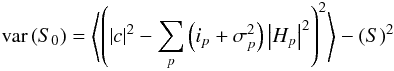 Photon noise
terms:
Photon noise
terms: ![Mathematical equation: \begin{eqnarray} &=&2\left|C\right|^{2}\sum_{p}\Lambda_{p}\left|H_{p}\right|^{2}+ CC\sum_{p}\Lambda_{p} H_{p}^{*}H_{p}^{*} + C^{*}C^{*}\sum_{p}\Lambda_{p} H_{p}H_{p}\nonumber\\ &+& \left[\sum_{p}\Lambda_{p}\left|H_{p}\right|^{2}\right]^{2} + \sum_{p}\Lambda_{p} H_{p}H_{p}\sum_{p}\Lambda_{p} H_{p}^{*}H_{p}^{*}\notag \end{eqnarray}](/articles/aa/full_html/2012/05/aa17335-11/aa17335-11-eq96.png) Read noise
terms:
Read noise
terms: ![Mathematical equation: \begin{eqnarray} + \sum_{p}\sigma_{p}^{2}\left|H_{p}\right|^{4}+ \left[ \sum_{p}\sigma_{p}^{2} \left|H_{p}\right|^{2} \right]^{2}+ \sum_{p}\sigma_{p}^{2}H_{p}H_{p}\sum_{p}\sigma_{p}^{2}H_{p}^{*}H_{p}^{*} \notag \end{eqnarray}](/articles/aa/full_html/2012/05/aa17335-11/aa17335-11-eq97.png) Coupled
terms:
Coupled
terms: 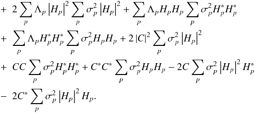
For comparison with previous work we rewrite Eq. (28) assuming DFT conditions, that read noise is constant across all pixels
( ), and that atmospheric phase fluctuations
are random and as such the cross-product of independent complex quantities average to zero:
), and that atmospheric phase fluctuations
are random and as such the cross-product of independent complex quantities average to zero:
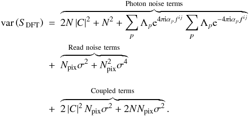 (28)Separate analysis of the photon and detector
noise terms, as is often done (see e.g. Perrin & Ridgway
2005; Le Bouquin 2005), means that the
Gaussian-Poisson coupled terms are missed. Inspection of Eq. (28) and Fig. 1 show the importance
of including these coupled terms for a wide range of photon fluxes, and therefore of
incorporating both the photon noise and read noise into a single noise model. In the above
example, for ~300 source photons on the detector, the variance on the powerspectrum is
underestimated by a factor of over 6 if cross-terms are excluded from the variance
calculation.
(28)Separate analysis of the photon and detector
noise terms, as is often done (see e.g. Perrin & Ridgway
2005; Le Bouquin 2005), means that the
Gaussian-Poisson coupled terms are missed. Inspection of Eq. (28) and Fig. 1 show the importance
of including these coupled terms for a wide range of photon fluxes, and therefore of
incorporating both the photon noise and read noise into a single noise model. In the above
example, for ~300 source photons on the detector, the variance on the powerspectrum is
underestimated by a factor of over 6 if cross-terms are excluded from the variance
calculation.
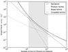 |
Fig. 1 The relative importance of the photon, read (σp = 3e−) and coupled noise terms under DFT conditions for the power spectrum variance with respect to the number of source photons detected. The area highlighted in grey is the region where the coupled terms dominate the power spectrum variance. |
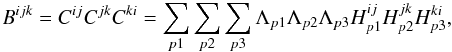
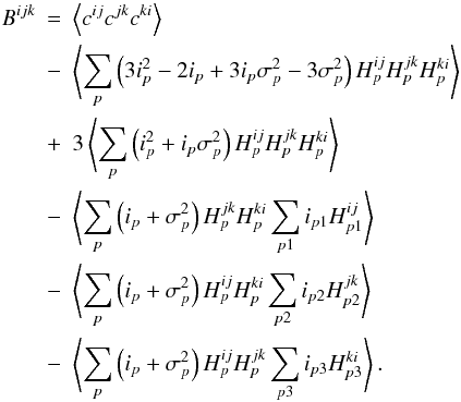
6. Bias-free bispectrum estimator
The bias-free bispectrum estimator is calculated in the same manner as the bias-free power
spectrum estimator. The definition of the bispectrum presented in Eq. (8) expands to: 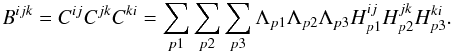 (29)Splitting the sum in Eq. (29) gives 5 terms rather than 2 as for the power
spectrum estimator. As such the derivation is quite lengthy and is given in Appendix A. We present here the bias-free bispectrum estimator,
(29)Splitting the sum in Eq. (29) gives 5 terms rather than 2 as for the power
spectrum estimator. As such the derivation is quite lengthy and is given in Appendix A. We present here the bias-free bispectrum estimator,
 :
:  (30)This equation has been verified though
computational simulations to the 0.1% level. In Sects. 7 and 8 we present the results of these
simulations regarding the closure phase, derived from the bias-free bispectrum estimator in
Eq. (30).
(30)This equation has been verified though
computational simulations to the 0.1% level. In Sects. 7 and 8 we present the results of these
simulations regarding the closure phase, derived from the bias-free bispectrum estimator in
Eq. (30).
If we assume DFT conditions so that  and an all-in-one interference pattern such
that
fij + fjk + fki = 0,
then we have
and an all-in-one interference pattern such
that
fij + fjk + fki = 0,
then we have  where we note
 and
and  .
.
If we also assume the read noise
σp = σ is constant across
all pixels rather than varying on a pixel by pixel basis then:  (31)The fact that the third order moment of the
Gaussian distribution is zero would suggest that there should be no read noise terms under
DFT conditions for constant σ, however it must be remembered that there are
second order moments in the bias correction terms which will contribute to the bias under
these conditions.
(31)The fact that the third order moment of the
Gaussian distribution is zero would suggest that there should be no read noise terms under
DFT conditions for constant σ, however it must be remembered that there are
second order moments in the bias correction terms which will contribute to the bias under
these conditions.
If we further assume that read noise is negligible
(σp = 0), then
reduces to the estimator presented by Wirnitzer (1985) accounting for the bias introduced by
photon noise alone: 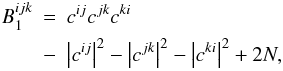 (32)where
N = ∑ pip
is the mean number of photons in the interferogram.
(32)where
N = ∑ pip
is the mean number of photons in the interferogram.
For high light levels (negligible photon noise and read noise), the
cijcjkcki
term dominates (as this goes as N3), and we reduce our estimator
further to the uncorrected estimator (correct only under zero noise conditions):
 (33)The bispectrum variance is not presented in
this paper as the
|cijcjkcki|2
term leads to a long and tedious derivation. The zealous reader is invited to calculate the
expression for the bispectrum variance if required using the method presented for
calculating the bispectrum in Appendix A.
(33)The bispectrum variance is not presented in
this paper as the
|cijcjkcki|2
term leads to a long and tedious derivation. The zealous reader is invited to calculate the
expression for the bispectrum variance if required using the method presented for
calculating the bispectrum in Appendix A.
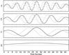 |
Fig. 2 The transform matrix, W under non-DFT conditions. The DC term shows the beam profile adopted, and the cosine (solid lines) and sine (dotted lines) components of the fringe pattern for each baseline show the deviation from integer number of fringe periods across the detector (with frequencies in the ratio 1.1 × {1:2:3}). This is similar (but with the addition of a DC term) to the visibility to pixel matrix introduced by Le Bouquin & Tatulli (2006). |
The remainder of this paper will be concerned with demonstrating the magnitude of the bias introduced when the wrong estimator is used in the presence of photon and read noise at low light levels.
7. Closure phase bias
To illustrate the magnitude of the systematic bias in a realistic observation we present the closure phase data from a set of simple simulations. We created ideal interferograms resulting from a three telescope interferometer observing a target with a known and controllable closure phase. Photon noise and read noise were added, and the bispectrum (and hence closure phase) extracted using each of the three estimators presented above. The interferograms were created under either DFT or non-DFT conditions. The fringe frequency on the detector for each baseline was set at a ratio {1:2:3} for the DFT case, and 1.1 × {1:2:3} for the non-DFT conditions. To simulate non-DFT conditions we rewrite Eq. (1) as:
![Mathematical equation: \begin{equation} i_{p} = b_{p}C^{00} + b_{p}\sum_{i < j}^{N_{\rm tel}} \mathrm{Re}\left[ C^{ij}{\rm e}^{{\rm i}2\pi \alpha_{p} f^{ij}}\right]+{\rm noise},\label{eq:simple_more_complex} \end{equation}](/articles/aa/full_html/2012/05/aa17335-11/aa17335-11-eq124.png) (34)where the beam profile,
bp is either flat:
bp = 1/Npix for
DFT conditions (as in Eq. (1)), or a cropped
Gaussian of the form:
(34)where the beam profile,
bp is either flat:
bp = 1/Npix for
DFT conditions (as in Eq. (1)), or a cropped
Gaussian of the form: ![Mathematical equation: \begin{equation} b_{p}=\frac{\exp\left[-\frac{\left(p-\mu\right)^{2}}{2\varsigma^{2}}\right]} {\sum_{p'}^{N_{\rm pix}}\exp\left[-\frac{\left(p'-\mu\right)^{2}}{2\varsigma^{2}}\right]}, \end{equation}](/articles/aa/full_html/2012/05/aa17335-11/aa17335-11-eq127.png) (35)where ς = 22 pixels and
μ is centred on the 64 pixel detector. From Eq. (34) we can construct a V2PM,
W, which is correct under DFT and non-DFT conditions. The
form of W is shown in Fig. 2 for the non-DFT conditions described. We use the Singular Value Decomposition
method to find the optimum (in terms of least squares) pseudo-inverse of
W, which gives us H. An
instrumental visibility loss was introduced such that the maximum visibility on a baseline
is |Vi| = 1/3. The results presented in
Fig. 3 are calculated using the ideal interferograms
and therefore show only the closure phase bias and suffer no variance contribution. These
are given by:
(35)where ς = 22 pixels and
μ is centred on the 64 pixel detector. From Eq. (34) we can construct a V2PM,
W, which is correct under DFT and non-DFT conditions. The
form of W is shown in Fig. 2 for the non-DFT conditions described. We use the Singular Value Decomposition
method to find the optimum (in terms of least squares) pseudo-inverse of
W, which gives us H. An
instrumental visibility loss was introduced such that the maximum visibility on a baseline
is |Vi| = 1/3. The results presented in
Fig. 3 are calculated using the ideal interferograms
and therefore show only the closure phase bias and suffer no variance contribution. These
are given by: 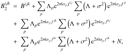 (36)and:
  (37)whilst the bias free estimator is simply:
 (38)We note the order of the indices in the DFT
terms in Eqs. (36) and (37) and that the ideal source bispectrum and
power spectrum are independent of the measurement system (weather or not if meets the DFT
conditions), whereas the bias terms implicitly assume DFT conditions for the
(38)We note the order of the indices in the DFT
terms in Eqs. (36) and (37) and that the ideal source bispectrum and
power spectrum are independent of the measurement system (weather or not if meets the DFT
conditions), whereas the bias terms implicitly assume DFT conditions for the
 and
and  estimators. Figure 3 shows a simulation of the bias present on the closure phase for the
three estimators for simulations of 120 and 300 photons per interferogram reaching the
detector.
estimators. Figure 3 shows a simulation of the bias present on the closure phase for the
three estimators for simulations of 120 and 300 photons per interferogram reaching the
detector.
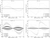 |
Fig. 3 The bias in closure phase for |
7.1. Zero read noise
In the situation where photon noise dominates the noise model
(σp = 0e−) and the instrument
is setup such that the interferograms are formed under DFT conditions,
and
both return the correct closure phase,
however is affected by a bias term resulting from
photon noise. At these light levels, the bias in becomes significant for the majority of
source closure phases.
7.2. Non-zero read noise
At low light levels the read noise on the detector becomes important and comparable to
the photon noise. Figure 3b shows simulations under
DFT conditions, as in Fig. 3a, but with
σp = 3e− read noise included.
This level of read noise is quite low compared to many of the optical detectors in use
today. We see that failing to account for read noise introduces a significant bias in
closure phase estimates for both and
. It is clear that the magnitude of the
bias term is strongly dependent on the source brightness, and that
is preferable to
under certain combinations of noise and
photon flux.
7.3. Non-DFT conditions
Deviation from DFT conditions changes the way statistical bias affects the bispectrum.
Inspection of Eq. (30) shows that the
statistical bias can affect both the real and imaginary parts of the bispectrum when
H is not the DFT. If the measurement system conforms to
DFT conditions, and the read noise is negligible or constant across all pixels, the bias
only affects the real part of the bispectrum estimators as shown when applying Eq. (31) to (30). It is also apparent that the magnitude of the bias is no longer
dependent only on the value of the closure phase, but on the value of the individual phase
of each baseline. The non-uniform beam profile causes an overlap of the fringe components
in frequency space, and the non-integral fringe frequency on the detector invalidates the
assumption that and
which led to the formulation of
. Figure 3c is provided as an example of the impact of non-DFT conditions on the closure
phase bias for a photon noise dominated instrument
(σp = 0). Note that the non-DFT
conditions change the bias terms, meaning is now biased when it was not under DFT
conditions. Figure 3d shows the effect of non-DFT
conditions on a system with photon and read noise and again there is an alteration of the
bias terms which corrects but the other estimators do not.
The grey regions on the non-DFT plots show the range of biases associated with each
estimator depending on the individual phases of the triplet producing a given closure
phase. The lines within the shaded regions represent the expectation of the closure phase
bias over all possible individual phases.
We see that the bias on the closure phase does not cancel when accumulating frames; specifically, that there is no advantage to observing in phase-unstable conditions over phase-stable conditions as a means of reducing bias. Therefore, bias-wise, one should always favor fringe-tracker assisted observations whereby the longer discrete integration times result in higher SNR, even in the photon-rich regime where fringe tracking is not strictly necessary.
7.4. Closure phase bias and statistical uncertainty
The bias is only significant at low light levels, and tends to zero as the light level increases. At low light levels the variance is also high, and we must determine the relative importance of these two processes. We present Fig. 4 which shows the relative importance of bias, Φbias, and closure phase standard deviation, ςΦ, using different estimators.
We show the number of frames, Nf, such that:
 (39)which is the number of interferograms
required to reduce the magnitude of the statistical uncertainty to that of the bias. The
closure phase standard deviation per frame, ςΦ, is given by:
(39)which is the number of interferograms
required to reduce the magnitude of the statistical uncertainty to that of the bias. The
closure phase standard deviation per frame, ςΦ, is given by:
![Mathematical equation: \begin{equation} \label{eq:cp_std_dev} \varsigma_{\Phi} = \frac{1}{\left|B^{ijk}\right|}\times\sqrt{\mathrm{var}\left[\mathrm{Im}\left(B^{ijk}_{f}\times\frac{B^{ijk*}}{\left|B^{ijk}\right|}\right)\right]}, \end{equation}](/articles/aa/full_html/2012/05/aa17335-11/aa17335-11-eq140.png) (40)where
(40)where  is the bispectrum calculated per frame
using the chosen estimator and
is the bispectrum calculated per frame
using the chosen estimator and  gives the projection of
on a unit vector perpendicular to
Bijk, and. This method is used because it
is insensitive to wrapping errors in the complex plane when the variance is large. In this
example, the magnitude of the bias and variance are measured when the source closure phase
is at 90°. The values presented in Fig. 4 were
derived using numerical simulations to the 0.1% level, and the bias contribution was
verified analytically using Eqs. (36) and
(37).
gives the projection of
on a unit vector perpendicular to
Bijk, and. This method is used because it
is insensitive to wrapping errors in the complex plane when the variance is large. In this
example, the magnitude of the bias and variance are measured when the source closure phase
is at 90°. The values presented in Fig. 4 were
derived using numerical simulations to the 0.1% level, and the bias contribution was
verified analytically using Eqs. (36) and
(37).
It can be seen in Fig. 4 that the bias is important for realistic numbers of frames (e.g. 103 frames or 25 s integration for 25 ms exposures) compared to the uncertainty for a wide range of typical light levels.
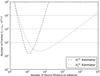 |
Fig. 4 The number of integrated frames required to reduce the statistical uncertainty to
the level of the bias for the |
8. Simulation: detection of faint companions
Simulation parameters.
Closure phase nulling is an observational techniques that allows the detection of faint companions (Chelli et al. 2009). The technique has been demonstrated by Duvert et al. (2010), detecting a 5 mag fainter companion using AMBER/VLTI around HD 59717.
Closure phase nulling uses the fact that the closure phase jumps from 0 to 180 degrees as the visibility function of the primary in the system passes through a null. The presence of a companion becomes evident as a deviation from an instantaneous phase jump. The profile of the phase jump gives information about the projected separation and flux ratio of the system components. We show that statistical bias in the closure phase leads directly to incorrect estimation of the system properties.
We follow Chelli et al. (2009) and simulate a binary system where the primary is described by a uniform disc of radius, R⋆, with a point source companion at a separation, s, with flux ratio, r. For simplicity we simulate a three telescope interferometer such that the position angle of the binary system is parallel to the frequency axis of the interferometer. The interferometer samples three frequencies {u12,u23,u13} such that u13 = u12 + u23. The instrumental parameters are given in Table 1 and we assume the instrument is functioning under DFT conditions.
The complex visibility,
Cij(u), at a given frequency,
u, is described by:  (41)which is the visibility function,
V⋆(u), of the primary:
(41)which is the visibility function,
V⋆(u), of the primary:
 (42)plus the contribution of the secondary with a
phase modulation related to the projected separation, s, and flux ratio,
r. J1 is the first order Bessel function and
R⋆ is the radius of the primary.
(42)plus the contribution of the secondary with a
phase modulation related to the projected separation, s, and flux ratio,
r. J1 is the first order Bessel function and
R⋆ is the radius of the primary.
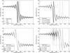 |
Fig. 5 Demonstration of the effect of bias on a closure phase measurement. Plot
a): the closure phase trace resulting from a binary pair consisting of
a resolved primary of radius R⋆ and an
unresolved secondary with flux ratio r = 0.01 for separations
(s = 10 R⋆,100 R⋆,1000 R⋆).
Plot b): the closure phase trace for the
100 R⋆ system recovered by the
three estimators. |
The ideal bispectrum is extracted from Eq. (41) using Eq. (8) and the closure phase is taken as the argument of the averaged bispectrum. The closure phase signal around the first null in the visibility profile is shown in Fig. 2 of Chelli et al. (2009) and reproduced using our simulation model in Fig. 5a in this paper for a number of companion separations (s = 10R⋆,100 R⋆,1000 R⋆). The closure phase is wrapped modulo 2π and the frequencies {u12,u23,u13} are set to the ratio {1:2:3} on the detector and scaled by the radius of the primary, R⋆. For simplicity, the baseline to fringe-frequency mapping is chosen such that it preserves the ratios of the two. The specifics of the mapping is not expected to have a significant impact on the bias. The closure phase of the primary alone (single source) is shown for comparison.
We present in Fig. 5b a simulation of the closure
phase from a 100 R⋆ separation binary with
flux ratio 0.01. returns the correct closure phase signal in
agreement with the ideal case presented by Chelli et al.
(2009). and are strongly affected by bias terms, meaning
the closure phase is significantly different. Depending which regions of the closure phase
trace are sampled by the interferometer, and would return an incorrect value for the
primary radius and companion flux ratio. Figures 5c and
d show the closure phase calculated using and respectively and the statistical uncertainty
on the measurement after 103, 104 and 105 frames calculated
using Eq. (40). We see that even for very
short total integration times (103 frames is under a minute using typical
discrete integration times) the bias still produces a significant contribution.
9. Conclusions
Interferometry offers exceptional angular resolution at the expense of sensitivity, as the collecting area is, by necessity, smaller than that of a single dish with the same resolution. In ground-based optical interferometry these sensitivity limitations are accentuated by the need for short observations to reduce the phase perturbations introduced by the atmosphere. The result is that noise levels on individual observation frames are often high, exacerbated by the need for fast read-out of the detector. Without understanding the statistical properties of the noise, bias terms are introduced when extracting information from the interferogram using the non-linear power spectrum and bispectrum constructs. We have shown in this paper that:
-
1.
Neglecting the cross terms that arise in the presence of both readnoise and photon noise leads to bias on the extraction ofinterferometric observables resulting from the statistics of thenoise.
-
2.
The statistical bias on the observables results in incorrect phisical parameters being extracted from observation data, for example the flux ratio of binary pairs or the diameter of a target as shown for the case of closure phase nulling.
To remedy this we have presented bias-free estimators for both the power spectrum and bispectrum (and hence the closure phase) which can be used in the presence of any combination of photon and read noise under any fringe encoding scheme in which the measurement equation is linear. Our bias-free estimators are presented in a format allowing easy implementation into current data reduction pipelines.
Acknowledgments
We thank the anonymous referee for constructive comments and insiteful suggestions that have undoubtedly improved this paper.
References
- Ayers, G. R., Northcott, M. J., & Dainty, J. C. 1988, J. Opt. Soc. Am. A, 5, 963 [NASA ADS] [CrossRef] [Google Scholar]
- Beletic, J. W. 1989, Opt. Comm., 71, 337 [NASA ADS] [CrossRef] [Google Scholar]
- Chelli, A., Duvert, G., Malbet, F., & Kern, P. 2009, A&A, 498, 321 [NASA ADS] [CrossRef] [EDP Sciences] [Google Scholar]
- Dainty, J. C., & Greenaway, A. H. 1979, J. Opt. Soc. Am., 69, 786 [NASA ADS] [CrossRef] [Google Scholar]
- Duvert, G., Chelli, A., Malbet, F., & Kern, P. 2010, A&A, 509, A7 [Google Scholar]
- Goodman, J. W., & Belsher, J. F. 1976a, Stanford Univ. CA Information Systems Lab [Google Scholar]
- Goodman, J. W., & Belsher, J. F. 1976b, Stanford Univ. CA Information Systems Lab [Google Scholar]
- Gordon, J., Buscher, D., & Thorsteinsson, H. 2010, in Optical and Infrared Interferometry II, ed. W. C. Danchi, F. Delplancke, & J. K. Rajagopal, Proc. SPIE, 7734, 77344A–7 [Google Scholar]
- Le Bouquin, J.-B. 2005, Imagerie par synthèse d’ouverture optique, application aux étoiles chimiquement particulières, PhD Thesis, Univ. Grenoble I [Google Scholar]
- Le Bouquin, J.-B., & Tatulli, E. 2006, MNRAS, 372, 639 [NASA ADS] [CrossRef] [Google Scholar]
- Perrin, G. 2003, A&A, 398, 385 [NASA ADS] [CrossRef] [EDP Sciences] [Google Scholar]
- Perrin, G., & Ridgway, S. T. 2005, ApJ, 626, 1138 [NASA ADS] [CrossRef] [Google Scholar]
- Roddier, F. 1987, J. Opt. Soc. Am. A, 4, 1396 [NASA ADS] [CrossRef] [Google Scholar]
- Sibille, F., Chelli, A., & Lena, P. 1979, A&A, 79, 315 [NASA ADS] [Google Scholar]
- Tatulli, E., & Duvert, G. 2007, New Astron. Rev., 51, 682 [NASA ADS] [CrossRef] [Google Scholar]
- Tatulli, E., & Le Bouquin, J.-B. 2006, MNRAS, 368, 1159 [NASA ADS] [CrossRef] [Google Scholar]
- Thorsteinsson, H., & Buscher, D. F. 2004, in New Frontiers in Stellar Interferometry, Proc. SPIE, 5491, 1498 [NASA ADS] [CrossRef] [Google Scholar]
- Wirnitzer, B. 1985, J. Opt. Soc. Am. A, 2, 14 [NASA ADS] [CrossRef] [Google Scholar]
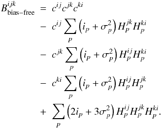
Appendix A: Derivation of the bias-free bispectrum estimator
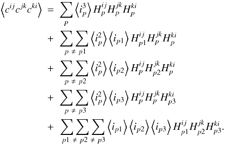
The ideal, noise-free bispectrum is given by:
 (A.1)which can be split into:
  (A.2)The equivalent expression for real data
embedded with noise when average over frames is:
(A.2)The equivalent expression for real data
embedded with noise when average over frames is:
 (A.3)which splits into:
 (A.4)Substitution of the noise model in
Eqs. (13) to (15) gives the noisy bispectrum in terms of the
ideal interferogram and associated noise:
(A.4)Substitution of the noise model in
Eqs. (13) to (15) gives the noisy bispectrum in terms of the
ideal interferogram and associated noise:
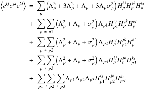 (A.5)Substituting the ideal bispectrum split sum
from Eq. (A.2) gives:
(A.5)Substituting the ideal bispectrum split sum
from Eq. (A.2) gives:
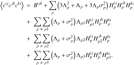 (A.6)By rearranging and substituting in for the
ensemble average over the real interferogram we find the ideal bispectrum in terms of the
noisy interferogram:
(A.6)By rearranging and substituting in for the
ensemble average over the real interferogram we find the ideal bispectrum in terms of the
noisy interferogram: 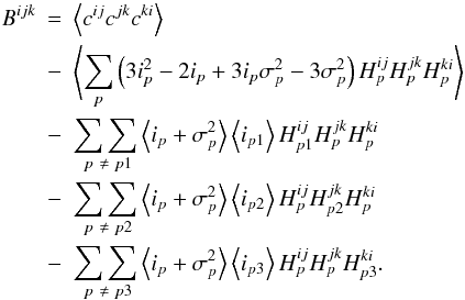 (A.7)Expanding out the double summations using the
fact that
∑ ∑ a ≠ b = ∑ ∑ a b − ∑ a = b
gives:
(A.7)Expanding out the double summations using the
fact that
∑ ∑ a ≠ b = ∑ ∑ a b − ∑ a = b
gives:
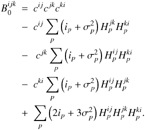
 (A.8)Cancelling terms and noting that,
 , we find the bias free bispectrum
estimator:
, we find the bias free bispectrum
estimator:
 (A.9)
(A.9)
All Tables
All Figures
|
Fig. 1 The relative importance of the photon, read (σp = 3e−) and coupled noise terms under DFT conditions for the power spectrum variance with respect to the number of source photons detected. The area highlighted in grey is the region where the coupled terms dominate the power spectrum variance. |
| In the text | |
|
Fig. 2 The transform matrix, W under non-DFT conditions. The DC term shows the beam profile adopted, and the cosine (solid lines) and sine (dotted lines) components of the fringe pattern for each baseline show the deviation from integer number of fringe periods across the detector (with frequencies in the ratio 1.1 × {1:2:3}). This is similar (but with the addition of a DC term) to the visibility to pixel matrix introduced by Le Bouquin & Tatulli (2006). |
| In the text | |
|
Fig. 3 The bias in closure phase for |
| In the text | |
|
Fig. 4 The number of integrated frames required to reduce the statistical uncertainty to
the level of the bias for the |
| In the text | |
|
Fig. 5 Demonstration of the effect of bias on a closure phase measurement. Plot
a): the closure phase trace resulting from a binary pair consisting of
a resolved primary of radius R⋆ and an
unresolved secondary with flux ratio r = 0.01 for separations
(s = 10 R⋆,100 R⋆,1000 R⋆).
Plot b): the closure phase trace for the
100 R⋆ system recovered by the
three estimators. |
| In the text | |
Current usage metrics show cumulative count of Article Views (full-text article views including HTML views, PDF and ePub downloads, according to the available data) and Abstracts Views on Vision4Press platform.
Data correspond to usage on the plateform after 2015. The current usage metrics is available 48-96 hours after online publication and is updated daily on week days.
Initial download of the metrics may take a while.