| Issue |
A&A
Volume 540, April 2012
|
|
|---|---|---|
| Article Number | L3 | |
| Number of page(s) | 5 | |
| Section | Letters | |
| DOI | https://doi.org/10.1051/0004-6361/201218897 | |
| Published online | 27 March 2012 | |
Polarization of thermal molecular lines in the envelope of IK Tauri⋆
1 Department of Earth and Space Sciences, Chalmers University of Technology, Onsala Space Observatory, 439 92 Onsala, Sweden
e-mail: This email address is being protected from spambots. You need JavaScript enabled to view it.
2 Argelander Institute für Astronomie, Universität Bonn, Auf dem Hügel 71, 53121 Bonn, Germany
3 Submillimeter Array, Academia Sinica Institute of Astronomy and Astrophysics, 645 N. Aohoku Place, Hilo, HI 96720, USA
4 European Southern Observatory, Karl Schwarzschild Str. 2, 85748 Garching bei München, Germany
Received: 27 January 2012
Accepted: 12 March 2012
Abstract
Molecular line polarization is a unique source of information about the magnetic fields and anisotropies in the circumstellar envelopes of evolved stars. Here we present the first detection of thermal CO(J = 2 → 1) and SiO(J = 5 → 4, ν = 0) polarization, in the envelope of the asymptotic giant branch star IK Tau. The observed polarization direction does not match predictions for circumstellar envelope polarization induced only by an anisotropic radiation field. Assuming that the polarization is purely due to the Goldreich-Kylafis effect, the linear polarization direction is defined by the magnetic field as even the small Zeeman splitting of CO and SiO dominates the molecular collisional and spontaneous emission rates. The polarization was mapped using the Submillimeter Array (SMA) and is predominantly north-south. There is close agreement between the CO and SiO observations, even though the CO polarization arises in the circumstellar envelope at ~800 AU and the SiO polarization at ≲ 250 AU. If the polarization indeed traces the magnetic field, we can thus conclude that it maintains a large-scale structure throughout the circumstellar envelope. We propose that the magnetic field, oriented either east-west or north-south is responsible for the east-west elongation of the CO distribution and asymmetries in the dust envelope. In the future, the Atacama Large Millimeter/submillimeter Array will be able to map the magnetic field using CO polarization for a large number of evolved stars.
Key words: stars: AGB and post-AGB / magnetic fields / polarization / submillimeter: stars
Figure 3 is available in electronic form at http://www.aanda.org
© ESO, 2012
1. Introduction
Molecular line polarization observations can provide invaluable insights into the magnetic field and/or anisotropies of the circumstellar environment of asymptotic giant branch (AGB) stars. If even a relatively weak magnetic field is present, the molecular gas in the envelope of the AGB star will show linear polarization when the magnetic sublevels of the rotational states are exposed to anisotropic emission (the Goldreich-Kylafis effect, Goldreich & Kylafis 1981, 1982). Alternatively, Morris et al. (1985) predict polarized line emission arising from molecules in an envelope that have a preferred rotation axis because of radial infrared emission from the central star. In this case, deviations from radial symmetry in the polarization angles could be due to a non-spherically symmetric envelope and/or to a (non-radial) magnetic field. While polarization observations of molecular lines, in particular of CO, in star-forming regions are relatively common (e.g. Cortes et al. 2005; Beuther et al. 2010), the only previously published significant detection of molecular line polarization around an AGB star is that of the CS(J = 2 → 1) transition around IRC+10216 (Glenn et al. 1997).
Most information about the magnetic fields in the envelopes of AGB stars is currently derived from maser observations (e.g. Vlemmings et al. 2005; Herpin et al. 2006). The maser observations reveal strong magnetic fields throughout the entire envelope (e.g. Vlemmings et al. 2011). As maser observations typically probe only a limited number of lines-of-sight through the stellar envelope, the polarization of thermal molecular lines can more easily reveal the circumstellar magnetic field morphology. A strong magnetic field is, in addition to both the binary and disk interactions, one of the possible mechanisms for shaping the typically spherical AGB winds into an aspherical planetary nebula (e.g. Balick & Frank 2002; Frank et al. 2007).
Here we present Submillimeter Array (SMA) polarization observations of the molecular lines in the circumstellar envelope of IK Tau, which is a well-studied M-type AGB star. It has a period of 500 days (Kukarkin et al. 1971), and a fairly high mass-loss rate of 1 × 10⁻⁵ M⊙ yr-1 (Ramstedt et al. 2008). The star has a rich circumstellar chemistry, as indicated by the detection of a large number (>20) of different molecular species (see e.g., Kim et al. 2010; Decin et al. 2010, for the latest results). The circumstellar gas distribution has been mapped in CO(J = 1 → 0), CO(J = 2 → 1) (Castro-Carrizo et al. 2010), and CO(J = 3 → 2) (Kim et al. 2010) emission. Castro-Carrizo et al. (2010) found a western elongation in its innermost region (of ~1000 AU), and on larger scales a flattened circumstellar envelope that is elongated in the east-west plane over ~10 000 AU. Elongated, elliptical circumstellar structures are also found on scales from a few to a few tens of AU in maps of the SiO (e.g., Cotton et al. 2010) and H2O (Bains et al. 2003) maser emission. The SiO maser observations indicate that there is a magnetic field close to the central star of 1.9–6.0 Gauss (Herpin et al. 2006).
Properties of observed lines.
2. Observations and data reduction
The observations of IK Tau were done with the SMA on October 8 2010 in the compact configuration with the lower- and upper-side band (LSB and USB) covering the frequency ranges of 216.8–220.7 GHz and 228.9–232.8 GHz, respectively. This frequency setting was specifically selected to cover the CO(J = 2 → 1) transition at 230.538 GHz, but also covered transitions of SiO, SiS, and SO. We list the detected molecular transitions in Table 1. The correlator setup provides a spectral resolution of ~0.8 MHz, which corresponds to ~1.0 km s-1 at 230 GHz. At 230 GHz, the beam size is ~3.0 × 2.6 arcsec with a position angle of 81.4°. The observations lasted for a total track of nine hours and included observations of the phase calibrator J0423-013, bandpass and polarization calibrator 3C 454.3, and the primary flux calibrators Callisto and Neptune. Based on the flux measured for J0423-013 (~2.2 Jy beam-1), we estimate that the total flux uncertainty is ≲ 10%. The right ascension (α) and declination (δ) of the phase center for the observations of IK Tau were taken to be  and
and  . The data were calibrated initially in the MIRIAD software package using the specific polarization calibration technique (Marrone & Rao 2008). Using a standard SMA polarization observing schedule, the polarization calibrator 3C 454.3 was observed regularly, covering >120° in parallactic angle. The gain calibrator J0423-013 is linearly polarized, but does not show any circular polarization. The derived amplitude gain corrections thus do not affect the amplitude calibration of the right- and left-circular polarizations produced by the SMA observation. The antenna leakage solutions were found to be up to 2% in the USB, near the CO(J = 2 → 1) line and up to 5% in the LSB, near the SiO(J = 5 → 4, ν = 0) line. The linear polarization, Pl, and electric vector polarization angle (EVPA) determined on 3C 454.3 (LSB: Pl = 0.71 ± 0.12%, EVPA = −47 ± 6°; USB: Pl = 0.80 ± 0.09, EVPA = −52 ± 2°) indicate that after calibration the remaining leakage is <0.5%. After calibration of the flux, phases, bandpass and polarization, we exported the data into the Common Astronomy Software Applications (CASA) package and performed self-calibration on the strongest spectral channel of the SiO line in the LSB. Although the SiO emission is only marginally resolved, we used the initial total intensity image as a model. This assumes that the SiO emission has no significant circular polarization, which was verified to be the case. The SiO self-calibration solutions were compared with self-calibration solutions derived from the strongest spectral channel of the CO line (also following an initial image as a starting model) in the USB and were found to be identical. We then applied the SiO self-calibration solutions to both LSB and USB as the SiO solutions were obtained using data with higher signal-to-noise ratios. Maps of the total intensity Stokes I and the linear polarization intensities Stokes Q and U were created using “briggs” weighting. To optimize the polarization detection, spectral channels were averaged over an interval of 5 km s-1 for the CO, SiS, and SO lines and 2.5 km s-1 for the SiO lines. As a results, the channel root-mean-square (rms) noise ranges from ~35 mJy beam-1 for the CO line to ~65 mJy beam-1 for the SiO line. We note that the noise in the LSB is ~30% higher than that in the USB. We also imaged the CO line without self-calibration in order to test the effect of self-calibration on the polarization. The EVPAs and linear polarization structure were found to be the same as when self-calibration was applied. Only the significance of the polarization detections decreased by ~15%.
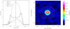 |
Fig. 1 (Left) Spectra of the observed molecular lines in the envelope of IK Tau. The emission is summed over all SMA baselines. The vertical line indicates the VLSR = 34 km s-1 stellar velocity. (right) The stellar continuum and dust emission (color) and integrated CO(2–1) line emission (contours) of IK Tau. The contours are drawn at 10,20,40,80, and 160 Jy beam-1 km s-1. |
3. Results
Emission was detected from the CO(J = 2 → 1), SiO(J = 5 → 4, ν = 0), SO(J = 6 → 5), and SiS(J = 12 → 11) transitions, hereafter indicated by CO(2–1), SiO(5–4), SO(6–5), and SiS(12–11). The spectra of these transitions is shown in Fig. 1 (left). Significant polarization was detected for the CO(2–1) and SiO(5–4) lines shown in Figs. 2 and 3. To determine the significance of the weak linear polarization signal, we carefully removed the positive bias, which was introduced when the Stokes Q and U measurements were combined to produce the linearly polarized emission ( ), following Wardle & Kronberg (1974).
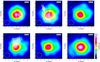 |
Fig. 2 The polarization of the CO(2–1) line at 230.538 GHz in the circumstellar envelope of IK Tau. Channels are averaged across intervals of 5 km s-1 width and are labeled according to the velocity at the lower end of the spectral bin. The color indicates the CO emission and the contours are the linearly polarized intensity. Contours are drawn at a significance of 3 and 4σ (debiased, see text). The line segments indicate the electric vector polarization angle (EVPA). The beam size is indicated in the lower left corner of each panel. |
As the errors in Pl are not Gaussian-distributed, the significance is defined by determining the probability intervals. The contours in Figs. 2 and 3 thus correspond to the 3σ = 99.73% and higher probability intervals. The peak of the linear polarization corresponds to 4.9σ and 6.8σ detections for the CO(2–1) and SiO(5–4) lines, respectively. The maximum polarization fractions are listed in Table 1. The EVPAs for both CO(2–1) and SiO(5–4) are predominantly oriented north-south. The polarization angle of CO(2–1) ranges from approximately −10° in the southern part of the envelope in the channel around VLSR = 25 km s-1 to ~10° in the northern part in the channels with VLSR = 25 and 35 km s-1. A somewhat smaller spread (−7 to 4°) is seen for the SiO(5–4) line, although for this line the polarized emission is confined close to the peak of the Stokes I emission. The measurement uncertainties for the EVPA ranges from 6–10° for CO(2–1) and 4–10° for SiO(5–4). This indicates that the difference in EVPA between the northern and southern part of the CO envelope is potentially real.
4. Discussion
4.1. Polarized molecular line emission
The models of polarized molecular line-emission prescribe that the polarization can be caused by a preferred radiation direction (Morris et al. 1985) or an interaction with a magnetic field (Goldreich & Kylafis 1981, 1982). In the first case, the stellar radiation will lead to polarization predominantly perpendicular to the radial direction. When the magnetic field is non-radial, and strong enough to determine the molecular alignment axis, competition between the field and radiation direction will change the polarization characteristics. Morris et al. (1985) state that for any field stronger than a few μG, the magnetic field in the envelope determines the molecular alignment axis. For the Goldreich-Kylafis effect, the linear polarization is oriented along the magnetic field as long as the Zeeman splitting dominates the collisional and spontaneous emission rates.
The importance of the magnetic field in determining the polarization characteristics of molecular line emission was estimated in Kylafis (1983). We used their Eqs. (1)–(3), with the parameters adjusted to describe the CO(2–1) transition, and assumed a magnetic field strength ~1 μG in the CO(2–1) region, a magnetic moment μ = −0.27μN (with μN the nuclear magneton), and a reduced dipole matrix element d = 0.11 debye. It is then clear that a hydrogen number density ≲ 3 × 106 cm-3 is sufficient for the magnetic field to determine the direction of the polarized CO(2–1) emission. As the SiO(5–4) emission originates from closer to the star, the stronger magnetic field will also result in a dominant Zeeman splitting. Owing to the field strength measured around IK Tau and other AGB stars (>1 mG within several hundred AU, Vlemmings et al. 2005), the linear polarization thus likely traces the magnetic field morphology when assuming the polarization originates from the Goldreich-Kylafis effect. As indicated in Kylafis (1983) the CO EVPAs, arising from the Goldreich-Kylafis effect, are determined by the magnetic field direction on the plane of the sky. This is shown irrespective of the direction of the velocity gradient in the envelope, except that the relative optical depth caused by the velocity gradient determines whether the EVPAs are parallel or perpendicular to the magnetic field direction.
The observed linear polarization fraction is, however, larger than predicted from the general Goldreich-Kylafis effect. Cortes et al. (2005) predict ≲ 3% for CO(2–1) when the optical depth is low (τ ~ 1). They also show that higher fractional polarization can be achieved when a strong anisotropic radiation source is present. However, in that case, the polarization direction is determined by the anisotropic radiation field that, in the case of a circumstellar envelope, would cause tangential polarization. As the linear polarization in the envelope of IK Tau is neither tangential nor purely radial as predicted by Deguchi & Watson (1984) from multi-level calculations involving infra-red excitation, it is unlikely that the anisotropic stellar radiation field contributes significantly. The high polarization fraction is potentially caused by other anistotropies in the circumstellar enviroment. More detailed modeling will be required to determine the origin of the large fractional polarization.
4.2. The magnetic field of IK Tau
For both the CO(2–1) and SiO(5–4) lines, we observe polarization that is slightly offset from the peak of the total intensity emission. For CO(2–1), the largest polarization fraction is found in the south part of the blue-shifted side of the envelope and in the north part of the red-shifted side. The observed structure in the polarized emission is likely an effect of similar structure in the optical depth, as the largest fractional polarization is found when the optical depth τ ~ 1.
As the circumstellar magnetic field strength has been shown to be sufficient to determine the molecular alignment axis, the polarization vectors are either parallel or perpendicular to the magnetic field direction in the framework outlined by Kylafis (1983). In that case, the overall field geometry is predominantly either east-west or north-south. As only relatively few independent polarization vectors are measured, a more accurate magnetic field reconstruction will require more sensitive observations. We are able to compare the EVPA direction derived from the CO(2–1) and SiO(5–4) EVPAs with the previous measurements made of the SiO maser polarization by Herpin et al. (2006). In that paper, the 86 GHz SiO maser linear polarization, averaged over several individual maser features with the 30-m IRAM telescope, was found to have an EVPA of 170–180° for the masers blue-shifted with respect to the star. The EVPA then rotates to 140–160° for the red-shifted masers. Thus, the CO(2–1) and SiO(5–4) EVPAs are, for the blue-shifted emission, remarkably consistent with the averaged 86 GHz SiO masers. However, for the 43 GHz SiO masers, Cotton et al. (2010) found, from high-angular resolution interferometric observations a much more complex and variable polarization structure. The CO(2–1) polarized emission is detected about 3″ (~800 AU) from the star and that of SiO(5–4) originates within ~1″ (~250 AU), which could be an indication that, as in the case of the supergiant VX Sgr (Vlemmings et al. 2011), the magnetic field has a large-scale component that is preserved throughout the envelope. As the field is then mainly oriented either east-west or north-south, it might be directly related to the slight east-west extent seen in the circumstellar CO envelope (Castro-Carrizo et al. 2010, and Fig. 1, right) and the east-west asymmetry in the dust distribution (Weiner et al. 2006). Magneto-hydrodynamical simulations indicate, for example, that a dipole magnetic field in a circumstellar envelope can result in equatorially enhanced density profiles (Matt et al. 2000). However, we note that the elliptical SiO maser structure is oriented more in a northeast-southwest direction (Cotton et al. 2010).
4.3. Prospects for ALMA
Observations such as the ones presented here will undergo a revolution when the Atacama Large Millimeter/submillimeter Array (ALMA) becomes fully operational. With 50 antennas and in typical weather conditions, ALMA will reach the same sensitivity in the linear polarization as reached with the SMA (assuming similar angular resolution and spectral binning) in less than two seconds. In particular for IK Tau, it will be able to improve the observations to a 10σ linear polarization detection with higher spatial resolution (1″ × 1″) and velocity resolution (2 km s-1) in less than 20 min on-source observing time. While the SMA observations filter out a large fraction of the CO(2–1) flux, ALMA with the compact array and total power antennas will recover most of the emission and reach a similar polarization detection level even for the evolved stars with weaker CO emission. Thus, on the basis of the SMA observations presented here, with ALMA it will be possible to map out the CO(2–1) and other molecular-line linear polarization in great detail for a large number of (post-)AGB stars and planetary nebulae in a relatively
short time. As a consequence, ALMA polarization observations will provide unique information on the magnetic field morphology around evolved stars.
5. Conclusions
We have presented the first observations of polarized CO(J = 2 → 1) and SiO(J = 5 → 4, ν = 0) emission in the circumstellar envelope of an evolved star. As the polarization is neither radial nor tangential, the linear polarization does not match typical predictions for linear polarization induced solely by an anisotropic radiation field or optical depth effects. It thus potentially traces the magnetic field even when influenced by anisotropic emission from the central AGB star IK Tau. In that case, the magnetic field is oriented either east-west or north-south and a good correspondence is found between the direction derived from the CO polarization at ~800 AU from the central star and that from the thermal SiO at ~250 AU. The slight east-west elongation of the CO and the previously observed dust asymmetry could be related to the large-scale magnetic-field morphology. Further observations and theoretical work are needed to properly understand the influence of the magnetic field and the envelope and radiation anisotropies on the circumstellar linear polarization. It may then be possible to fully describe the circumstellar magnetic field structure. In particular, ALMA will be able to uniquely map out polarization for a significant sample of AGB and post-AGB objects.
Online material
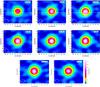 |
Fig. 3 As Fig. 2 for the SiO(5–4) ν = 0 line at 217.105 GHz. In this case, channels are averaged over intervals of 2.5 km s-1 and contours are drawn at debiased polarized intensity levels of 3,4,5, and 6σ. |
Acknowledgments
The authors thank the anonymous referee for comments that significantly improved the paper. This research was supported by the Deutsche Forschungsgemeinschaft (DFG; through the Emmy Noether Research grant VL 61/3-1).
References
- Bains, I., Cohen, R. J., Louridas, A., et al. 2003, MNRAS, 342, 8 [NASA ADS] [CrossRef] [Google Scholar]
- Balick, B., & Frank, A. 2002 , ARA&A, 40, 439 [Google Scholar]
- Beuther, H., Vlemmings, W. H. T., Rao, R., & van der Tak, F. F. S. 2010, ApJ, 724, L113 [Google Scholar]
- Castro-Carrizo, A., Quintana-Lacaci, G., Neri, R., et al. 2010, A&A, 523, A59 [NASA ADS] [CrossRef] [EDP Sciences] [Google Scholar]
- Cortes, P. C., Crutcher, R. M., & Watson, W. D. 2005, ApJ, 628, 780 [NASA ADS] [CrossRef] [Google Scholar]
- Cotton, W. D., Ragland, S., Pluzhnik, E. A., et al. 2010, ApJS, 187, 107 [NASA ADS] [CrossRef] [MathSciNet] [Google Scholar]
- Decin, L., Justtanont, K., De Beck, E., et al. 2010, A&A, 521, L4 [CrossRef] [EDP Sciences] [Google Scholar]
- Deguchi, S., & Watson, W. D. 1984, ApJ, 285, 126 [NASA ADS] [CrossRef] [Google Scholar]
- Frank, A., De Marco, O., Blackman, E., & Balick, B. 2007, unpublished [arXiv:0712.2004] [Google Scholar]
- Goldreich, P., & Kylafis, N. D. 1981, ApJ, 243, L75 [NASA ADS] [CrossRef] [Google Scholar]
- Goldreich, P., & Kylafis, N. D. 1982, ApJ, 253, 606 [NASA ADS] [CrossRef] [Google Scholar]
- Glenn, J., Walker, C. K., Bieging, J. H., & Jewell, P. R. 1997, ApJ, 487, L89 [NASA ADS] [CrossRef] [Google Scholar]
- Herpin, F., Baudry, A., Thum, C., Morris, D., & Wiesemeyer, H. 2006, A&A, 450, 667 [NASA ADS] [CrossRef] [EDP Sciences] [Google Scholar]
- Kim, H., Wyrowski, F., Menten, K. M., & Decin, L. 2010, A&A, 516, A68 [NASA ADS] [CrossRef] [EDP Sciences] [Google Scholar]
- Kukarkin, B. V., Kholopov, P. N., Pskovsky, Y. P., et al. 1971, General Catalogue of Variable Stars, 3rd edn., 0 [Google Scholar]
- Kylafis, N. D. 1983, ApJ, 267, 137 [NASA ADS] [CrossRef] [Google Scholar]
- Matt, S., Balick, B., Winglee, R., & Goodson, A. 2000, ApJ, 545, 965 [NASA ADS] [CrossRef] [Google Scholar]
- Marrone, D. P., & Rao, R. 2008, Proc. SPIE, 7020, 60 [NASA ADS] [Google Scholar]
- Morris, M., Lucas, R., & Omont, A. 1985, A&A, 142, 107 [NASA ADS] [Google Scholar]
- Ramstedt, S., Schöier, F. L., Olofsson, H., & Lundgren, A. A. 2008, A&A, 487, 645 [NASA ADS] [CrossRef] [EDP Sciences] [Google Scholar]
- Vlemmings, W. H. T., van Langevelde, H. J., & Diamond, P. J. 2005, A&A, 434, 1029 [NASA ADS] [CrossRef] [EDP Sciences] [Google Scholar]
- Vlemmings, W. H. T. 2007, IAU Symp., 242, 37 [NASA ADS] [Google Scholar]
- Vlemmings, W. H. T., Humphreys, E. M. L., & Franco-Hernández, R. 2011, ApJ, 728, 149 [NASA ADS] [CrossRef] [Google Scholar]
- Wardle, J. F. C., & Kronberg, P. P. 1974, ApJ, 194, 249 [NASA ADS] [CrossRef] [Google Scholar]
- Weiner, J., Tatebe, K., Hale, D. D. S., et al. 2006, ApJ, 636, 1067 [NASA ADS] [CrossRef] [Google Scholar]
All Tables
All Figures
|
Fig. 1 (Left) Spectra of the observed molecular lines in the envelope of IK Tau. The emission is summed over all SMA baselines. The vertical line indicates the VLSR = 34 km s-1 stellar velocity. (right) The stellar continuum and dust emission (color) and integrated CO(2–1) line emission (contours) of IK Tau. The contours are drawn at 10,20,40,80, and 160 Jy beam-1 km s-1. |
| In the text | |
|
Fig. 2 The polarization of the CO(2–1) line at 230.538 GHz in the circumstellar envelope of IK Tau. Channels are averaged across intervals of 5 km s-1 width and are labeled according to the velocity at the lower end of the spectral bin. The color indicates the CO emission and the contours are the linearly polarized intensity. Contours are drawn at a significance of 3 and 4σ (debiased, see text). The line segments indicate the electric vector polarization angle (EVPA). The beam size is indicated in the lower left corner of each panel. |
| In the text | |
|
Fig. 3 As Fig. 2 for the SiO(5–4) ν = 0 line at 217.105 GHz. In this case, channels are averaged over intervals of 2.5 km s-1 and contours are drawn at debiased polarized intensity levels of 3,4,5, and 6σ. |
| In the text | |
Current usage metrics show cumulative count of Article Views (full-text article views including HTML views, PDF and ePub downloads, according to the available data) and Abstracts Views on Vision4Press platform.
Data correspond to usage on the plateform after 2015. The current usage metrics is available 48-96 hours after online publication and is updated daily on week days.
Initial download of the metrics may take a while.