| Issue |
A&A
Volume 540, April 2012
|
|
|---|---|---|
| Article Number | A3 | |
| Number of page(s) | 12 | |
| Section | Stellar atmospheres | |
| DOI | https://doi.org/10.1051/0004-6361/201118623 | |
| Published online | 13 March 2012 | |
CNO and F abundances in the globular cluster M 22 (NGC 6656)
1 Departamento de Astronomía y AstrofísicaPontificia Universidad Católica de Chile, Av. Vicuña Mackenna 4860, Macul, 782-0436 Santiago, Chile
2 Research School of Astronomy and Astrophysics, The Australian National University, Cotter Road, Weston, ACT 2611, Australia
e-mail: This email address is being protected from spambots. You need JavaScript enabled to view it.
3 Departamento de Astronomia, IAG, Universidade de São Paulo, Rua do Matão 1226, Cidade Universitária, 05508-900 São Paulo, Brazil
Received: 12 December 2011
Accepted: 3 February 2012
Abstract
Context. Recent studies have confirmed the long standing suspicion that M 22 shares a metallicity spread and complex chemical enrichment history similar to that observed in ω Cen. M 22 is among the most massive Galactic globular clusters and its color–magnitude diagram and chemical abundances reveal the existence of sub-populations.
Aims. To further constrain the chemical diversity of M 22, necessary to interpret its nucleosynthetic history, we seek to measure relative abundance ratios of key elements (carbon, nitrogen, oxygen, and fluorine) best studied, or only available, using high-resolution spectra at infrared wavelengths.
Methods. High-resolution (R = 50 000) and high S/N infrared spectra were acquired of nine red giant stars with Phoenix at the Gemini-South telescope. Chemical abundances were calculated through a standard 1D local thermodynamic equilibrium analysis using Kurucz model atmospheres.
Results. We derive [Fe/H] = −1.87 to −1.44, confirming at infrared wavelengths that M 22 does present a [Fe/H] spread. We also find large C and N abundance spreads, which confirm previous results in the literature but based on a smaller sample. Our results show a spread in A(C+N+O) of ~ 0.7 dex. Similar to mono-metallic globular clusters, M 22 presents a strong [Na/Fe]-[O/Fe] anticorrelation as derived from Na and CO lines in the K band. For the first time we recover F abundances in M 22 and find that it exhibits a 0.6 dex variation. We find tentative evidence for a flatter A(F)-A(O) relation compared to higher metallicity globular clusters.
Conclusions. Our study confirms and expands upon the chemical diversity seen in this complex stellar system. All elements studied to date show large abundance spreads which require contributions from both massive and low mass stars.
Key words: Galaxy: abundances / globular clusters: individual: M 22 (NGC 6656) / stars: abundances
© ESO, 2012
1. Introduction
The idea that globular clusters (GCs) are the simplest example of a stellar population (Renzini & Buzzoni 1986), that is, all their stars having the same age and chemical composition, has been challenged over the years. On the one hand, detailed chemical abundance analyses have shown that almost all GCs present negligible internal abundance variations of iron-peak elements, whereas an unexpected large star-to-star abundance variation is found for light elements (Li, C, N, O, Na, Mg and Al), within which a strong anticorrelation is present in the O:Na and Mg:Al pairs. As these anomalies are found in both giant stars and turnoff and sub-giant stars (see e.g. Cannon et al. 1998), the most plausible explanation is that they are primordial in origin, that is, they must be present in the gas from which these stars were formed. In this scenario, intermediate mass (3–8 M⊙) asymptotic giant branch (AGB) and massive stars acting in the early stages of globular cluster formation are the strongest polluter candidates (see Gratton et al. 2004, for an extensive review). Additionally, very deep photometry of some of the most massive Galactic GCs has revealed color-magnitude diagrams (CMDs) that display multiple stellar populations (see e.g. Piotto 2009, and references therein) and such behavior has not yet been fully understood (see, e.g., Valcarce & Catelan 2011, for a recent review and alternative scenario).
In this context NGC 6656 (M 22, l = 9.89°, b = −7.55°), an inner halo GC located at R⊙ = 3.2 kpc, is one of the most interesting GCs for detailed abundance analysis because previous photometric (e.g. Hesser & Harris 1979) and spectroscopic (e.g. Norris & Freeman 1983) studies revealed a chemical heterogeneity for this cluster. Photometrically, Piotto (2009) identified multiple stellar populations on the sub-giant branch of M 22. Detailed abundance analyses based on a few stars and using high-resolution CCD spectra, albeit limited to a spectral resolution of R ~ 20 000 (see, e.g., Gratton 1982; Pilachowski et al. 1982; Brown et al. 1990; Brown & Wallerstein 1992, for more details) found conflicting results regarding the abundance spread in M 22. Studying six giant stars in M 22, Pilachowski et al. (1982) found a large spread of 0.5 dex in metallicity for this GC. These findings were also supported by Lehnert et al. (1991) who studied 10 giant stars and found a variation of Δ[Fe/H] = +0.3 dex. On the other hand, others found no evidence for a metallicity dispersion (e.g. Cohen 1981; Gratton 1982; Ivans et al. 2004). More recently, a coherent picture is developing which confirms a metallicity spread in M 22 using optical spectra with a range in resolution (R = 2000–60 000; Marino et al. 2009, 2011; Da Costa et al. 2009). Thus, photometric and spectroscopic studies suggest that M 22 shares striking similarities to ω Cen – the most massive Galactic globular cluster that shows a wide range of chemical abundance variations, as it was first proposed by Hesser et al. (1977).
CNO group abundances are especially important for understanding the properties of multiple population GCs (Cassisi et al. 2008). For M 22, CNO group abundances have been reported in the literature for a few stars. Using photometry, Frogel et al. (1983) reported a large spread in CO within M 22. Spectroscopically, Norris & Freeman (1983) found a chemical inhomogeneity in M 22 based on the behavior of the CH, CN and A(Ca) spectral indices for a large number of giant stars (see also Anthony-Twarog et al. 1995, for a larger sample). In particular, they found a direct correlation between the variation of CN and the Ca II H and K lines. Brown et al. (1990) studied seven stars in M 22 and found a large range of N abundances in their sample that was difficult to explain by CNO cycling and mixing. Kayser et al. (2008) compared the relative CN and CH line strengths of 97 stars and concluded that the number of CN-weak stars in M 22 is higher than that of the CN-strong. More recently Marino et al. (2011) studied 35 red giants in M 22 using high-resolution optical spectra and found C-N anticorrelations in the subsample analyzed.
Fluorine is a relatively poorly studied element that may provide key insights into globular cluster chemical evolution. Jorissen et al. (1992) were the first to determine F abundances outside the solar system. Almost two decades later, it has been known that F can be synthesized in AGB stars, and it is produced in the He-intershell along with C and s-process elements (Jorissen et al. 1992; Lugaro et al. 2004); however, the nucleosynthetic origin of fluorine in the Galaxy is still a mystery (see, e.g., the Introduction of Alves-Brito et al. 2011, for a recent summary). Despite its importance as a tracer of AGB nucleosynthesis, F has been only measured in three Galactic GCs to date – ω Cen (Cunha et al. 2003), M 4 (Smith et al. 2005) and NGC 6712 (Yong et al. 2008).
In this work we present the first abundance estimates of C, N, O, F, Na and Fe for giant stars in M 22 using spectra taken at infrared wavelengths through the high-resolution, near-infrared Phoenix spectrograph at Gemini-South. We investigate the CNO group and Fe abundance variations in M 22 and the behavior of F with respect to O and also to the s-process elements. These data provide additional critical constraints upon the role of massive and low mass stars in the chemical evolution of M 22. Finally, we compare our results with chemical abundance patterns in GCs and field stars in order to provide valuable information on how the different Galactic populations were formed and have evolved.
The paper is organized as following. Section 2 describes the observations. Section 3 presents the data analysis. The results and discussions are outlined in Sect. 4. Finally, Sect. 5 summarizes the main conclusions.
2. Observations
In this work we take advantage of the high-resolution infrared spectrograph Phoenix at Gemini-South (Hinkle et al. 2003) to carry out a detailed abundance analysis of bright giant stars in M 22. The targets were selected based on the study of proper motions and radial velocities presented by Peterson & Cudworth (1994) and, additionally, by analysing the CMD from the Two Micron All Sky Survey (2MASS, Skrutskie et al. 2006). We selected 11 bright giant stars that could be observed with reasonable exposure-times, 6.93 ≤ H2MASS ≤ 7.97 mag, with high membership probabilities (P > 87%; see Fig. 1). In addition, for a more reliable comparison with results previously presented for this cluster, we included in our sample four out of six stars studied by Pilachowski et al. (1982), who found a spread of 0.5 dex in metallicity for these four stars.
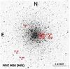 |
Fig. 1 The finding chart of M 22 from the optical Digitized Sky Survey. The targets are clearly marked following the nomenclature defined in Peterson & Cudworth (1994). The field’s orientation is shown and the displayed sky area is of 15 × 15 arcmin2. The coordinates (J2000) of the image center are |


The stars were observed in service mode between 2009 March-July. The slit width-size of 0.34 arcsec was used in order to reach a resolution of R = 50 000. To study the sample, our observing programme was executed at two different filters, H6420 and K4308, which cover a wavelength range from 1552 to 1558 nm (H band) and from 2330 to 2340 nm (K band). Each target was observed at two different positions along the slit and the exposure times ranged from 316 to 1220 s. In addition to standard calibrations (10 bias and 10 dark exposures), in each night of our observing run we included spectra of rapidly rotating hot stars in order to correct the spectra for fringing (H band) and telluric lines (K band). The nominal signal-to-noise ratio (S/N) per pixel in the H band ranges from 60–140, while in the K band it varies from 130–160. In Table 1 we list the stars, along with their magnitudes, date of observations and S/N estimates in both bands. The spectra were reduced with IRAF1 employing standard procedures as described in details in Smith et al. (2002) and Meléndez et al. (2003), which include dark and sky subtraction, flatfield correction, spectrum extraction, wavelength calibration and telluric correction.
As noted in Alves-Brito et al. (2011), the CNO group elements are better studied in the infrared, where their lines are more numerous and the continuum is formed deepest in the layers of the stellar atmosphere due to the opacity minimum of H− near the H band. For red giant stars, F measurements are only available from the HF molecule in the K band.
Program stars.
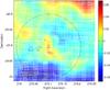 |
Fig. 2 Extinction map for M 22 in equatorial coordinates (J2000). The small and large circles indicate, respectively, the GC’s center and the area where the program stars (crosses) lie in the GC’s field. The color bar gives the excesses E(B − V) for the extinction map. The zero point is arbitrary and it is calculated by comparison with isochrones (see Alonso-Garcia et al. 2011, 2012, for more details on the techniques and methods used to create this figure). The orientation is different from Fig. 1 (North-East points to the upper right corner). |
3. Data analysis
3.1. Atmospheric parameters
3.1.1. Photometry
Due to its relatively low galactic latitude, M 22 presents a high mean interstellar extinction, E(B − V) = 0.34 (Harris 1996). In addition, as M 22 is projected relatively near the Galactic center (l = 9.89°, b = −7.55°), the extent of its differential extinction has been a controversial topic. Using the Balmer strengths of blue horizontal branch stars, Crocker (1988) found a ΔE(B − V) less than 0.08 mag for M 22. Similar values were also found by Minitti et al. (1992) using polarization. Based on wide-field B, V and I photometry, Monaco et al. (2004) found ΔE(B − V) ~ 0.06 mag. They argue that the likely multiple stellar populations in this cluster is just an artifact created by the reddening variations across the area of the GC. Alternatively, we show in Fig. 2 the extinction map for M 22 that was kindly provided by Dr. Javier Alonso-Garcia. As can be seen, the map suggests that the total range in E(B − V) is small, less than 0.06 mag within approximately 15 arcmin from the GC’s center. The differential extinction is particularly important because it adversely impacts upon the assignment of star’s membership probabilities and also increases the uncertainties on the temperatures and surface gravities obtained photometrically in reddened GCs.
To obtain the photometric effective temperatures, we used the magnitudes listed in Table 1 altogether with the empirical temperature scale of Alonso et al. (1999). The 2MASS magnitudes were transformed to the Telescopio Carlos Sánchez (TCS) system using relations by Carpenter (2001) and Alonso et al. (1998). The colors were dereddened by adopting a fixed reddening E(B − V) = 0.34 (Harris 1996) and reddening ratios E(V − K)/E(B − V) = 2.744 and E(J − K)/E(B − V) = 0.52 (Rieke & Lebofsky 1985). However, as the (V − K)0 colors provide more accurate temperatures due to its long baseline in wavelength, we have chosen to adopt the TV − K as the final photometric temperatures for our program stars. Alonso’s calibrations are metallicity dependent, and thus we have adopted a metallicity of [Fe/H]2 = −1.64 for M 22 (Harris 1996).
Stellar parameters, radial velocities, and membership probabilities.
Surface gravities (log g) were derived with the classical relation, adopting T⊙ = 5780 K, Mbol⊙ = 4.75, log g⊙ = 4.44 dex, and M∗ = 0.80 M⊙. In addition, we assumed a distance modulus of (m − M)V = 13.60, and bolometric corrections BCV as given by Alonso et al. (1999).
3.1.2. Spectroscopy
All program stars were recently studied by Marino et al. (2011) using high-resolution optical spectra (37 500 ≤ R ≤ 60 000). Hence, due to both the controversial issues regarding the derivation of the photometric atmospheric parameters and also to the fact that there are no numerous iron lines at infrared wavelengths, we adopted the spectroscopic atmospheric parameters derived by Marino et al. (2011) using numerous Fe lines. However, we have used our own infrared data to constrain the final metallicities, which were iteratively adjusted along with the CNO abundances.
Final atmospheric parameters and kinematics are presented in Table 2. Interestingly, examination of Table 2 reveals that the photometric parameters, which were obtained by assuming a uniform reddening of E(B − V) = 0.34 mag, are in good agreement with the spectroscopic ones. The mean difference (photometry – spectroscopy) is –46 ± 19 (σ = 56) K for Teff and +0.08 ± 0.06 (σ = 0.20) dex for log g. Because the spectroscopic analysis is reddening free, these results indicate that there is no significant reddening variation for the stars studied. We reiterate that Fig. 2 also suggests that there is no significant differential reddening for the program stars.
We note, however, that the comparison of the stellar spectroscopic parameters adopted in this work and previous literature values (see, e.g. Pilachowski et al. 1982; Gratton 1982; Wallerstein et al. 1987; Smith & Suntzeff 1989; Brown et al. 1990) reveals some discrepancies. These differences vary significantly, for a given star, depending on which literature study is adopted for comparison. We believe that such discrepancies are not only due to the different parameters used (e.g., reddening, distance modulus, colors) but also as a consequence of the different techniques of analysis employed by the different authors. For example, for the star III-3, Brown et al. (1990) obtained Teff = 4500 K, log g = 0.7 dex and ξ = 2.3 km s-1, while Pilachowski et al. (1982) found Teff = 4100 K, the same log g and a higher microturbulent velocity, ξ = 3.5 km s-1.
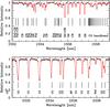 |
Fig. 3 Observed (points) and best synthetic (lines) spectra of M 22 III-52 in the H (top) and K (bottom) bands. Adopted abundances can be found in Tables 2 and 4. Several atomic and molecular lines are identified. |
3.2. Spectral synthesis
To measure the chemical compositions of C, N, O, F, Na and Fe in the H band at 1555 nm (OH, CO, CN and Fe) and in the K band at 2330 nm (CO, HF and Na) we used the same line list as used in previous studies dedicated to the analysis of giant stars in the infrared (see, e.g. Meléndez et al. 2003, 2008; Yong et al. 2008, for more details). The HF (1–0) R9 line at 2335 nm presents χ = 0.480 eV and log gf = −3.955 dex. We have assumed isotopic ratios 12C/13C = 5 for all stars.
Elemental abundances were obtained using Kurucz model atmospheres (Castelli et al. 1997) and the local thermodinamical equilibrium (LTE) spectral synthesis code MOOG (Sneden 1973). Using the spectroscopic atmospheric parameters given in Marino et al. (2011) as a first input, we reobtained the Fe abundances and using OH lines in the H band we obtained the [O/Fe] ratios for the sample. Carbon abundances were then obtained by using the CO molecular bandhead at 1558 nm. Next, nitrogen abundances were derived from CN molecular lines in the H band. The carbon abundances were also checked using the numerous CO lines in the K band. Since the CNO abundances are coupled, we iterated until self-consistent abundances were achieved. Na and F were obtained by using the NaI line at 2337 nm and the HF molecular line at 2335 nm, respectively. All observed spectra were convolved with Gaussian functions in order to take the instrumental profile into account as well other broadening effects such as macroturbulence and rotation. Except for star III-3, the synthetic spectra in the K band, convolved with a Gaussian of typical FWHM 10 km s-1, were slightly broader than those in the H band by approximately 2 km s-1. Figures 3–9 illustrate the fit of synthetic spectra to the observed ones in both H and K bands.
3.3. Error analysis
As previously stated, the exact reddening for M 22 is somewhat uncertain. To obtain the photometric atmospheric parameters we have adopted and applied a uniform reddening correction of E(B − V) = 0.34 mag for all stars. Had we changed the E(B − V) value by +0.06 dex, the temperature would increase by 150 K. Additionally, that would lead to an uncertainty of approximately 0.5 kpc in the distance, which would translate into an uncertainty in log g of approximately +0.20 dex. Since ΔE(B − V) is likely smaller than 0.06 for the cluster in general and for the program stars in particular (see Fig. 2), the errors in Teff and log g mentioned above should be smaller. A typical uncertainty of 0.03 in E(B − V) would lead to an error of about 75 K in Teff and about 0.1 dex in log g. These uncertainties are in good agreement with those estimated by Marino et al. (2011) for the spectroscopic parameters. As explained in Sect. 3.1.2, the mean difference between the photometric and spectroscopic parameters is of –46 ± 19 (σ = 56) K for Teff and +0.08 ± 0.06 (σ = 0.20) dex for log g.
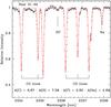 |
Fig. 4 Example of spectral synthesis in M 22 III-52 in the K band showing, in more details, the abundance fit for CO, F and Na lines. Atomic and molecular lines as well as the derived abundances are labeled in the figure. |
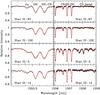 |
Fig. 5 Example of spectral synthesis in M 22: observations (black points) and synthetic spectra (red line) for the stars IV-97, IV-102, III-3, and III-14 around 1553.5 nm (left panel) and 1557.5 nm (right panel). Adopted abundances can be found in Tables 2 and 4. Some atomic and molecular lines are also indicated in the figure. |
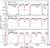 |
Fig. 7 Example of spectral synthesis for the stars IV-97 (top), IV-102 (middle), and III-3 (bottom) covering the HF, CO, and Na lines in the K band. Observed spectra (black points) are fitted by synthetic spectra (red line) whose abundances are given in Tables 2 and 4. Atomic and molecular lines are indicated. |
 |
Fig. 9 Comparison of observed (black points) and synthetic (red line) spectra for six stars in M 22 around the HF molecular line. Metallicities and fluorine abundances are indicated. The dashed blue lines in panel a) indicate variations in the best-fitting fluorine abundance by ± 0.20 dex. |
We then estimate the impact on the abundance ratios by varying the stellar parameters of ΔTeff ≈ ± 100 K, Δlog g ≈ ± 0.3 dex and Δvt ≈ 0.2 km s-1. The individual values as well as the total abundance errors due to uncertainties in the different atmospheric parameters added in quadrature are shown in Table 3.
Sensitivities in the abundance ratios for the star III-52.
4. Results and discussions
4.1. Radial velocity and cluster membership
Radial velocities were obtained using the IRAF task rvidlines in each wavelength setting by using clean isolated lines. In the H band we found a mean radial velocity of vr = −148.9 ± 0.2 (σ = 0.6,9 stars) km s-1, while in the K band it was vr = −148.9 ± 0.2 (σ = 0.5) km s-1. Additionally, our results are in excellent agreement with literature values where, for example, Harris (1996) provided a mean value of vr = −148.9 ± 0.4 km s-1. Stars III3, IV97 and III-52 were recently analyzed by Marino et al. (2009) who found mean values of vr = −148.16, − 149.84 and − 153.22 km s-1, respectively. These comparisons are an independent check that all program stars belong to M 22.
Final abundances.
4.2. Iron
The program stars have metallicities ranging from [Fe/H] = − 1.87 to − 1.44, which represent a metallicity variation of +0.43 dex (a factor higher than 2.5) in M 22 (see Table 2 Col. 8, [Fe/H]IR). Within the uncertaintites, this metallicity spread is in very good agreement with previous values based on lower resolution optical data (e.g. Pilachowski et al. 1982), and it is ~0.10 dex higher than the value found by Marino et al. (2009) using high resolution optical spectra. In Fig. 10 we compare our metallicities to those of Marino et al. (2009). For the nine stars in commom, we find that our mean [Fe/H] is higher by +0.13 ± 0.02 (σ = 0.05). Interestingly, while Marino et al. (2011) argue that the spread in [Fe/H] is lower than that observed in [Ca/H], our data show that the spread in [Fe/H] (+0.43 dex) is actually about the same as the spread in [Ca/H] (+0.47 dex) obtained in the optical.
We note from Table 3 that the total error in [Fe/H] is about 0.04 dex, while Marino et al. (2011) estimate a total error in [Fe/H] of about 0.10 ± 0.02 dex using optical FeI lines (see their Table 4). This difference is due to the weaker sensitivity to Teff of FeI lines with high excitation potential in the infrared. Indeed, the optical spectroscopic Teff is mainly determined by the sensitivity to Teff of FeI lines with low excitation potential. Even though there are only a few FeI lines in the H band, they are less sensitive to variations in the stellar parameters. We thus confirm that there is an intrinsic metallicity dispersion in M 22 as high as ~0.4 dex. Such a large [Fe/H]-dispersion is not seen in mono-metallic GCs but it is still smaller than the dispersion found in the complex GC ω Cen (see, e.g. Da Costa et al. 2009, for a detailed discussion).
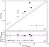 |
Fig. 10 a) Comparison of spectroscopic metallicities obtained in the infrared (this work) versus in the optical (Marino et al. 2009) for s-poor (open circles) and s-rich (filled circles) stars. Typical uncertainties are shown.b) [Fe/H] residuals (ours minus optical values), where the dashed lines represent 1σ scatter over the mean value found (full line). |
In addition, Da Costa et al. (2009) obtained intermediate resolution spectra at the Ca II triplet for 41 M 22 member red giant stars. They found that the observed M 22 [Fe/H]-distribution peaks at [Fe/H] = − 1.90 dex, with their highest abundance star presenting [Fe/H] = –1.45. Although we have no stars in common with Da Costa et al. (2009), we note that our recovered metallicities agree very well with the observed M 22 [Fe/H]-distribution presented in Da Costa et al. (2009).
For M 22, Brown & Wallerstein (1992) were the first to show that its CN-weak, CN-strong dichotomy was also accompanied by a dichotomy in [Fe/H] and [s/Fe] (see, e.g., their Table 5). In their analysis, the CN-weak group has ⟨ [Fe/H] ⟩ = −1.76 and ⟨ [Ba/Fe] ⟩ = 0.05, whereas the CN-strong group shows ⟨ [Fe/H] ⟩ = −1.57 and ⟨ [Ba/Fe] ⟩ = 0.48. These results were recently confirmed by Marino et al. (2011) using a larger high quality sample of stars. In Table 4 we list the final abundances derived in this work along with the mean [s/Fe] for each individual star, where s stands for Ba and La taken from Marino et al. (2011). Using our [Fe/H]IR values, we find that the [s/Fe]-poor group has ⟨ [Fe/H] ⟩ = −1.72 ± 0.04 (σ = 0.11, N = 6 stars), whereas the [s/Fe]-rich group presents ⟨ [Fe/H] ⟩ = −1.53 ± 0.05 (σ = 0.09,N = 3 stars). We conclude that our results are in agreement with those presented in Kayser et al. (2008) who found that the number of CN-weak stars in M 22 exceeds the number of CN-strong ones. Also, even though we are dealing with a limited sample of stars, the results presented in Fig. 10 suggest that both s-poor and s-rich groups overlap in [Fe/H].
4.3. Carbon, nitrogen, oxygen and sodium
In Fig. 11 the [(N,O,Na)/Fe] abundance ratios are plotted as a function of [C/Fe]. For all stars analyzed, the [C/Fe] abundance ratios range from − 1.01 to –0.01 while [N/Fe] varies from +0.43 to 1.33. As shown in Fig. 11a, the s-poor stars (open circles), with [C/Fe] lower than –0.7, present a spread in [N/Fe] of 0.8, which is accompanied by a small variation (~0.3 dex) in [C/Fe]. On the other hand, the s-rich stars (filled circles), with [C/Fe] higher than –0.3, present slightly the same variation in [C/Fe] (~0.3 dex) that is accompanied by a smaller spread in [N/Fe] (~0.4). These outcomes are in good agreement with previous results (see, e.g., Brown et al. 1990; Marino et al. 2011).
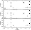 |
Fig. 11 [N/Fe], [O/Fe], and [Na/Fe] as a function of [C/Fe] for the s-poor (open circles) and s-rich (filled circles) stars. Typical uncertainties are shown. |
For oxygen, we also estimate a large abundance spread that ranges from [O/Fe] = 0.01 to 0.76. These values are in good agreement ( ≲ 1σ) with the analysis performed in the optical by Marino et al. (2011) using the forbidden [OI] line at 630 nm. However, the star III-3 in our analysis presents [O/Fe] that is higher by 0.35 dex than the mean value found by Marino et al. (2011), ⟨ [O/Fe] ⟩ = 0.41 ± 0.15. We do not seek to understand the origin of this difference. Interestingly, M 22 follows the same high [O/Fe] dispersion presented by ω Cen at the same [Fe/H] range (e.g. Johnson & Pilachowski 2010). Alternatively, Brown et al. (1990) found a spread of +0.10 dex in [O/Fe] when an extra reddening is applied to the sample; however, this spread increases to +0.30 dex if a uniform reddening is assumed. Thus, except for one star, we find that the α-element O is overabundant relative to Fe with values similar to those seen in halo metal-poor stars. These O overabundances indicate a rapid chemical evolution history dominated by Type II Supernovae.
Within the limited sample and taking into account the uncertainty of the measurements, Figs. 11a,b show that even though some s-poor giants have [N/Fe] and [O/Fe] abundances as high as those of at least two of the s-rich giants, the average [(N,O)/Fe] abundances in the s-poor M 22 stars are lower than in the s-rich group. Sodium, however, spans a larger amplitude abundance in the s-poor stars compared to the s-rich group (see Fig. 11c).
We find a mean ⟨ A(C+N+O) ⟩ = 7.68 ± 0.25 (N = 9 stars), with a large amplitude abundance of ~0.7 dex (~3σ). From the optical analysis, Marino et al. (2011) found ⟨ A(C+N+O) ⟩ = 7.68 ± 0.16 (N = 14 stars) for this GC, whereas Brown & Wallerstein (1992) found ⟨ A(C+N+O) ⟩ = 8.04 ± 0.24 (N = 7 stars). If we consider the s-rich and s-poor group separately, we find ⟨ A(C+N+O) ⟩ = 7.93 ± 0.08 (σ = 0.13,N = 3 stars) and ⟨ A(C+N+O) ⟩ = 7.55 ± 0.08 (σ = 0.19,N = 6 stars) for the s-rich and s-poor groups, respectively. From the optical analysis, Marino et al. (2011) estimated that the s-poor group star has ⟨ A(C+N+O) ⟩ = 7.57 ± 0.03 (σ = 0.09), whereas the s-rich group displays ⟨ A(C+N+O) ⟩ = 7.84 ± 0.03 (σ = 0.07). These results imply that even though M 22 presents a large amplitude variation in its total A(C+N+O) abundance, within of each M 22 s-process group the sum A(C+N+O) is constant. For our sample, ⟨ A(C+N+O) ⟩ s − poor is smaller than ⟨ A(C+N+O) ⟩ s − rich by ~0.40 dex, which confirms the results presented by Marino et al. (2011).
For mono-metallic GCs that were also analyzed in the infrared, Smith et al. (2005) found ⟨ A(C+N+O) ⟩ = 8.16 ± 0.08 for M 4, while Yong et al. (2008) found ⟨ A(C+N+O) ⟩ = 8.39 ± 0.14 for NGC 6712. Both GCs present abundance amplitude of A(C+N+O) lower than 0.35 dex. Alternatively, for NGC 1851, another GC displaying multiple stellar populations, a large 0.6 dex range in A(C+N+O) was also found by Yong et al. (2009) analysing high quality optical data of four giant stars. However, Villanova et al. (2010) recently claimed to find no significant A(C+N+O) variation in this GC. While the observed discrepancies in the CNO abundance pattern of NGC 1851 need to be understood, theoretical models (e.g. Cassisi et al. 2008) suggested that the total A(C+N+O) abundance in NGC 1851 should be increased by a factor of 2 to better understand the multiple stellar populations. A(C+N+O) also varies among the different [Fe/H] stellar groups of ω Cen (see, e.g., Marino et al. 2012). The large abundance spreads we recover for C, N and O might be intrinsically related to the complex nucleosynthetic history of M 22.
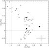 |
Fig. 12 [O/Fe] vs. [Na/Fe] from this study (open and closed circles) and from Marino et al. (2011) (crosses). Open and closed circles represent s-poor and s-rich stars, respectively. Typical error bars are indicated. |
Using Hubble Space Telescope images, Piotto (2009) found evidence for a double sub-giant branch (SGB) for M 22 which requires a complex star formation history. While the metallicity spread itself would not explain these two different stellar populations, the M 22’s large A(C+N+O) abundance spread we recover on the RGB could play a key role if it is also acting on the SGB. We recall that at least for NGC 1851, abundance variations in A(C+N+O) have been advocated to explain the different stellar populations (Cassisi et al. 2008).
In Fig. 12 we plot [O/Fe] against [Na/Fe] for eight out of nine stars. For comparison, we also added in this figure the abundances obtained in the optical by Marino et al. (2011) for a larger sample. As seen in this figure, both s-rich and s-poor stars in M 22 present mean [O/Fe] around 0.40 dex accompanied by a high Na variation (–0.23 ≤ [Na/Fe] ≤ 0.51). In line with the results found by Marino et al. (2011), while our three s-rich stars present [Na/Fe] > 0, the five s-poor stars range from low ([Na/Fe] < 0) to high (0.10 < [Na/Fe] ≤ 0.51) Na abundances. As noted by the referee, the apparent turnover in Fig. 12 (see also Fig. 14 of Marino et al. 2011) is possibly due to the small sample statistics in the case of s-poor giant stars with [Na/Fe] < 0. At such low Na abundances the Na-O relation seems to become very steep and, consequently, there is a substantial change in [Na/Fe] over a small change in oxygen around [O/Fe] ~ 0.40 dex. The Na abundance scatter in such a near-vertical Na-O relation might artificially produce the visual impression of a correlation between Na-O at [Na/Fe] < 0. Thus, our independent analysis at infrared wavelengths also reveals the well-known Na-O anticorrelation operating in Galactic GCs, which originates from the enrichment of high-temperature H-burning processed material from the CNO cycle and NeNa chain.
4.4. Fluorine
To date, F has only been investigated in a small number of stars in three GCs: ω Cen (Cunha et al. 2003, 2 stars), M 4 (Smith et al. 2005, 7 stars) and NGC 6712 (Yong et al. 2008, 5 stars). For M 4 and NGC 6712, the GCs with more than two stars with F measurements, the data reveal that fluorine presents the largest star-to-star abundance amplitude of all elements and that it is correlated with other light elements. Therefore, understanding the behavior of F is critical for understanding the chemical abundance anomalies in GCs.
For M 22, we obtained F abundances for seven out of nine stars. A(F) abundances range from 2.82 to 3.12, which correspond to –0.20 ≤ [F/Fe] ≤ +0.28 or –0.86 ≤ [F/O] ≤ +0.27. We stress, however, that for stars III-14 and III-12 we have obtained only the upper limits of their F abundances due to the weak features of the HF lines (see Figs. 8 and 9). In contrast to what is seen in M 4 and NGC 6712, the amplitude of the A(O) variation in M 22 is slightly larger than that of A(F).
As noted, in M 4 and NGC 6712 the abundance of F was correlated with the abundance of other light elements, C, N, O, and Na, and these correlations were significant. For M 22, when we compare the A(F) abundance with A(C, N, O, Na), we do not find any significant correlations. Therefore, despite the fact that there is a large F abundance variation in M 22, unlike M 4 and NGC 6712 there are no significant correlations between F and the other light elements. The absence of such correlations may be attributed to the small sample size and/or the more complex chemical enrichment history of M 22 relative to the mono-metallic clusters M 4 and NGC 6712.
Yong et al. (2008) noted that GCs and field stars seem to define different trends in the A(F)- and [F/O]-A(O) planes, which is in agreement with the general finding that GCs have abundance patterns that are distinct from those of the field (see Gratton et al. 2004, for a review). A given globular cluster contains stars with O abundances spanning a large range of values. The upper envelope of these values is in accord with field stars at the same metallicity while the lower envelope extends down to stars whose O has been depleted by a factor of 10 or more. Similarly, the F abundances show star-to-star variations in which the F and O abundances are correlated such that the most F-rich objects are also the most O-rich. Thus, in the limited data, Yong et al. (2008) showed that the [F/O] ratio is constant in a given GC. They detected a linear decrease of A(F) with A(O), accompanied by a constant [F/O] ratio as the A(O) abundances decrease, which suggests that the nucleosynthetic process(es) responsible for the light element abundance variations deplete F and O by the same amounts. If this is the case, the [F/O] discrepancy between field stars and GCs is likely driven by unusually low F abundances in GCs relative to field stars.
Following Yong et al. (2008), we show in Fig. 13 the abundances of A(F) and log[n(F)/n(O)] against A(O) for M 22 compared with those values in different stellar components and environments (field and GCs), as indicated in the figure’s caption. Looking at the M 22 sample as a whole, the main conclusion is that A(F) remains nearly constant with A(O), with ⟨ A(F) ⟩ = 2.89 ± 0.07 (σ = 0.20 dex, N = 7 stars), whereas the F/O abundance drastically increases for A(O) abundances lower than 7.5 dex. Rejecting the upper limits on F, the average A(F) for the s-rich stars is ⟨ A(F) ⟩ = 2.88 ± 0.06 (σ = 0.08 dex, N = 2 stars), while for the s-poor stars ⟨ A(F) ⟩ = 2.98 ± 0.08 (σ = 0.14 dex, N = 3 stars). Within the limited data, the s-poor sample has a larger F abundance dispersion than the s-rich sample. However, within the uncertainties, the two populations have the same mean A(F).
On the other hand, a detailed inspection of Fig. 13 suggests that for our limited number of stars in M 22, the sample is well divided at A(O) = 7.5 dex. In this figure, the stars III-15, IV-97 and IV-102 have the lowest A(O) abundances or [O/Fe] = (+0.01, +0.36, +0.41), which are in good agreement with those found by Marino et al. (2011), that is, [O/Fe] = (+0.11, +0.40, +0.43), respectively. In addition, as seen in Figs. 7–9, the HF features in these three stars are relatively strong, implying that their F abundances are not upper limits. Thus, whether one subdivides the sample based on their A(O) metallicities, four M 22 member giant stars (3 s-rich and 1 s-poor) follow the general linear A(F)-A(O) trend found by Yong et al. (2008) for three Galactic GCs, albeit with a higher dispersion. Additional F measurements of more metal-poor field and GC stars are required in order to draw firm conclusions about the Galactic A(F)-A(O) at low metallicities.
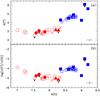 |
Fig. 13 a) A(F) vs. A(O) and b) log[n(F)/n(O)] vs. A(O). Symbols stand for: s-rich M 22 stars (filled circles), s-poor M 22 stars (open circles), NGC 6712 (crosses: Yong et al. 2008), M 4 (open squares: Smith et al. 2005), ω Cen (filled triangles: Cunha et al. 2003), bulge stars (filled squares: Cunha et al. 2008), and field stars (stars: Cunha et al. 2003; Cunha & Smith 2005). |
In Fig. 14 we show the F and Na-O abundance diagram in M 22 compared to that seen in ω Cen, M 4 and NGC 6712. Overall, there is a general trend for [F/Fe] to increase with [O/Fe] and decrease with [Na/Fe] in the different GCs. Once again, an intriguing feature of this figure concerns the location of the three stars with the lowest A(O) abundances in M 22. Within the observed uncertainties, the stars IV-97 and IV-102 do follow the global [F/Fe]-[O/Fe]:[Na/Fe] trend at [O/Fe] ~ 0.40. However, the most F-rich ([F/Fe] = +0.28), O-depleted ([O/Fe] = +0.01), and Na-rich ([Na/Fe] = +0.51) star in M 22, III-15, clearly does not follow this general trend. Instead, the observed [F/Fe] abundance ratio of the star III-15 differs by more than 1 dex with respect to what is observed for NGC 6712 at nearly the same [O/Fe] ratio. This result is very intriguing with no easy explanation as III-15 is confirmed kinematically and spectroscopically as a M 22 member.
As discussed in Kobayashi et al. (2011) both the ν-process of core-collapse supernovae (SNe II and HNe) and AGB stars play a crucial role in the production of F. Nevertheless, the relative contribution from low-mass supernovae may be smaller in the GCs than in the field. F production in AGB stars is dominated by the contribution of stars with masses ≈ 1–3 M⊙, depending on metallicity (see also the yields of Karakas 2010). For these stars, the abundances of C and F need to be considered together with the s-process elements because the F production in AGB stars occurs in the He-intershell via a complex series of proton, α, and neutron-capture reactions, beginning with the 14N(α,γ)18F(β+)18O(p, α)15N(α,γ)19F reaction. The protons for the CNO cycle reaction 18O(p, α)15N come from the 14N(n, p)14C reaction, which in turn requires free neutrons. The dominant neutron source in low-mass AGB stars for F and s-process element production is the 13C(α, n)O16 reaction (e.g., Busso et al. 2001). Furthermore, because F production occurs in the He-intershell, it is dredged to the surface via the repeated action of the third dredge-up (TDU), along with C and any s-process elements.
It is important to remember that the lifetimes of AGB stars with M ≲ 3 M⊙ are relatively long (τ ≳ 300 Myr). It is not clear if these stars will have had time to contribute toward the bulk chemical enrichment of a forming GC, which show no discernible age spread (see e.g. Marín-Franch et al. 2009). It is partly for this reason that the contribution of intermediate-mass AGB stars, with masses between 4–8 M⊙, is so attractive. In intermediate-mass AGB stars, the base of the convective envelope can reach the top of the H-burning shell, causing proton-capture nucleosynthesis to occur there (known as hot bottom burning, HBB). The main result is that CNO nuclei are converted into N, and F is efficiently destroyed. One of the biggest uncertainties to effect models of intermediate-mass AGB stars is the unknown efficiency of the TDU. At low metallicity, theoretical models predict either no or little TDU (Ventura & D’Antona 2009) or predict that intermediate-mass AGB stars experience efficient TDU (Herwig 2004; Karakas 2010). Models with efficient TDU would also produce s-process elements via the 22Ne(α, n)Mg25 neutron source that operates during convective thermal pulses. The main signature would be copious production of elements near the first s-process peak (e.g., Rb, Sr, Y, Zr) and much smaller quantities of Ba and Pb (e.g., the metallicity Fe/H = − 2.3 models of Lugaro et al. 2011). One implication of an efficient TDU is that the total number of C+N+O nuclei is not conserved.
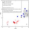 |
Fig. 15 A(F) vs. A(C) for different objects in the Galaxy. Symbols stand for: s-rich M 22 stars (filled circles), s-poor M 22 stars (open circles), NGC 6712 (crosses: Yong et al. 2008), M 4 (open squares: Smith et al. 2005), bulge stars (filled squares: Cunha et al. 2008), Ba star (filled triangle: Alves-Brito et al. 2011), Orion giant stars (open triangles: Cunha & Smith 2005; Cunha et al. 2008), CEMP and AGB stars (stars: Schuler et al. 2007; Abia et al. 2009). The hachured area indicates the A(F)-A(C) position of Galactic AGB stars analyzed in Abia et al. (2010). |
In Fig. 15, which shows A(F) as a function of A(C), we find further evidence for the chemical dissimilarity between F abundances in the field from those of GCs. Interestingly, all field giant stars analyzed (regardless of their [C/Fe]-enhancements) have higher A(F) abundances than those of GCs. We note, however, that there is no overlap in [Fe/H] between the field and GC stars. Within the limited sample, the M 22 C- and s-rich population shares a similar A(F)-A(C) relation compared to the stars analyzed in other GCs. On the other hand, the M 22 C- and s-poor population does not fit the general linear A(F)-A(C) trend seen for the other GCs. We would like to reinforce once again that the three comparison GCs for which F data are available are all more oxygen-rich than the A(O)-poorest giants in the M 22 sample. Hence, the significance of the non-linearity in the M 22 A(O)-A(F) data at low abundances is still unclear. Additional F data for other low-metallicity GCs are required to determine whether the A(O)-A(F) relation in M 22 is unusual as a result of its complex nucleosynthetic history or, alternatively, whether the GC population in general shows a non-linear A(O)-A(F) relation at low [Fe/H].
Figure 16 displays [F/O] against the mean [(s-process)/Fe]. From this figure, there is evidence for an anticorrelation between the [F/O] and s-process enhancements in GCs in the sense that s-rich stars also have lower [F/O] abundances. In the solar system, the main component of the s-process contributes to about 84% of the Ba abundances, whereas ≈ 16% is due to the r-process (see, e.g. Travaglio et al. 1999); for La, this proportion is of 61% (s) and 39% (r). While the r-process is related to the final stages of evolution of massive stars (M > 8 M⊙), the s-process main component is believed to occur in AGB stars of low (1–3 M⊙) or intermediate (4–8 M⊙) masses (see, e.g. Busso et al. 1999). However, as noted above, the production of s-process elements in intermediate-mass AGB stars is accompanied by F destruction and could account for the anti-correlation seen in Fig. 16. Theoretical predictions of s-process nucleosynthesis from intermediate-mass AGB stars at the metallicities of M 22 are needed to verify this scenario.
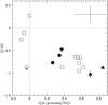 |
Fig. 16 [F/O] vs. ⟨ [(s-process)/Fe] ⟩ for s-rich M 22 stars (filled circles), s-poor M 22 stars (open circles), M 4 (open squares: Smith et al. 2005), and ω Cen (filled triangles: Cunha et al. 2003). |
For NGC 6712, Yong et al. (2008) found that its [F/O] abundance amplitude is compatible with a production in massive (M ≳ 5 M⊙) AGB stars. Unfortunately, there are no observational clues about the s-process enrichment in NGC 6712. For M 4, not only its high s-process enrichment (Ivans et al. 1999) but also its [F/O] abundance ratio (Smith et al. 2005) suggest a chemical enrichment history dominated by intermediate AGB stars.
M 22 and ω Cen, however, present discrete stellar populations in their CMDs, which means they have experienced a more complex nucleosynthetic history. For ω Cen, Cunha et al. (2003) argue that the low [F/O] abundances obtained for two s-rich stars cannot be explained by the production of F as the result of low-mass metal-poor AGB stars. M 22, on the one hand, presents a sharp separation between its s-rich and s-poor groups, which can be explained in terms of its double stellar populations (Marino et al. 2009). After testing different chemical models to explain the observed [F/O] abundances in all GCs studied to date (including our preliminary results), Kobayashi et al. (2011) showed that the observed [F/O] abundances in GCs are consistent with models that include the AGB yields only. However, given the timescale considerations noted above, an alternative scenario might be to consider a small contribution from SNe in GC (these produce F via the ν process) followed by the destruction of F via HBB in intermediate-mass AGB stars. These AGB stars have also produced s-process elements along with large amounts of helium (see discussion in Roederer et al. 2011). Norris (2004) claims that massive stars could be the source of the high helium necessary to explain the different stellar populations on the main sequence of ω Cen. As M 22 shares chemical properties with ω Cen, this explanation could also, in principle, be extended to M 22.
5. Conclusions
We have acquired high-resolution infrared data for a sample of nine stars in the Galactic globular cluster M 22. The main goal was to obtain high precision abundances of C, N, O, F, Na and Fe using atomic and molecular lines in the H and K bands.
We confirm with high quality data at infrared wavelengths that M 22 resembles the chemical properties seen not only in mono-metallic GCs but also in other massive GCs displaying multiple stellar populations. We have found/confirmed that:
-
There is a spread in [Fe/H] in M 22 of ~0.4 dex.
-
There is a large dispersion in the light C, N, and O elements. Although A(C+N+O) spans a large amplitude abundance (~0.7 dex), it is approximately constant within each M 22 s-process group.
-
O and Na are anticorrelated.
-
The abundance spread for F is ΔA(F) = 0.6 dex, an amplitude comparable to that seen for other light elements in M 22.
-
While the four most A(O)-rich stars are consistent with the general linear A(F)-A(O) trend from other Galactic GCs, the three most A(O)-poor stars in M 22 do not follow this trend. More data at low metallicity are required.
IRAF is distributed by the National Optical Astronomy Observatory, which is operated by the Association of Universities for Research in Astronomy (AURA) under cooperative agreement with the National Science Foundation.
In this work we used the standard spectroscopic notation A(X) = log[n(X)/n(H)] +12 and [X/Y] = log[n(X)/n(Y)]∗ – log[n(X)/n(Y)]⊙.
Acknowledgments
A.A.B. acknowledges support from FONDECYT-Chile (3100013), CNPq-Brazil (PDE, 200227/2008-4), and ARC (Super Science Fellowship, FS110200016). J.M. thanks support from FAPESP (2010/50930-6), USP (Novos Docentes), and CNPq (Bolsa de produtividade). We wish to thank Dr. Stuart Ryder, from the Australian Gemini Office, for his assistance during the Phase II definitions of our Gemini/Phoenix observations, and also Dr. Javier Alonso-Garcia for providing us Fig. 2. We warmly thank Prof Gary da Costa for reading the manuscript and for his helpful comments and remarks. We also thank the anonymous referee for helping improving the paper. Based on observations obtained at the Gemini Observatory, which is operated by the AURA, Inc., under a cooperative agreement with the NSF on behalf of the Geminipartnership: the NSF (United States), the STFC (United Kingdom), the NRC (Canada), CONICYT (Chile), the ARC (Australia), CNPq (Brazil) and SECYT (Argentina). This paper uses data obtained with the Phoenix infrared spectrograph, developed and operated by the National Optical Astronomy Observatory. The spectra were obtained as part of the program GS-2009A-Q-26. This publication makes use of data products from the Two Mass Micron All Sky Survey, which is a joint project of the University of Massachusetts and the Infrared Processing and Analysis Center/California Institute of Technology, funded by the National Aeronautics and Space Administration and the National Science Foundation.
References
- Abia, C., Recio-Blanco, A., de Laverny, P., et al. 2009, ApJ, 694, 971 [NASA ADS] [CrossRef] [Google Scholar]
- Abia, C., Cunha, K., Cristallo, S., et al. 2010, ApJ, 715, L94 [NASA ADS] [CrossRef] [Google Scholar]
- Alves-Brito, A., Karakas, A., Yong, D., Meléndez, J., & Vásquez, S. 2011, A&A, 536, A40 [NASA ADS] [CrossRef] [EDP Sciences] [Google Scholar]
- Alonso, A., Arribas, S., & Martinez-Roger, C. 1998, A&AS, 131, 209 [NASA ADS] [CrossRef] [EDP Sciences] [Google Scholar]
- Alonso, A., Arribas, S., & Martínez-Roger, C. 1999, A&AS, 140, 261 [NASA ADS] [CrossRef] [EDP Sciences] [Google Scholar]
- Alonso-Garcia, J., Mateo, M., Sen, B., Banerjee, M., & von Braun, K. 2011, AJ, 141, 146 [NASA ADS] [CrossRef] [Google Scholar]
- Alonso-Garcia, J., Mateo, M., Sen, B., et al. 2012, AJ, 143, 70 [NASA ADS] [CrossRef] [Google Scholar]
- Anthony-Twarog, B. J., Twarog, B. A., & Craig, J. 1995, PASP, 107, 32 [NASA ADS] [CrossRef] [Google Scholar]
- Brown, J. A., & Wallerstein, G. 1992, AJ, 104, 1818 [NASA ADS] [CrossRef] [Google Scholar]
- Brown, J. A., Wallerstein, G., & Oke, J. B. 1990, AJ, 100, 1561 [NASA ADS] [CrossRef] [Google Scholar]
- Busso, M., Gallino, R., & Wasserburg, G. J. 1999, ARA&A, 37, 239 [NASA ADS] [CrossRef] [Google Scholar]
- Busso, M., Gallino, R., Lambert, D. L., Travaglio, C., & Smith, V. V. 2001, ApJ, 557, 802 [NASA ADS] [CrossRef] [Google Scholar]
- Cannon, R. D., Croke, B. F. W., Bell, R. A., Hesser, J. E., & Stathakis, R. A. 1998, MNRAS, 298, 601 [NASA ADS] [CrossRef] [Google Scholar]
- Carpenter, J. M. 2001, AJ, 121, 2851 [NASA ADS] [CrossRef] [Google Scholar]
- Cassisi, S., Salaris, M., Pietrinferni, A., et al. 2008, ApJ, 672, 115 [Google Scholar]
- Castelli, F., Gratton, R. G., & Kurucz, R. L. 1997, A&A, 318, 841 [NASA ADS] [Google Scholar]
- Cohen, J. 1981, ApJ, 247, 869 [NASA ADS] [CrossRef] [Google Scholar]
- Crocker, D. A. 1988, AJ, 96, 1649 [NASA ADS] [CrossRef] [Google Scholar]
- Cunha, K., & Smith, V. V. 2005, ApJ, 626, 425 [NASA ADS] [CrossRef] [Google Scholar]
- Cunha, K., Smith, V. V., Lambert, D. L., & Hinkle, K. H. 2003, AJ, 126, 1305 [NASA ADS] [CrossRef] [Google Scholar]
- Cunha, K., Smith, V. V., & Gibson, B. K. 2008, ApJ, 679, L17 [NASA ADS] [CrossRef] [Google Scholar]
- Da Costa, G. S., Held, E.V., Saviane, I., & Gullieuszik, M. 2009, ApJ, 705, 1481 [NASA ADS] [CrossRef] [Google Scholar]
- Frogel, J. A., Cohen, J. G., & Persson, S. E. 1983, ApJS, 53, 713 [NASA ADS] [CrossRef] [Google Scholar]
- Gratton, R. 1982, A&A, 115, 171 [NASA ADS] [Google Scholar]
- Gratton, R., Sneden, C., & Carretta, E. 2004, ARA&A, 42, 385 [NASA ADS] [CrossRef] [Google Scholar]
- Harris, B. W. 1996, AJ, 112, 1487 [NASA ADS] [CrossRef] [Google Scholar]
- Herwig, F. 2004, ApJS, 155, 651 [NASA ADS] [CrossRef] [Google Scholar]
- Hesser, J. E., & Harris, G. L. H. 1979, ApJ, 234, 513 [NASA ADS] [CrossRef] [Google Scholar]
- Hesser, J. E., Hartwick, F. D. A., & McClure, R. D. 1977, ApJS, 33, 471 [NASA ADS] [CrossRef] [Google Scholar]
- Hinkle, K. H., Blum, R. D., Joyce, R. R., et al. 2003, in SPIE Conf. Ser. 4834, ed. P. Guhathakurta, 353 [Google Scholar]
- Ivans, I. I., Sneden, C., Kraft, R. P., et al. 1999, AJ, 118, 1273 [NASA ADS] [CrossRef] [Google Scholar]
- Ivans, I. I., Sneden, C., Wallerstein, G., et al. 2004, MmSAI, 75, 286 [Google Scholar]
- Johnson, C. I., & Pilachowski, C.A. 2010, ApJ, 722, 1373 [NASA ADS] [CrossRef] [Google Scholar]
- Jorissen, A., Smith, V. V., & Lambert, D. L. 1992, A&A, 261, 164 [NASA ADS] [Google Scholar]
- Karakas, A. I. 2010, MNRAS, 403, 1413 [NASA ADS] [CrossRef] [Google Scholar]
- Kayser, A., Hilker, M., Grebel, E. K., & Willemsen, P. G. 2008, A&A, 486, 437 [NASA ADS] [CrossRef] [EDP Sciences] [Google Scholar]
- Kobayashi, C., Izutani, N., Karakas, A., et al. 2011, ApJ, 739, L57 [NASA ADS] [CrossRef] [Google Scholar]
- Lehnert, M. D., Bell, R. A., & Cohen, J. G. 1991, ApJ, 367, 514 [NASA ADS] [CrossRef] [Google Scholar]
- Lugaro, M., Ugalde, C., Karakas, A. I., et al. 2004, ApJ, 615, 934 [NASA ADS] [CrossRef] [Google Scholar]
- Lugaro, M., Karakas, A. I., Stancliffe, R. J., & Rijs, C. 2011, ApJ, submitted [Google Scholar]
- Marín-Franch, A., Aparicio, A., Piotto, G., et al. 2009, ApJ, 694, 1498 [NASA ADS] [CrossRef] [Google Scholar]
- Marino, A. F., Milone, A. P., Piotto, G., et al. 2009, A&A, 505, 1099 [NASA ADS] [CrossRef] [EDP Sciences] [Google Scholar]
- Marino, A. F., Sneden, R., Kraft, R. P., et al. 2011, A&A, 532, A8 [NASA ADS] [CrossRef] [EDP Sciences] [Google Scholar]
- Marino, A. F., Milone, A. P., Piotto, G., et al. 2012, ApJ, 746, 14 [NASA ADS] [CrossRef] [Google Scholar]
- Meléndez, J., Barbuy, B., Bica, E., et al. 2003, A&A, 411, 417 [NASA ADS] [CrossRef] [EDP Sciences] [Google Scholar]
- Meléndez, J., Asplund, M., Alves-Brito, A., et al. 2008, A&A, 484, L21 [NASA ADS] [CrossRef] [EDP Sciences] [MathSciNet] [Google Scholar]
- Minitti, D., Coyne, G. V., & Claria, J. J. 1992, AJ, 103, 871 [NASA ADS] [CrossRef] [Google Scholar]
- Monaco, L., Pancino, E., Ferraro, F. R., & Bellazzini, M. 2004, MNRAS, 349, 1278 [NASA ADS] [CrossRef] [Google Scholar]
- Norris, J. E. 2004, ApJ, 612, 25 [Google Scholar]
- Norris, J., & Freeman, K. C. 1983, ApJ, 266, 130 [NASA ADS] [CrossRef] [Google Scholar]
- Peterson, R., & Cudworth, K. M. 1994, ApJ, 420, 612 [NASA ADS] [CrossRef] [Google Scholar]
- Pilachowski, C., Leep, E. M., Wallerstein, G., & Peterson, R. C. 1982, ApJ, 263, 187 [Google Scholar]
- Piotto, G., 2009, in The Ages of Stars, Proc. IAU Symp., 258, 233 [Google Scholar]
- Renzini, A., & Buzzoni, A. 1986, in Spectral Evolution of Galaxies, ed. C. Chiosi, & A. Renzini, Astrophys. Space Sci. Lib., 122, 195 [Google Scholar]
- Rieke, G. H., & Lebofsky, M. J. 1985, ApJ, 288, 618 [NASA ADS] [CrossRef] [Google Scholar]
- Roederer, I. U., Marino, A. F., & Sneden, C. 2011, ApJ, 742, 37 [Google Scholar]
- Schuler, S. C., Cunha, K., Smith, V. V., et al. 2007, ApJ, 667, L81 [NASA ADS] [CrossRef] [Google Scholar]
- Skrutskie, M. F., Cutri, R. M., Stiening, R., Weinberg, M. D., & Schneider, S. 2006, AJ, 131, 1163 [NASA ADS] [CrossRef] [Google Scholar]
- Smith, V. V., & Suntzeff, N. B. 1989, AJ, 97, 1699 [NASA ADS] [CrossRef] [Google Scholar]
- Smith, V. V., Hinkle, K. H., Cunha, K., et al. 2002, AJ, 124, 324 [Google Scholar]
- Smith, V. V., Cunha, K., Ivans, I. I., et al. 2005, ApJ, 633, 392 [NASA ADS] [CrossRef] [Google Scholar]
- Sneden, C. A. 1973, Ph.D. Thesis, University of Texas at Austin [Google Scholar]
- Travaglio, C., Galli, D., Gallino, R., et al. 1999, ApJ, 521, 691 [NASA ADS] [CrossRef] [Google Scholar]
- Valcarce, A. A. R., & Catelan, M. 2011, A&A, 533, A120 [NASA ADS] [CrossRef] [EDP Sciences] [Google Scholar]
- Ventura, P., & D’Antona, F. 2009, A&A, 499, 835 [NASA ADS] [CrossRef] [EDP Sciences] [Google Scholar]
- Villanova, S., Geisler, D., & Piotto, G. 2010, ApJ, 722, 18 [Google Scholar]
- Wallerstein, G., Leep, E. M., & Oke, J. B. 1987, AJ, 93, 1137 [NASA ADS] [CrossRef] [Google Scholar]
- Yong, D., Meléndez, J., Cunha, K., et al. 2008, ApJ, 689, 1020 [NASA ADS] [CrossRef] [Google Scholar]
- Yong, D., Grundahl, F., D’Antona, F., et al. 2009, ApJ, 695, 62 [Google Scholar]
All Tables
All Figures
|
Fig. 1 The finding chart of M 22 from the optical Digitized Sky Survey. The targets are clearly marked following the nomenclature defined in Peterson & Cudworth (1994). The field’s orientation is shown and the displayed sky area is of 15 × 15 arcmin2. The coordinates (J2000) of the image center are |
| In the text | |
|
Fig. 2 Extinction map for M 22 in equatorial coordinates (J2000). The small and large circles indicate, respectively, the GC’s center and the area where the program stars (crosses) lie in the GC’s field. The color bar gives the excesses E(B − V) for the extinction map. The zero point is arbitrary and it is calculated by comparison with isochrones (see Alonso-Garcia et al. 2011, 2012, for more details on the techniques and methods used to create this figure). The orientation is different from Fig. 1 (North-East points to the upper right corner). |
| In the text | |
|
Fig. 3 Observed (points) and best synthetic (lines) spectra of M 22 III-52 in the H (top) and K (bottom) bands. Adopted abundances can be found in Tables 2 and 4. Several atomic and molecular lines are identified. |
| In the text | |
|
Fig. 4 Example of spectral synthesis in M 22 III-52 in the K band showing, in more details, the abundance fit for CO, F and Na lines. Atomic and molecular lines as well as the derived abundances are labeled in the figure. |
| In the text | |
|
Fig. 5 Example of spectral synthesis in M 22: observations (black points) and synthetic spectra (red line) for the stars IV-97, IV-102, III-3, and III-14 around 1553.5 nm (left panel) and 1557.5 nm (right panel). Adopted abundances can be found in Tables 2 and 4. Some atomic and molecular lines are also indicated in the figure. |
| In the text | |
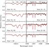 |
Fig. 6 Same as Fig. 5 but for the stars III-15, III-12, III-52 and I-92. |
| In the text | |
|
Fig. 7 Example of spectral synthesis for the stars IV-97 (top), IV-102 (middle), and III-3 (bottom) covering the HF, CO, and Na lines in the K band. Observed spectra (black points) are fitted by synthetic spectra (red line) whose abundances are given in Tables 2 and 4. Atomic and molecular lines are indicated. |
| In the text | |
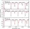 |
Fig. 8 Same as Fig. 7 but for the stars III-14, III-15 and III-12. |
| In the text | |
|
Fig. 9 Comparison of observed (black points) and synthetic (red line) spectra for six stars in M 22 around the HF molecular line. Metallicities and fluorine abundances are indicated. The dashed blue lines in panel a) indicate variations in the best-fitting fluorine abundance by ± 0.20 dex. |
| In the text | |
|
Fig. 10 a) Comparison of spectroscopic metallicities obtained in the infrared (this work) versus in the optical (Marino et al. 2009) for s-poor (open circles) and s-rich (filled circles) stars. Typical uncertainties are shown.b) [Fe/H] residuals (ours minus optical values), where the dashed lines represent 1σ scatter over the mean value found (full line). |
| In the text | |
|
Fig. 11 [N/Fe], [O/Fe], and [Na/Fe] as a function of [C/Fe] for the s-poor (open circles) and s-rich (filled circles) stars. Typical uncertainties are shown. |
| In the text | |
|
Fig. 12 [O/Fe] vs. [Na/Fe] from this study (open and closed circles) and from Marino et al. (2011) (crosses). Open and closed circles represent s-poor and s-rich stars, respectively. Typical error bars are indicated. |
| In the text | |
|
Fig. 13 a) A(F) vs. A(O) and b) log[n(F)/n(O)] vs. A(O). Symbols stand for: s-rich M 22 stars (filled circles), s-poor M 22 stars (open circles), NGC 6712 (crosses: Yong et al. 2008), M 4 (open squares: Smith et al. 2005), ω Cen (filled triangles: Cunha et al. 2003), bulge stars (filled squares: Cunha et al. 2008), and field stars (stars: Cunha et al. 2003; Cunha & Smith 2005). |
| In the text | |
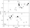 |
Fig. 14 [F/Fe] against [O/Fe] (top) and [Na/Fe] (bottom). Symbols are as given in Fig. 13. |
| In the text | |
|
Fig. 15 A(F) vs. A(C) for different objects in the Galaxy. Symbols stand for: s-rich M 22 stars (filled circles), s-poor M 22 stars (open circles), NGC 6712 (crosses: Yong et al. 2008), M 4 (open squares: Smith et al. 2005), bulge stars (filled squares: Cunha et al. 2008), Ba star (filled triangle: Alves-Brito et al. 2011), Orion giant stars (open triangles: Cunha & Smith 2005; Cunha et al. 2008), CEMP and AGB stars (stars: Schuler et al. 2007; Abia et al. 2009). The hachured area indicates the A(F)-A(C) position of Galactic AGB stars analyzed in Abia et al. (2010). |
| In the text | |
|
Fig. 16 [F/O] vs. ⟨ [(s-process)/Fe] ⟩ for s-rich M 22 stars (filled circles), s-poor M 22 stars (open circles), M 4 (open squares: Smith et al. 2005), and ω Cen (filled triangles: Cunha et al. 2003). |
| In the text | |
Current usage metrics show cumulative count of Article Views (full-text article views including HTML views, PDF and ePub downloads, according to the available data) and Abstracts Views on Vision4Press platform.
Data correspond to usage on the plateform after 2015. The current usage metrics is available 48-96 hours after online publication and is updated daily on week days.
Initial download of the metrics may take a while.