| Issue |
A&A
Volume 540, April 2012
|
|
|---|---|---|
| Article Number | A133 | |
| Number of page(s) | 119 | |
| Section | Catalogs and data | |
| DOI | https://doi.org/10.1051/0004-6361/201116696 | |
| Published online | 11 April 2012 | |
η Carinae: linelist for the emission spectrum of the Weigelt blobs in the 1700 to 10 400 Å wavelength region⋆
1 Atomic Astrophysics, Lund Observatory, Lund University, Box 43, 22100 Lund, Sweden
e-mail: This email address is being protected from spambots. You need JavaScript enabled to view it.
2 Astrophysics Science Division, Code 667, Goddard Space Flight Center, Greenbelt, MD 20771, USA
e-mail: This email address is being protected from spambots. You need JavaScript enabled to view it.
Received: 11 February 2011
Accepted: 27 January 2012
Abstract
Aims. We present line identifications in the 1700 to 10 400 Å region for the Weigelt blobs B and D, located 0″.1 to 0″.3 NNW of Eta Carinae. The aim of this work is to characterize the behavior of these luminous, dense gas blobs in response to the broad high-state and the short low-state of η Carinae during its 5.54-year spectroscopic period.
Methods. The spectra were recorded in a low state (March 1998) and an early high state (February 1999) with the Hubble Space Telescope/Space Telescope Imaging Spectrograph (HST/STIS) from 1640 to 10 400 Å using the 52″ × 0″.1 aperture centered on Eta Carinae at position angle, PA = 332 degrees. Extractions of the reduced spectrum including both Weigelt B and D, 0″.28 in length along the slit, were used to identify the narrow, nebular emission lines, measure their wavelengths and estimate their fluxes.
Results. A linelist of 2500 lines is presented for the high and low states of the combined Weigelt blobs B and D. The spectra are dominated by emission lines from the iron-group elements, but include lines from lighter elements including parity-permitted and forbidden lines. A number of lines are fluorescent lines pumped by H Lyα. Other lines show anomalous excitation.
Key words: line: identification / circumstellar matter / stars: kinematics and dynamics / stars: individual: η Carinae
Table C.1 is also available at the CDS via anonymous ftp to cdsarc.u-strasbg.fr (130.79.128.5) or via http://cdsarc.u-strasbg.fr/viz-bin/qcat?J/A+A/540/A133
Deceased.
© ESO, 2012
1. Introduction
The spectrum of the luminous blue variable (LBV) star Eta Carinae (η Car) has been complex and challenging ever since it was first recorded in the late 19th century. The first detailed spectral analyses were made in Cape Town by Thackeray (1953), who recorded the spectrum from 3700 to 8900 Å in the near-infrared, and by Gaviola (1953) in Córdoba, Argentina. Thackeray (1962, 1967) later extended the spectral region to cover from 3100 to 9100 Å. The spectrum showed a profusion of forbidden emission lines, predominantly from Fe ii, but also from ions with higher ionization stages, such as Fe iii, Ne iii and Ar iii. There were also permitted emission lines normally associated with collisional excitation or recombination. Ground-based images of the object implied that several diverse regions with presumably different plasma conditions contributed to the spectrum. In the infrared spectral region, η Car was known for its huge excess peaking at wavelengths around 10 μm (Neugebauer & Westphal 1968; Robinson et al. 1973).
The first real step forward to understand the complexity of the emission line spectrum was taken when Weigelt & Ebersberger (1986), using speckle interferometry, discovered four separated components. Component A proved to be the central source characterized by strong continuum and broad wind line profiles. The other three components, known as Weigelt blobs B, C and D, are narrow line emission structures later explained to be gas blobs ejected from the star during the lesser eruption of the 1890s (Smith et al. 2004). The great eruption of η Car occurred in the 1840s, rivaling Sirius in apparent magnitude. Each blob, being slightly extended, projects within tenths of an arcsecond from η Car and lies within lightdays of the central source.
The second major step was spectroscopic observations made with the Hubble Space Telescope (HST). Spectra, demonstrating the narrow line emission character of the Weigelt blobs, were first recorded with the Faint Object Spectrograph (FOS) (Davidson et al. 1995), then with the Goddard High Resolution Spectrograph (GHRS) (Davidson et al. 1997). While the small circular apertures, coupled with the initial spherical aberration, prevented complete isolation of η Car from the Weigelt blobs, small offsets in position demonstrated their nebular character. Clear spatial and spectral separation of the Weigelt blobs finally was achieved with the Space Telescope Imaging Spectrograph (STIS) (Gull et al. 1999). The relay-optics-corrected spatial resolution of HST, 0 1 at visible wavelengths, makes it extremely suitable for detailed spectroscopy of the blobs well separated from the central source. The 52″ × 01 aperture of the STIS instrument, at appropriate position angles, simultaneously provided spatially-resolved spectra of η Car and selected Weigelt blobs.
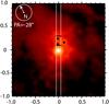 |
Fig. 1 Weigelt blobs B and D: taken from an HST/ACS F550M image recorded in 2002, the 2″ × 2″ field of view reveals the complex ejecta surrounding η Car (white core). Three dots define the positions of Weigelt blobs B, C and D. Superimposed (white lines) is the position of the HST/STIS 52″ × 0 |
Based on the first FOS spectrum of η Car, Davidson et al. (1995) showed that one of the strongest emission features in the 1200 to 4000 Å spectrum appeared at about 2508 Å and originated from the Weigelt blobs. Observed earlier in IUE spectra of η Car (Viotti et al. 1989), this feature was identified as an Fe ii fluorescence line pumped by H Lyα (Johansson & Hamann 1993). Later HST observations with the GHRS and STIS instruments have definitively confirmed the source locations of the emission feature and resolved the feature into a pair of Fe ii fluorescence lines at 2508 Å. The STIS spectra display a clean, well-separated blob spectrum with even more numerous narrow emission lines. These lines were later identified as part of the excitation cycle populating the upper levels of infrared lines enhanced by stimulated emission (Letokhov & Johansson 2009).
The spectrum of η Car cyclically changes with a 5.5 year period (Damineli 1996) due to the highly eccentric orbit of the massive binary composed of a luminous blue variable (LBV) primary and a hotter, less massive secondary, whose FUV radiation escapes the very extended primary wind for most of the orbit but is trapped for a short interval across the periastron passage (Nielsen et al. 2007a; Gull et al. 2009). The spectra of the Weigelt blobs change in response to the orbital modulation of the FUV by the interacting winds (Madura et al. 2012). Most higher excitation/ionization lines disappear during the several months long spectroscopic low state only to re-appear across each five-year spectroscopic high state. The transit from high to low state, when the high excitation and ionization lines disappear, is called “the spectroscopic event” (Damineli et al. 2008a,b). The event and the high/low states are observed in many wavelength regions throughout the electromagnetic spectrum, and are particularily pronounced in the X-ray region (Corcoran 2005). Variations in H i and Fe ii lines were studied by Hartman et al. (2005) to estimate the physical conditions in the Weigelt blobs. The excitation and ionization processes producing some of the variable high-ionization lines have been investigated by Johansson & Letokhov (2001). Details of this variation are very complex and important for diagnostics, but beyond the scope of this paper.
The purpose of this paper is to present line identifications for the Weigelt blobs, as recorded in spectra of HST/STIS during a low state and a high state. We provide a list of identifications of 2500 emission lines, measured in two STIS spectra of the Weigelt blobs, recorded in March 1998 and February 1999. The list covers the wavelength range 1640 to 10 400 Å, and is the first comprehensive line list of the spectrum of the Weigelt blobs. The present list is primarily based on the doctoral thesis by Zethson (2001). The line list, particularly because of the excitation and ionization changes in the Weigelt blobs between low state and high state, will be of great use for line identification work on spectra of other emission line objects.
2. The HST/STIS observations
A series of spectroscopic observations centered on η Car were accomplished over a 6.3-year period beginning in 1998.0 with HST/STIS moderate dispersion gratings and the CCD detector. Appropriate grating settings permitted full coverage from 1640 to 10 400 Å1 using the 52 aperture. Spectral resolving power, R = λ/δλ, is between 5000 and 10 500 across that spectral region. Considerable spatially-resolved information was obtained of the nebular structure in the vicinity of η Car with the 005 pixels and near-diffraction-limited optics of the HST. When permitted by spacecraft orientation requirements for solar panels, the aperture, centered on η Car, was placed at 332° position angle (north through east) to include the Weigelt B and D blobs. Orientation of the slit on the field surrounding η Car is demonstrated in Fig. 1 using a direct HST/ACS image.
The spatial resolution of HST is close to the diffraction limit of the 2.4-m diameter primary and therefore changes with wavelength. While the spatial resolution is 01 at 6000 Å, Weigelt B and D are 01 and 025 distant from η Car, respectively. The blob spectra, characterized by narrow emission lines (FWHM ~ 25 km s-1, set by the instrument function), can be distinguished from that of η Car, characterized by continuum and very broad P Cygni wind lines (FWHM ~ 500 km s-1), but the nebular spectra are increasingly blended spatially at longer wavelengths, leading to decreased ability to separate the spectrum of Weigelt B from that of Weigelt D. Hence, we chose to examine the combined spectrum of both objects in the wavelength region 1640 to 10 400 Å, thus avoiding issues of spatial resolution. The processed spectral images were sampled at half pixel spacing of the original 0506 pixel. Across the full spectral range, we extracted eleven half-pixel rows, 5.5 pixels, or 0 28 wide, offset 023 from η Car to include Weigelt B and D and to minimize the continuum contribution from η Car. The blobs are indeed resolved in the ultraviolet, but the diffraction limit of HST in the red does not resolve condensation B from D (Fig. 2). The flux and spatial extent of some nebular lines are separable for the two blobs in the 2510 to 2570 Å spectral region (Fig. 2, top), but indistinguishable in the 7000 to 7140 Å region (Fig. 2, bottom).
Considerable changes occur in the ultraviolet between the low and high states for both the central source and the Weigelt blobs (Fig. 2, top). In the low state (topmost image), the star, labeled A in the spectro-images, virtually disappears, buried under multiple absorption features that shift in velocity from below the stellar position to above. Moreover, a forest of narrow emission features pop out from Weigelt B and D. One year later, the central source, while complex in nature, is nearly continuous, but the spectral features of Weigelt B and D have faded, becoming rather diffuse in structure (Fig. 2, top, lower spectroimage). The spectrum of Weigelt B and D also show absorption lines from intervening gas at different velocities within the extended winds of η Car, the surrounding ejecta and the interstellar medium. The absorption components and their origin are discussed by Nielsen et al. (2007b) who used HST/STIS echelle spectra in the wavelength region, 2424 to 2706 Å, which allowed more detailed analysis of the spectral features, especially of blended spectral features where a more certain identification became possible due to the increased spectral resolution, R = 100 000.
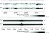 |
Fig. 2 Two examples of spectral segments recorded of η Car plus Weigelt blobs B and D. Top: the spectral region from 2518 to 2560 Å. Bottom: the spectral region from 7000 to 7140 Å. The two segments within each spectral region are from the low state (March 1998) and the ensuing high state (February 1999). Each spectral segment reproduces spatially resolved slit spectra that extends from 0 |
Fewer changes are obvious in the near red between the low and high states (Fig. 2, bottom). Both the central core and the Weigelt blobs exhibit strong high excitation. The He i λ7067 P Cygni and the [Ar iii] λ7137 lines provide examples. During the late low state, diffuse, broad He i emission extends from the central core towards the Weigelt blobs. The [Ar iii] forbidden emission, which defines the wind-wind collision zones, is not present during the low state, but narrow line emission plus complex broad components appear across the high state (Gull et al. 2009; Madura et al. 2012). By the early high state, the broad emission has strengthened, but narrow line emission extends across the Weigelt blobs. We refer to Nielsen et al. (2007a) for discussion on the He i P Cygni profiles that originate deep within the central core in the vicinity of the binary wind-wind interaction structure.
The observations, presented in this atlas, were recorded on March 19, 1998 and February 21, 1999 (HST programs 7302 and 8036) with wavelength coverage from 1640 to 10 400 Å. The spectroscopic low state began in late December, 1997 (JD 2 450 799.8) and extended at least through March, 1998 as demonstrated by low X-ray flux (Corcoran 2005) and confirmed by the lack of high ionization lines of [Ar iii], [Ne iii] and [Fe iii], and weak He i (Damineli et al. 2008a). Full recovery of the X-ray high state was by late summer of 1998, so the February 1999 observations are well into the early stages of the broad spectroscopic high state. Line fluxes of the Weigelt blobs B and D, recorded during a subsequent visit in March 2000, are found to be similar to fluxes in February 1999. From March 1998 to March 2004, a total of six visits were accomplished with the same HST/STIS aperture centered on η Car at the same position angle (or rotated by 180°). Other visits were accomplished at different position angles, of which two (July 2002 and July 2003) were used to observe both η Car and Weigelt D independently, but with the identical position angle for both visits. The importance of the latter two observations is that the July 2, 2002 visit was during the late stages of the broad high state and the July 4, 2003 visit was during the early stages of the several-month-long low state. Line fluxes recorded during the latter visit are quite similar to those of March 1998, the late stage of the previous low state. Since different position angles were used for other observations of η Car, inclusion of Weigelt B and D were not always possible, but spectra of other, similar emission structures, most notably Weigelt C were sometimes within the HST/STIS aperture.
3. The plots and tables
We include the following:
-
Appendix A: summary extracted plots of the February 1999combined spectrum of Weigelt B and D (this spectrum representsthe high state, when all lines are present);
-
Appendix B: spatially-resolved spectro-images recorded during the March 1998 and February 1999 visits with HST/STIS, showing the differences between the low- and high-state spectra (Spectral extractions are also shown with line identifications);
-
Appendix C: list of the identified lines with qualitative relative fluxes and notes calling out additional information.
These data sets will be referenced in following sections that describe the spectral properties and comment on various elements and ionic states. The focus of this paper is on line identification. The wavelength and intensity calibration of STIS has been used, and no additional correction is found necessary for the present analysis.
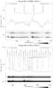 |
Fig. 3 Two examples of spectro-images (spatially-resolved spectra) of η Car, Weigelt B and Weigelt D. Top plot: spectral region from 1892 to 1930 Å recorded during March 1998 and February 1999. The dark streak, labeled “A”, is the spectrum of η Car. Immediately above, labeled “BD”, are the two Weigelt blobs. In the February 1999 (high state) spectrum, a narrow emission of Fe iii 1914.06 Å is prominent, but is absent in the February 1998 spectrum. Much faint continuum extends from the stellar position across the blobs. Velocity shifting absorptions can be seen in both spectra. Absorptions are much more noticeable in the March 1998 (low-state) spectrum. The increase in continuum by Feb. 1999 (high state) is real. Bottom plot: spectral region from 4632 to 4702 Å recorded in the same HST/STIS visits. Narrow emission lines are visible in both spectra with no intervening absorptions. The [Fe iii] 4659.35 Å line is present in the February 1999 (high) spectrum but absent in the March 1998 spectrum. A tilted emission feature at 4662 Å originates from the same line as the red-shifted component from an arcuate-shaped surface associated with the interacting wind cavity (Gull et al. 2009). |
Excerpt of Table C.1.
3.1. Extracted spectra
The high state spectrum recorded in February 1999, extending from 1700 to 10 400 Å, is included in Appendix A to assist the reader in understanding the overall spectral content. Prominent lines and groups of lines are marked. It can be used to find spectral regions relatively devoid of strong nebular lines and to identify areas that are quite confused due to an abundance of nebular emission and/or absorption lines. The spectra also give an overview of the elements present.
3.2. Spectro-images of the spatially resolved structures
Much insight can be obtained by direct examination of the spatially resolved spectra in the form of spectro-images as reproduced in Appendix B. While few absorption lines obscure the BD spectrum in the visible and near-red spectral regions, the ultraviolet spectral region is increasingly dominated by strong absorptions towards shorter wavelengths. Likewise, the nebular line density increases from the red through the visible to the near-ultraviolet around 3000 Å, but then drops as more and more absorption lines overlap the spectrum and as the photon energy associated with the wavelength approaches 8 eV. Indeed, very few nebular lines are identifiable below 2000 Å due both to the increasing absorptions and the dominance of singly-ionized species such as Fe ii and Ni ii.
Two examples of these spectro-images are presented in Fig. 3. In the ultraviolet (Fig. 3, top), the spectra of the Weigelt blobs and of η Car are heavily modulated by absorption lines from singly-ionized species, most notably Fe ii, with ionization potentials below 8 eV and the central source exhibits weak continuum. As mentioned above, the near-diffractive spatial resolution of HST/STIS separates Weigelt B from Weigelt D. By contrast, at wavelengths in the visible (Fig. 3, bottom), line absorptions disappear. η Car is much brighter and contributes significant continuum scatter onto the Weigelt blob positions due both to nebular dust and instrument response. Further into the red, spatial resolution drops even more blending together the spectra of the two Weigelt blobs.
3.3. The line list
The identification of lines in the wavelength region, 1700 to 10 400 Å, results in 2500 identified transitions that are presented in Appendix C. The line list includes the measured and laboratory wavelengths in vacuum, along with line identifications and transition data. To further assist the reader, strong lines have qualitative relative intensities and comments are added for further clarification. In particular, lines produced by fluorescence mechanisms are flagged as well as lines absent in the February 1999 spectrum. The intensities and wavelengths were measured by IDL routines that fitted Gaussian profiles to the observed lines. The intensities are estimated to be accurate to 5–10%, the smaller value for strong lines, but are included for guidance only. Due to blending and intervening absorption, no intensities are given for lines below 2700 Å. The line fluxes are not corrected for interstellar or internal extinction as the properties of extinction from dust located within the Homunculus and the central core are uncertain. Should the reader wish to obtain quantitative flux measures, the on-line spectral data is available through the Hubble Treasury Program2.
A sample of the table is included as Table 1 with notation for abbreviated comments. In the NUV, the line distribution is so dense that blends are very probable, especially with the nebular and instrumental scattered broad stellar line profiles. Multiple possible identifications are given for a number of lines in the NUV. As discussed earlier, the analysis of spectral high-resolution observations by Nielsen et al. (2007b) was used for the region 2424 to 2706 Å.
A number of criteria were used to check the reliability of the line identification for an observed feature. First, consistency checks were made for other lines from the same upper levels, taking the transition probability (A-value) into account. Second, the presence of other lines from the same element at various excitation energies was considered. Third, the excitation distribution for similar elements was considered. In such a complex spectrum, these criteria are more easily fulfilled by iron-group elements, which have numerous possible transitions, compared to simple spectra where only a limited number of lines from a few elements is expected.
4. General appearance of the spectrum
Qualitatively, the line spectrum of the Weigelt blobs range from very crowded in the ultraviolet to sparse in the red, primarily because the density of resonance lines decreases to the red. Absorption dramatically modifies the spectra of the blobs and η Car. External absorption originates from dust and atomic resonance line absorptions from the foreground lobe of the primarily neutral Homunculus ( − 513 km s-1), the internal, ionized Little Homunculus ( − 147 km s-1) and the interstellar medium (0 km s-1) (Nielsen et al. 2005). Intrinsic absorption depresses the flux of η Car relative to the Weigelt blobs (Hillier et al. 2001; Gull et al. 2009) and this effect is greatly accentuated in the blue-visible to the ultraviolet. Moreover, atomic absorption from the foreground Homunculus increasingly dominates the spectrum further into the ultraviolet, where resonance lines of the more-highly excited species might be detected were it not for the dominant intervening absorption.
Few strong, narrow emission lines are seen below 2000 Å, the exceptions being the N iii], Si iii] and C iii] intercombination lines, ⟨ Fe iii ⟩ fluorescence, and some special cases of Fe ii emission discussed in Sect. 6. The 2000 to 2400 Å and 2550 to 2650 Å regions are heavily obscured by intervening broad absorptions from low excitation levels, primarily of Fe ii and Ni ii. The strength and complexity of the absorptions make it increasingly difficult to distinguish between real emission features originating from the Weigelt blobs and merely local regions of lesser absorption. Nebular lines become very dependent upon the characteristically narrow nebular line width and central line velocity. The resonance line absorption towards Weigelt D was investigated by Nielsen et al. (2007b) at resolving power, R = λ/δλ = 100 000, over the wavelength interval 2424 to 2706 Å, thus confirming line identifications listed here and adding two new line identifications for that spectral region. The emission lines observed below 2750 Å are generally rather weak lines from medium-excitation levels of Fe ii and Cr ii, or strong lines of fluorescent Fe ii and [Fe iii].
The 2750 to 3600 Å part of the spectrum is crowded with optically thin lines of low- and medium-excitation iron-group elements, mainly Fe ii. Fluorescent Fe ii produces strong emission around 2850 Å. The 3600 to 4000 Å range is characterized by the Balmer series of hydrogen.
Above 4000 Å, the spectrum is typically nebular in its nature, with strong, narrow emission lines superimposed on a weak, well-defined continuum. The spectrum is dominated by forbidden and low-excitation lines of Fe ii, the other strongest lines coming from H i, He i and [N ii]. A few absorption features are seen, e.g. the Na i doublet at 5890 Å. Some of the emission lines have broad bases of scattered light from the stellar spectrum, as discussed below. All the brightest features above 8000 Å are due to either fluorescent Fe ii or the Paschen series of H i.
4.1. Contributions of extended wind structure
A significant number of narrow and broadened lines seen in the spectro-images do not originate from the Weigelt blobs. They are easily recognized in the 2D spectro-images by an odd tilt angle, compared to the narrow nebular lines being aligned along the direction of the slit, or a broad, diffuse arcuate feature. The obvious clue is that these lines are always in the vicinity of a bright narrow line and are associable with a broad “wind” line in the stellar spectrum. Very bright lines of H i and Fe ii have accompanied diffuse arcs extending from about − 400 to + 400 km s-1 that are visible during both the low and high states. Bright forbidden iron lines show tilted components that come and go. As examples, the [Fe iii] 4659 and 4702 Å lines show a red-shifted arc during the high state that tilts toward lower velocity with distance from η Car. A number of [Fe ii] lines, including 4815 Å, show strong arcuate structure extending in velocity from − 400 to + 400 km s-1 and spatially well above and below the position of η Car during the low state. Analysis of these and other HST/STIS spectra coupled with 3D modeling demonstrated these extended emission structures originate from the ballistic wind-wind interactions of η Car (Gull et al. 2009; Madura et al. 2012). Where these components are noticeable, a note is added for red or blue arc/shell (rd sh, bl sh) in the line list (Appendix C).
5. Representation of the elements
In this section we present discussions about non-iron-group elements producing observed emission lines in the Weigelt spectrum. Since the spectrum is dominated by lines from iron-group elements, especially in the singly-ionized stage, the iron-group elements are discussed separately in Sect. 6.
The two observations discussed below characterize the low and high states in the spectrum of the Weigelt blobs. The March 1998 spectrum is observed during a late phase of the spectroscopic low state, when the high-excitation lines, originating from species with ionization potential is greater that 13.6 eV, are still very weak. The February 1999 spectrum, observed more than a year after low state began, shows the spectrum during the spectroscopic high state. A spectrum recorded in March 2000 by HST/STIS is virtually identical to the February 1999 spectrum. The Weigelt blobs slowly strengthen in high excitation lines throughout the high state which lasts for about five years, then relax rapidly when the low state begins as indicated by ground-based monitoring (Damineli et al. 2008a).
5.1. Hydrogen
The observations cover the entire Balmer series and all but the first three members of the Paschen series. However, the observed spectrum of the Weigelt blobs include nebular-scattered starlight that is heavily dominated by Balmer lines with typical P Cygni profiles: a strong, very broad, spatially-extended emission profile with red-shifted wind and a deep blueshifted absorption. Superimposed on the emission profile is a narrow absorption feature, having a velocity of − 40 to − 50 km s-1 (Johansson et al. 2005). The Paschen lines have simpler line profiles, consisting of a narrow emission peak at − 45 km s-1 superimposed on a broad, asymmetric base of scattered stellar emission. In both series, a narrow emission line at the velocity of the Weigelt blobs is the contribution from the Weigelt blobs. As the apparent brightness of η Car increased with time, the scattered stellar emission peaks increased in intensity in 1999 compared with1998. The nebular components do not appear to increase in brightness.
5.2. Helium
The He i line profiles are greatly influenced by the periodic spectroscopic event. In the 1998 data, only the strongest He i lines, e.g. 2p–3s transitions at 7066 and 7282 Å appear in the Weigelt blob spectrum as broad, asymmetric features, being scattered light from the spectrum of the stellar wind rather than intrinsic radiation from the Weigelt blobs themselves.
In 1999, narrow peaks appear on the broad bases, the observed line profiles being similar to those of the Paschen lines. No narrow He ii lines are observed although broad He ii 4686 Å emission has been observed at the stellar position of η Car during the broad spectroscopic high state, building up to peak strength months before the spectroscopic low state (Damineli et al. 2008a).
5.3. Carbon, oxygen and nitrogen
Like the outer ejecta of η Car (the Little Homunculus, the Homunculus and the fainter nebulosities further outward) the Weigelt blobs appear to have C/N/O abundances characteristic of CNO-cycle hydrogen burning with convection in very massive stars (Meynet & Maeder 2005), i.e. nitrogen is markedly overabundant relative to carbon and oxygen (Verner et al. 2005).
Several N i lines appear throughout the optical and near-IR spectrum, e.g. 3s–3p, 3s–4p, 3p–4d transitions, having excitation energies of ~13 eV. The N i lines are weaker in 1999 than in 1998, whereas the second spectrum of nitrogen is enhanced. The [N ii] λλ5756, 6585, 6549 are among the strongest lines in the optical spectrum in 1999, and the N ii] λλ2139, 2143 appear strong in 1999, being absent in 1998. Also, in 1999 a number of 3s–3p and 3p–3d lines of N ii appear in the optical spectrum. Finally, the N iii] lines at 1750 Å are present in 1999 but not in 1998.
Only one carbon feature is identified in the spectrum. The C iii] intercombination line at 1908 Å is absent in the 1998 data but appears in 1999. Furthermore, there is no evidence that the Fe ii fluorescence pumped by one of the C iv resonance lines at 1548 Å (Johansson 1983), observed in RR Tel (Hartman & Johansson 2000), is working efficiently in the Weigelt blobs, suggesting that the C iv lines are weak, if present at all.
The O i 3s 3S–3p 3P multiplet (opt 4) at 8447 Å, the secondary cascade in the H Lyβ pumping of oxygen proposed by Bowen (1947), is observed in the data. Some of the components of this multiplet may be enhanced by stimulated emission (Johansson & Letokhov 2005; Letokhov & Johansson 2009). The primary fluorescence decay falls at ~1.13 μm, just outside of the observed wavelength range. A feature appearing at 7255.3 Å in the 1999 data, but not present in 1998, is tentatively identified as O i 3p 3P–5s 3S (multiplet 20), but we see no other O i lines from levels of similar excitation energies (e.g. 3p 5P –5s 5S at 6456 Å or 3p 3P–4d 3D at 7004 Å). If the identification of the 7255.3 Å feature is correct, it remains to explain how the upper level of the transition is populated, and why the line is not present in the 1998 data, i.e. close in time to the spectroscopic low state.
The strongest line of the forbidden [O i] multiplet 1F, 3P 2–1D2λ6302, is observed. The 3P1–1D2λ6365 line is blended with [Ni ii]. [O ii] might be present, only weak traces are seen. The 2D–2P lines at 7325 Å and the 4S–2P lines at 2470 Å are blended with other features, and the 4S–2D lines at 3730 Å coincide with the P Cygni profile of H i Balmer 13.
5.4. Neon
Doubly-ionized neon is seen only during the high state. [Ne iii] (isoelectronic to O i) is absent in the 1998 spectrum, but 3P2–1D2 λ3869 is one of the strongest lines in the 3000 to 4000 Å range in 1999. 3P1–1D2λ3968 is also observed in 1999, whereas the transitions from 1S0 are absent. The mechanism behind the variation of these lines during the event was investigated by Johansson & Letokhov (2004b).
5.5. Sodium
The Na i 3s–3p doublet, λλ5891, 5897, appears as a complex absorption feature having multiple velocity components consistent with those catalogued in the NUV spectrum of η Car by Gull et al. (2006). No sodium emission is observed.
5.6. Magnesium
The Mg i intercombination line 3s21S0–3s3p 3P1λ4572 is observed in emission at 4571.72 Å, whereas the 1S0–1P1λ2852 resonance line is observed in absorption. The Mg ii 3s–3p resonance lines λλ2796, 2803 appear as very strong and broad absorption features, having a redshifted emission component. A few other Mg ii lines are observed in emission, e.g. 4s 2S–4p 2P λλ9220, 9246 (multiplet 1), although relatively weak.
5.7. Aluminum
The Al ii intercombination line 3s21S0–3s3p 3P1λ2669 is absent in 1998 but appears in 1999. This is the only convincing evidence of emission lines from any ionization stage of aluminum in the observed spectrum. The Al iii 3s–3p λλ1854, 1862 resonance lines appear as strong absorption features.
5.8. Silicon
In 1999, the Si iii 3s21S0–3s3p 3P1 intercombination line at 1892 Å is the third strongest emission feature in the satellite UV region of the observed spectrum (only the Fe ii λλ2507, 2509 fluorescence lines are stronger). However, there is no sign of the line in the 1998 data. This constitutes one of the most striking examples of the effect of the spectroscopic event on the Weigelt BD spectrum. The excitation of the 1892 Å line has been investigated by Johansson et al. (2006) using the STIS data obtained during the June 2003 event, and is explained by resonance enhanced two-photon ionization (RETPI) from Si ii, leaving Si iii in an excited state.
Si ii is also present in emission. Multiplets 1: (3s3p22D–3s24p 2P) at 3854–3863 Å, 2: (3s24s 2S–3s 24p 2P) at 6348 and 6372 Å, 4: (3s24p 2P–3s25s 2S) at 5958 and 5979 Å, and 5: (3s24p 2S–3s24d 2D) at 5041– 5046 Å are observed both in 1998 and 1999. Multiplet 5 is considerably stronger in 1999 than in 1998. The 3s–3p resonance lines λλ1808, 1816, 1817 are observed in absorption.
5.9. Phosphorus
A line observed at 7876.90 Å is identified as [P ii] 1D2–1S0. This is the strongest transition from the 1S0 level according to calculated transition probabilities (Mendoza & Zeippen 1982). The transitions from 1D2 to the ground term 3P fall outside of the observed wavelength region (~1.2 μm).
5.10. Sulfur
All eight lines belonging to [S ii] multiplets 1F, 2F and 3F (4S–2P, 4S–2D and 2D–2P) are observed in both the low and high state spectra. In the 1999 high state spectrum, [S iii] 3P1,2–1D2 λλ9071, 9533 and 1D2–1S0λ6313 also appear, being relatively strong. 3P1,2–1S0λλ3722, 3798 are blended with H i Balmer lines.
5.11. Chlorine
A line observed at 8579.77 Å is identified as [Cl ii] 3P2–1D2. According to calculations (Mendoza & Zeippen 1983) this is the strongest of the forbidden 3P–1D transitions in Cl ii. The second strongest line, 3P1–1D2λ9126, is blended with an Fe ii fluorescence line. Transitions from the 1S0 level are not observed.
5.12. Argon
[Ar iii] 3P2–1D2λ7137 and 3P1–1D2λ7751 are observed in the February 1999 spectrum. In contrast to the [Ne iii] case, we also observe the two strongest transitions from the 1S0 level, 1D2–1S0λ5193 and 3P1–1S0λ3110. [Ar iii] is not present in the 1998 spectrum. The excitation mechanism was discussed by Johansson & Letokhov (2004b).
5.13. Potassium
The K i 4s–4p resonance lines λλ7667, 7701 are represented by weak, probably interstellar, narrow absorption features. No other potassium lines are observed in the spectrum.
5.14. Calcium
Ca ii emission is represented by multiplets 2 (3d–4p, in the near IR) and 3 (4p–5s, in the near UV). Both lines of the forbidden 4s–3d doublet λλ7293, 7325 are also observed. The H and K resonance lines are strong in absorption at velocities consistent to those catalogued in the NUV by Gull et al. (2006).
5.15. Copper
Two lines of [Cu ii] are observed, 3d10 1S0–3d94s 1D2λ3807 and 3d10 1S0–3d94s 3D2λ4376.
6. The iron-group elements
The entire observed spectrum, from the UV to the near-IR, is characterized by lines from singly-ionized iron-group elements. All elements from titanium to nickel are observed with Fe ii, by the number of lines, being the dominant species.
Scandium is not detected. By contrast, the HST/STIS spectrum of the Strontium Filament, studied by Hartman et al. (2004), includes emission lines of strontium, scandium, vanadium in addition to the iron-peak elements. The Strontium Filament, an ionized metal region, is photo-ionized by radiation with energies less that 7.8 eV. Hence many elements, commonly in doubly-ionized or higher states, survive as neutrals or singly ionized species. The Strontium Filament, with its peculiar metal abundances, has been studied extensively by Bautista et al. (2006, 2009, 2011).
In the following discussion the iron-group lines will be divided into a number of subgroups depending on the energy of the upper levels of the transitions: forbidden lines, low-excitation lines, medium-excitation lines and high-excitation lines. Finally, a description will be given of the appearance of “pseudo-forbidden” lines: lines that are not parity-forbidden, but still come from levels that have relatively long lifetimes and can be regarded as semi-metastable. It is not clear in all cases how these states are populated, but some of them occur in closed loops pumped by H Lyα, e.g. in the same loop as the strong Fe ii 2507, 2509 Å lines. These pseudo-metastable states are of particular interest, since they produce strong emission lines that can be enhanced by stimulated emission (Johansson & Letokhov 2004a).
Higher ionization stages are represented in the 1999 spectrum, but not the 1998 spectrum, by [Fe iii] in particular and by weak lines from [Fe iv] and possibly [Ni iii]. Lines from neutral iron-group elements are absent, with the possible exception of weak Fe i fluorescence, as will be discussed below.
6.1. Forbidden lines
All singly-ionized iron-group elements have many metastable energy levels belonging to the low even-parity configurations 3dk, 3dk−14s and 3dk−24s2. In a low density plasma, such as the Weigelt components, these will give rise to several parity-forbidden emission lines. While forbidden lines in astrophysical plasmas generally are considered to be collisionally excited, many of the metastable states of the iron-group elements are also populated by cascades from odd 4p levels. This makes the use of these lines as diagnostic tools somewhat uncertain (see the discussion on the “pseudo-forbidden” lines below).
The Weigelt blob spectrum is rich in [Fe ii], which dominates the optical region of the spectrum, especially in the 4000 to 6000 Å wavelength range in which the forbidden multiplets 6F (a6D–b4F), 7F (a6D–a6S), 18F (a4F–b4P), 19F (a4F–a4H), 20F (a4F–b4F) and 21F (a4F–a4G) are observed to be very strong. The 14F a4F9/2–a2G9/2λ7157 line is the strongest feature in the spectrum redward of Hα.
Thackeray (1953) reported the presence of blueshifted absorption components of some of the [Fe ii] lines. The velocity associated with the absorption ranged from −395 to −600 km s-1 which he suggested agreed well with that of other strong absorption features in the spectrum, e.g. from H i, Ca ii and Fe ii. While numerous absorption lines of permitted transitions in singly-ionized metals have been observed in high resolution STIS spectra, none were observed in forbidden lines (Gull et al. 2006). One of the dominating components, formed in the Homunculus, has a blueshift of 513 km s-1, but has a characteristic line width of several km s-1. Examination of the twelve [Fe ii] lines listed by Thackeray (1953) shows no absorption features in either the η Car or Weigelt spectra.
Lines of [Ni ii] and [Cr ii] are also present at considerable strengths. The [Ni ii] multiplet 2F (a2D–a2F) at ~7400 Å and the [Cr ii] multiplet 1F (a 6S–a6D) at ~8000 Å produce the strongest emissions. Several lines of [V ii], [Mn ii] and [Co ii] are observed, [Co ii] being the strongest.
Only a few, weak lines are seen of [Ti ii], which on the other hand is prominent in another spatial region of the η Car nebula, the so called Strontium Filament (Hartman et al. 2004). In addition, [Sc ii] is observed in this region but absent in the spectrum of the Weigelt blobs.
6.2. Low-excitation lines
The lowest odd 4p levels of the singly-ionized iron-group elements have excitation energies ranging from ~3.5 eV for Ti ii to ~6.5 eV for Ni ii. The decays from these levels having the highest transition probabilities fall in the 2000–4000 Å wavelength range. Many of the transitions to the lowest lying even parity levels, e.g. the Fe ii multiplets UV1–3 and UV35–36 where the lower levels belong to the ground term a6D and the a4F term 0.3 eV above the ground, are optically thick and show up mostly in absorption. Additional absorptions from intermediate material, as the SE lobe of the Homunculus, result in the strong, broad, blue-shifted absorption profiles that characterize the 2000–3000 Å region of the STIS observations. These absorptions are due mainly to Fe ii, Ni ii and Cr ii. Other transitions are optically thinner, due to higher excitation energies of the lower levels and/or lower transition probabilities, and are observed both in emission and absorption. Examples of such transitions are the UV60–62 Fe ii multiplets and the UV5, UV8 Cr ii multiplets, having emission peaks accompanied by blue-shifted P Cygni profiles.
The z4D and z4F levels in Fe ii can also decay to even 3d64s quartet terms, such as b4P, b4F and a4G, having excitation energies of ~3 eV. These optically thin lines (e.g. multiplets 27, 37, 38, 41, 48, and 49) fall in the optical region of the spectrum, and are observed to be very strong in the Weigelt blobs, the a4G11/2–z4F9/2λ5318 transition being the brightest non-hydrogenic feature in the visible wavelength range. The transition probabilities of these optical lines are smaller than those of the UV lines by 1–2 orders of magnitude, and their strength in the spectrum can be explained by line leakage from the optically thicker line (Jordan 1967; Johansson & Jordan 1984). The optical lines are also observed as strong, broad P Cygni lines in the spectrum of the central star, and their line profiles in the Weigelt spectrum resembles the He i and H i Paschen line profiles, with a narrow peak superimposed on a broad base of scattered star light. The three lines of Fe ii multiplet 42, a6S–z6P, that are observed in many emission line objects are analogous to these lines.
6.3. Medium-excitation lines
Emission from 4p levels in Fe ii and Cr ii having excitation energies between 7.5 and 9.5 eV is observed in the spectrum. The strongest transitions fall in the UV range, between 2400 and 3500 Å. Only a few, weak lines from these levels are seen at longer wavelengths. A possible excitation mechanism for these levels is absorption of continuum radiation below 2000 Å. The UV191 multiplet of Fe ii, a6S–x6P, is also observed. The multiplet consists of three lines having wavelengths of 1785.27, 1786.75 and 1788.00 Å, corresponding to J = 7/2, 5/2 and 3/2 of the x6P term, respectively. The lines are strong in emission in many objects. Various explanations for the population of the upper levels have been given, e.g. photoexcitation by continuum radiation, collisional excitation, and dielectronic recombination (Johansson & Hansen 1988). The λλ1785 and 1786 lines are observed in the Weigelt spectrum, whereas the λ1788 line coincides with an absorption feature due to a Ni ii UV5 line.
Fe ii and Cr ii energy levels that can be populated by absorption of H Lyα ± 5 Å photons.
6.4. High-excitation lines
Absorption of H Lyα photons from the a4D term in Fe ii and the a6D term in Cr ii can populate a number of 4p, 5p, and 4s4p levels having excitation energies between 11 and 12 eV. The primary decays from these levels give rise to strong fluorescence radiation in the UV and near-IR. The secondary decay chain involves lines from the 5s terms e4D and e6D, with excitation energies of ~10 eV, and, in the case of Fe ii, IR lines from the 4s terms c 4P and c4F.
All the Fe ii levels in Table 2, with the possible exceptions of 5p 6F1/2 and 4p 4G7/2 (the transitions from these two levels are blended with other features), produce observed emission lines in the STIS spectrum of the Weigelt components. All of the strongest (non-hydrogenic) emission features between 2000 and 3000 Å, and above 8000 Å are members of the primary and secondary decay chains from these levels. The Cr ii fluorescence lines are considerably weaker than the Fe ii lines due to the lower Cr ii abundance in the Weigelt blobs (Verner et al. 2005). The fluorescence of Cr ii is discussed in more detail by Zethson et al. (2001).
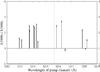 |
Fig. 4 Observed intensity changes of the Fe ii fluorescence lines between 1998 and 1999. Each arrow, placed at the wavelength of the appropriate pumping channel, represents the intensity ratio of I/I of lines originating from one of the pumped levels. Arrows pointing upward indicate an increase; downward a decrease. The dashed vertical line marks the rest wavelength of H Lyα. |
The intensities of the fluorescence lines are, in general, larger in 1999 than in 1998. The magnitude of the intensity changes differs between lines from different upper levels, indicating that the individual pumping channels populating the levels are not equally affected by the spectroscopic event. Figure 4 shows the ratios of the observed intensities of the infrared Fe ii fluorescence lines in the 1999 and 1998 STIS spectra. Included are lines from Fe II levels in Table 3 showing fluorescence lines in the infrared region, except (3P1)4p 4P1/2,3/2 where the fluorescence lines are too blended or weak to derive reliable line ratios. In Fig. 4, each arrow represents lines from one of the levels in Table 2. The horizontal position of an arrow corresponds to the wavelength of the pump channel populating that level. The dashed vertical line marks the rest wavelength of H Lyα. From the figure it is seen that the pumped levels can be divided into three subgroups. The lines from the first group of levels have increased their intensity by a factor of ~2.5 in 1999 as compared to 1998, while the lines from the second group are observed to be stronger by a factor of ~1.5. The upper levels of the λλ2507, 2509 lines, 5p 6F9/2 and 4p 4G9/2, respectively, belong to the first and second group, respectively, and the change in intensity of the two UV lines matches the changes of the IR lines from these two levels. Finally, there is the anomalous case of the lines from 5p 6F3/2 and 5p 6F5/2, whose intensities have decreased in 1999. This strange behavior is hard to explain, especially since the pump channels populating these two levels lie very close in wavelength to transitions populating levels from the first two subgroups.
The Cr ii fluorescence lines are all observed stronger by a factor of 1.5–2 in February 1999 compared with March 1998.
The fluorescence mechanism described above does not explain all the observed Fe ii emission coming from levels with excitation energies larger than 10 eV in the STIS spectrum. Lines from several (5D)5p levels other than those included in Table 2, and also from (4P)4s4p and (4D)4s4p levels, are seen in the near infrared. They are weaker than most of the fluorescence lines, but many of the lines have intensities comparable with lines from other species, e.g. N I. A few lines from Cr ii (5D)5p levels, not included in Table 2, are also observed.
The strongest examples of these lines are the Fe ii multiplets e6D–(5D)5p w6P around 7700 Å, and e6D–(5D)5p 6D around 9300 Å. Photoexcitation of these levels by absorptions of H Lyα photons from the a4D term would require a width of Lyα of more than 30 Å (3700 km s-1), the pump channels having wavelengths of ~1200 Å for the w6P levels and ~1235 Å for the 5p 6D levels. Others of the observed (weaker) lines require even larger widths if they are to be explained as Lyα-induced fluorescence. Such high velocity components of H Lyα are not out of scope as models of the wind-wind interactions leading to the observed X-ray spectra require mass loss velocities of the secondary, η Car B, to be 3000 km s-1 (Pittard & Corcoran 2002). Indeed intensity enhancements of Fe II fluorescent lines are evidence that support greatly broadened wind lines from η Car B.
Another possible excitation mechanism for the lines, resulting from channels with wavelengths more than 5Å from H Lyα, would be photoexcitation from the a6D ground term by continuum radiation, since many of the upper levels in question have strong transition channels at ~1100 Å to a6D levels. A similar process could also explain the presence of several very weak Fe ii lines in the 5000–5500 Å range coming from (5D)4f levels having excitation energies of ~13 eV. These levels are connected to the a4F term with transitions falling at 1000 Å, and their strongest decay channels are to (5D)4d levels, giving rise to the emission lines observed in the STIS spectrum. The (5D)4f levels have J-values of 1/2–15/2, but the J = 13/2 and J = 15/2 levels can not be populated by absorption from the a4F term, the highest J-value of which is 9/2. The proposed excitation mechanism is supported by the fact that no emission lines are seen from the J = 13/2 and J = 15/2 levels, even though the transitions from these levels have the largest transition probabilities of the 4d–4f lines.
The only other examples of emission from highly-excited levels of the iron-group elements are from Mn ii. A number of relatively weak lines between 6123 and 6132 Å are identified as Mn ii 4d e5D–(6S)4f 5F (multiplet 13), the upper levels having excitation energies of ~12 eV. They are seen in emission in other objects as well, e.g. helium-weak stars (Sigut et al. 2000), and have also been observed in earlier observations of η Car. Their appearance in the η Car spectrum has been explained as fluorescence, pumped by the Si ii UV5 multiplet at ~1195 Å (Johansson et al. 1995).
6.5. “Pseudo-forbidden” lines
The following discussion regards Fe ii, but an analogous reasoning is applicable to the other iron-group elements as well.
Figure 5 shows a schematic diagram of the Fe ii term system. The 3d6 configuration in the parent ion, Fe iii, gives rise to 16 different LS terms: 1S, 1S, 1D, 1D, 1F, 1G, 1G, 1I, 3P, 3P, 3D, 3F, 3F, 3G, 3H, and 5D. In accordance with Hund’s rule for equivalent electrons, the 5D term is most tightly bound and is thus the ground term. The two highest terms of the 3d6 configuration, 1S and 1D, have not been found in Fe iii.
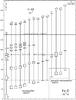 |
Fig. 5 The term system of Fe ii. |
The 3d6 terms of Fe iii are the parent terms of the 3d6nl configurations in Fe ii, and the latter are represented by the boxes in Fig. 5. Each parent term gives rise to a subsystem of Fe ii 3d6(ML)nl configurations, the configurations of the individual subsystems being connected by vertical lines in the figure. The resulting LS- terms of the subconfigurations are obtained by coupling the nl- electron to the ML parent term.
As seen in the figure, the parent structure is closely reproduced by the subconfiguration structure, the distance in energy between the levels of the configurations 3d6(ML)nl and 3d6( )nl in Fe ii being roughly equal to the energy difference between the ML and terms in Fe iii. As a result of this resemblance in structure, the 3d64s configurations belonging to the highest parent terms, b3P, b3F, and b1G are located above the lowest 3d64p levels of the 5D parent, and can consequently decay downwards in allowed 4s → 4p transitions.
These high 4s levels have long lifetimes, being on the order of 1–10 ms, as compared to normal lifetimes of excited levels (1–10 ns). The metastable 3d7 and 3d64s states that give rise to the parity-forbidden emission lines discussed above have lifetimes of 1 ms–10 s, and the high 4s levels can thus be regarded as “pseudo-metastable”. They differ from the metastable states in that they can make allowed transitions down to lower 4p levels. The transition probabilities, or A-values, of these decays are small, having values several orders of magnitude smaller than transitions from normal excited states. But in a low-density plasma producing [Fe ii], such as the Weigelt blobs, they will show up in emission, at wavelengths reaching from the visible (~6000 Å) to the infrared.
A similar case regards the 3d54s2 configuration. (The terms of this configuration can not be assigned to a specific parent term in Fe iii due to the Pauli principle; the 3d54s terms in Fe iii are parent terms of the 3d54snl configurations in Fe ii having nl ≠ 4s.) The 3d54s2 configuration spans a wide energy range, and the highest levels of the configuration lie above the lowest 4p terms, thus producing observable emission lines. The lifetimes of the 3d54s2 levels are shorter than the lifetimes of the high 3d64s levels, ~10 μs. An exception is the lowest level of 3d54s2, a6S5/2, which is metastable and has a lifetime of 0.23 s (Rostohar et al. 2001).
Since the high 3d64s and 3d54s2 levels are of even parity, they can not be pumped from low-lying metastable states by continuum radiation or by a coincidence in wavelength with a strong emission line. Some of the 3d64s levels will be populated by primary cascades of the H Lyα-induced Fe ii fluorescence, but this is an exceptional case in the Weigelt blob spectrum, as no strong emission lines going to the 4s′′ levels are observed. The only strong transitions ending on the 3d54s2 levels come from highly-excited 4s4p and 5p levels above 13 eV, meaning that these levels in general can not be fed by cascades either.
Most of the pseudo-metastable levels are therefore purely collisionally excited, in contrast to many of the true metastable states, which are populated through decays from higher 4p levels. This probably makes the “pseudo-forbidden” emission lines from these levels good diagnostic tools, especially when it comes to abundance studies of the emitting plasma. To our knowledge, these lines have never been used for such purposes.
Many of the pseudo-forbidden Fe ii lines, observed in the Weigelt spectrum, are presented in more detail by Zethson (2001, Appendix A). For further discussions on some of these lines, see Johansson & Zethson (1999) and Johansson et al. (2001). Other examples of similar lines come from Mn ii and Cr ii. The Mn ii 4p z5P–4s 2 c5D multiplet shows up in relatively strong emission between 8000 and 8800 Å. These lines were first identified by Thackeray & Velasco (1976). They are the strongest Mn ii lines in the entire observed spectrum. A number of weak lines above 9500 Å are tentatively identified as Mn ii 4p z5P – 3d6 e3F and 4p z5P–3d6 c3P. This is yet another case of pseudo-forbidden lines, where the highest levels of the 3dk configuration are located above the lowest 3dk−14p levels (cf. Fig. 5), giving rise to 4p–3d transitions. Finally, a few, weak lines are observed from the pseudo-metastable 3d34s2 d4P term in Cr ii.
6.6. Fe i
There is only weak evidence for the presence of neutral iron in Weigelt BD. A feature at 2844.4 Å, partly blended with a stronger Cr ii line, is identified as the a5F2–y5G3λ2844.83 transition in Fe i (UV44). The other lines in the same multiplet coming from the y5G3 level have wavelengths of 2796.36 and 2824.11 Å, respectively. The shorter of these wavelengths almost exactly coincides with the Mg ii 3s–3p resonance line at 2796.35 Å, and since the energy of the a5F-term is low, ~7500 cm-1, the y5G3 level might be pumped by the Mg ii line (Gahm 1974). The 2824.11 Å line, most likely not the line leading to pumping, is unfortunately blended with a Fe ii line (UV198).
No other lines from Fe i or [Fe i] are observed in the spectrum.
6.7. Third spectra lines
[Fe iii] is well represented in the 1999 spectrum, e.g. by multiplets 1F and 3F between 4500 and 5300 Å. A few lines of Fe iii are also observed in the UV; the H Lyα pumped Fe iii fluorescence discussed by Johansson et al. (2000), and also the two strongest lines of the a5S–z5P multiplet (UV 48) at 2070 Å.
A line appearing at 7891 Å in 1999, being absent in 1998, is tentatively identified as the 3F3–1D2 transition of [Ni iii]. The other strong line of that multiplet, 3F2–1D2λ8502 is blended by a Fe ii fluorescence line.
6.8. [Fe iv]
Thirteen rather weak lines, present in the 1999 data but missing in 1998 data, have been identified as [Fe iv]. Some of the proposed [Fe iv] lines are blended with other species, but for a few of the features no other explanations have been found. In a paper on [Fe iv] in RR Tel, Thackeray (1954) notes that a number of unidentified lines in the RR Tel spectrum could be explained as [Fe iv], and that one of these lines also had been observed in η Car, but we have not found any further mentions of [Fe iv] in η Car in the literature. The source of excitation leading to [Fe iv] emission is thought to be the hot companion, η Car B, characterized by Verner et al. (2005); Mehner et al. (2010); Madura et al. (2012) to be an O or WR star capable of ionizing many elements to higher energy states.
The wavelengths, intensities and calculated transition probabilities of the proposed [Fe iv] lines are presented by Zethson (2001, Appendix B).
7. Radial velocities
The radial velocity of the Weigelt blobs can provide clues on when they were ejected from the central star. Previous GHRS observations have shown that the Weigelt blobs have a heliocentric radial velocity of ~−45 km s-1 (Davidson et al. 1997).
Table 3 lists the radial velocities for some of the observed spectral species. The differences among the spectral lines are small, but some discrepancies do exist. Most notably are the velocities of the [N ii] and [Ar iii] lines. [N ii] λ5756 is observed blueshifted by 57 km s-1, while λλ6549, 6585 are blueshifted by 35 and 43 km s-1, respectively. The 5756 Å line originates from the 1S0 level, while the two other lines originate from the 1D2 level. The excitation energy of 1D2 is ~2 eV lower than 1S0, and the difference in observed velocity might suggest that the lines are emitted from different regions in the observed plasma. However, for [Ar iii] the situation is more puzzling. 1S0 → 3P1 λ3110 and 1S0 → 1D2λ5193 have radial velocities of −52 and −59 km s-1, respectively, while 1D2 → 3P2λ7137 and 1D2 → 3P1λ7753 have radial velocities of −41 and −52 km s-1, respectively. Smith et al. (2004) also observe high excitation lines, fluorescent ⟨ Fe ii ⟩ and [Ne iii], to have a larger Doppler shift compared to forbidden [Fe ii] and [Ni ii] lines. A reason for this difference is the possibility that lines are emitted from different parts of the Weigelt condensation as discussed by Hartman et al. (2005). Nielsen et al. (2007b), using the HST/STIS echelle high dispersion mode centered on Weigelt D, measured H i Lyα-pumped lines in the mid-ultraviolet to have heliocentric velocities of −47 ± 0.7 km s-1, in good agreement with the present measures.
Radial velocities for lines from the Weigelt blobs.
All wavelengths in this paper are in vacuum and all velocities are heliocentric.
Acknowledgments
We are grateful to Nick Collins for providing the tools and producing the 2D spectro-images plots. The observations of the Weigelt blobs were made with the STIS on the NASA/ESA HST under programs 7302 and 8036, and were obtained by the Space Telescope Science Institute, which is operated by the Association of Universities for Research in Astronomy, Inc., under NASA contract NAS5-26555. H. Hartman acknowledges support from the Swedish Research Council (VR) through contract 621-2006-3085. The research on η Car at Lund University has received long term support from the Swedish National Space Board (SNSB), which is greatly appreciated. All analysis was done using STIS GTO IDL software tools on data available through the HST η Car Treasury archive. Don Lindler provided very useful display tools for generating the spectro-images. We are grateful to the referee for improvements to the manuscript.
References
- Bautista, M. A., Hartman, H., Gull, T. R., Smith, N., & Lodders, K. 2006, MNRAS, 370, 1991 [NASA ADS] [CrossRef] [Google Scholar]
- Bautista, M. A., Ballance, C., Gull, T. R., et al. 2009, MNRAS, 393, 1503 [NASA ADS] [CrossRef] [Google Scholar]
- Bautista, M. A., Meléndez, M., Hartman, H., Gull, T. R., & Lodders, K. 2011, MNRAS, 410, 2643 [NASA ADS] [CrossRef] [Google Scholar]
- Bowen, I. S. 1947, PASP, 59, 196 [NASA ADS] [CrossRef] [Google Scholar]
- Corcoran, M. F. 2005, AJ, 129, 2018 [NASA ADS] [CrossRef] [Google Scholar]
- Damineli, A. 1996, ApJ, 460, L49 [NASA ADS] [CrossRef] [Google Scholar]
- Damineli, A., Hillier, D. J., Corcoran, M. F., et al. 2008a, MNRAS, 386, 2330 [NASA ADS] [CrossRef] [Google Scholar]
- Damineli, A., Hillier, D. J., Corcoran, M. F., et al. 2008b, MNRAS, 384, 1649 [NASA ADS] [CrossRef] [Google Scholar]
- Davidson, K., Ebbets, D., Weigelt, G., et al. 1995, AJ, 109, 1784 [NASA ADS] [CrossRef] [Google Scholar]
- Davidson, K., Ebbets, D., Johansson, S., Morse, J. A., & Hamann, F. W. 1997, AJ, 113, 335 [NASA ADS] [CrossRef] [Google Scholar]
- Gahm, G. F. 1974, A&AS, 18, 259 [NASA ADS] [Google Scholar]
- Gaviola, E. 1953, ApJ, 118, 234 [NASA ADS] [CrossRef] [Google Scholar]
- Gull, T. R., Ishibashi, K., Davidson, K., & The Cycle 7 STIS GO Team 1999, in Eta Carinae at the Millennium, ed. J. A. Morse, R. M. Humphreys, & A. Damineli, ASP Conf. Ser., 179. 144 [Google Scholar]
- Gull, T. R., Kober, G. V., & Nielsen, K. E. 2006, ApJS, 163, 173 [NASA ADS] [CrossRef] [Google Scholar]
- Gull, T. R., Nielsen, K. E., Corcoran, M. F., et al. 2009, MNRAS, 396, 1308 [NASA ADS] [CrossRef] [Google Scholar]
- Hartman, H., & Johansson, S. 2000, A&A, 359, 627 [NASA ADS] [Google Scholar]
- Hartman, H., Gull, T., Johansson, S., Smith, N., & HST Eta Carinae Treasury Project Team 2004, A&A, 419, 215 [NASA ADS] [CrossRef] [EDP Sciences] [Google Scholar]
- Hartman, H., Damineli, A., Johansson, S., & Letokhov, V. S. 2005, A&A, 436, 945 [NASA ADS] [CrossRef] [EDP Sciences] [Google Scholar]
- Hillier, D. J., Davidson, K., Ishibashi, K., & Gull, T. 2001, ApJ, 553, 837 [NASA ADS] [CrossRef] [Google Scholar]
- Johansson, S. 1983, MNRAS, 205, 71 [NASA ADS] [CrossRef] [Google Scholar]
- Johansson, S., & Hamann, F. 1993, Phys. Scr., T47, 157 [Google Scholar]
- Johansson, S., & Hansen, J. E. 1988, in Physics of Formation of Fe II Lines Outside LTE, ASSL, 138, IAU Colloq., 94, 235 [Google Scholar]
- Johansson, S., & Jordan, C. 1984, MNRAS, 210, 239 [NASA ADS] [Google Scholar]
- Johansson, S., & Letokhov, V. 2001, Science, 291, 625 [NASA ADS] [CrossRef] [Google Scholar]
- Johansson, S., & Letokhov, V. S. 2004a, A&A, 428, 497 [NASA ADS] [CrossRef] [EDP Sciences] [Google Scholar]
- Johansson, S., & Letokhov, V. S. 2004b, Astron. Rep., 48, 399 [NASA ADS] [CrossRef] [Google Scholar]
- Johansson, S., & Letokhov, V. S. 2005, MNRAS, 364, 731 [NASA ADS] [Google Scholar]
- Johansson, S., & Zethson, T. 1999, in ASP Conf. Ser., 179, 171 [Google Scholar]
- Johansson, S., Wallerstein, G., Gilroy, K. K., & Joueizadeh, A. 1995, A&A, 300, 521 [Google Scholar]
- Johansson, S., Zethson, T., Hartman, H., et al. 2000, A&A, 361, 977 [NASA ADS] [Google Scholar]
- Johansson, S., Zethson, T., Hartman, H., & Letokhov, V. 2001, in Eta Carinae and Other Mysterious Stars: The Hidden Opportunities of Emission Line Spectroscopy, ed. T. R. Gull, S. Johansson, & K. Davidson (San Francisco: ASP), ASP Conf. Ser., 242, 297 [Google Scholar]
- Johansson, S., Gull, T. R., Hartman, H., & Letokhov, V. S. 2005, A&A, 435, 183 [NASA ADS] [CrossRef] [EDP Sciences] [Google Scholar]
- Johansson, S., Hartman, H., & Letokhov, V. S. 2006, A&A, 452, 253 [NASA ADS] [CrossRef] [EDP Sciences] [Google Scholar]
- Jordan, C. 1967, Sol. Phys., 2, 441 [NASA ADS] [CrossRef] [Google Scholar]
- Kurucz, R. 2001, http://cfaku5.harvard.edu/atoms.html [Google Scholar]
- Letokhov, V., & Johansson, S. 2009, Astrophysical Lasers (Oxford University Press) [Google Scholar]
- Madura, T. I., Gull, T. R., Owocki, S. P., et al. 2012, MNRAS, 420, 2064 [NASA ADS] [CrossRef] [Google Scholar]
- Mehner, A., Davidson, K., Ferland, G. J., & Humphreys, R. M. 2010, ApJ, 710, 729 [NASA ADS] [CrossRef] [Google Scholar]
- Mendoza, C., & Zeippen, C. J. 1982, MNRAS, 199, 1025 [NASA ADS] [CrossRef] [Google Scholar]
- Mendoza, C., & Zeippen, C. J. 1983, MNRAS, 202, 981 [NASA ADS] [CrossRef] [Google Scholar]
- Meynet, G., & Maeder, A. 2005, A&A, 429, 581 [Google Scholar]
- Neugebauer, G., & Westphal, J. A. 1968, ApJ, 152, L89 [NASA ADS] [CrossRef] [Google Scholar]
- Nielsen, K. E., Gull, T. R., & Vieira Kober, G. 2005, ApJS, 157, 138 [NASA ADS] [CrossRef] [Google Scholar]
- Nielsen, K. E., Corcoran, M. F., Gull, T. R., et al. 2007a, ApJ, 660, 669 [NASA ADS] [CrossRef] [Google Scholar]
- Nielsen, K. E., Ivarsson, S., & Gull, T. R. 2007b, ApJS, 168, 289 [Google Scholar]
- NIST Atomic Spectra Database 2006, http://www.nist.gov/pml/data/asd.cfm [Google Scholar]
- Pittard, J. M., & Corcoran, M. F. 2002, A&A, 383, 636 [NASA ADS] [CrossRef] [EDP Sciences] [Google Scholar]
- Robinson, G., Hyland, A. R., & Thomas, J. A. 1973, MNRAS, 161, 281 [NASA ADS] [Google Scholar]
- Rostohar, D., Derkatch, A., Hartman, H., et al. 2001, Phys. Rev. Lett., 86, 1466 [NASA ADS] [CrossRef] [PubMed] [Google Scholar]
- Sigut, T. A. A., Landstreet, J. D., & Shorlin, S. L. S. 2000, ApJ, 530, L89 [NASA ADS] [CrossRef] [Google Scholar]
- Smith, N., Morse, J. A., Gull, T. R., et al. 2004, ApJ, 605, 405 [NASA ADS] [CrossRef] [Google Scholar]
- Thackeray, A. D. 1953, MNRAS, 113, 211 [NASA ADS] [Google Scholar]
- Thackeray, A. D. 1954, The Observatory, 74, 90 [NASA ADS] [Google Scholar]
- Thackeray, A. D. 1962, MNRAS, 124, 251 [NASA ADS] [Google Scholar]
- Thackeray, A. D. 1967, MNRAS, 135, 51 [NASA ADS] [Google Scholar]
- Thackeray, A. D., & Velasco, R. 1976, The Observatory, 96, 104 [NASA ADS] [Google Scholar]
- Verner, E., Bruhweiler, F., & Gull, T. 2005, ApJ, 624, 973 [NASA ADS] [CrossRef] [Google Scholar]
- Viotti, R., Rossi, L., Cassatella, A., Altamore, A., & Baratta, G. B. 1989, ApJS, 71, 983 [NASA ADS] [CrossRef] [Google Scholar]
- Weigelt, G., & Ebersberger, J. 1986, A&A, 163, L5 [NASA ADS] [Google Scholar]
- Zethson, T. 2001, Ph.D. Thesis, Lund University [Google Scholar]
- Zethson, T., Hartman, H., Johansson, S., et al. 2001, in Eta Carinae and Other Mysterious Stars: The Hidden Opportunities of Emission Spectroscopy, ed. T. R. Gull, S. Johansson, & K. Davidson (San Francisco: ASP), SP Conf. Ser., 242, 97 [Google Scholar]
Appendix A: Overview spectra
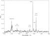 |
Fig. A.1 The 1700–2000 Å spectrum. |
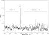 |
Fig. A.2 The 2000–2400 Å spectrum. |
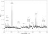 |
Fig. A.3 The 2400–3000 Å spectrum. |
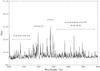 |
Fig. A.4 The 3000–3600 Å spectrum. |
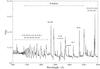 |
Fig. A.5 The 3600–4200 Å spectrum. |
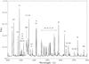 |
Fig. A.6 The 4200–4800 Å spectrum. |
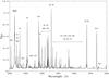 |
Fig. A.7 The 4800–6000 Å spectrum. |
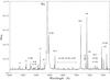 |
Fig. A.8 The 6000–7500 Å spectrum. |
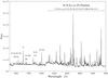 |
Fig. A.9 The 7500–9000 Å spectrum. The dicontinuities seen at 7550 and 8100 Å are not real, but instrumental artifacts caused by overlaps of two adjacent observations. |
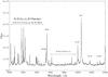 |
Fig. A.10 The 9000–10 400 Å spectrum. For the discontinuity at 9600 Å, see previous figure. |
Appendix B: Spectro-images
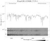 |
Fig. B.1 Spatially-resolved spectra of η Carinae, Weigelt B and Weigelt D. See Fig. 3 and text for detailed information. |
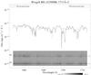 |
Fig. B.2 Spatially-resolved spectra of η Carinae, Weigelt B and Weigelt D. See Fig. 3 and text for detailed information. |
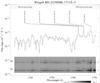 |
Fig. B.3 Spatially-resolved spectra of η Carinae, Weigelt B and Weigelt D. See Fig. 3 and text for detailed information. |
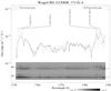 |
Fig. B.4 Spatially-resolved spectra of η Carinae, Weigelt B and Weigelt D. See Fig. 3 and text for detailed information. |
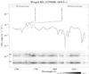 |
Fig. B.5 Spatially-resolved spectra of η Carinae, Weigelt B and Weigelt D. See Fig. 3 and text for detailed information. |
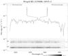 |
Fig. B.6 Spatially-resolved spectra of η Carinae, Weigelt B and Weigelt D. See Fig. 3 and text for detailed information. |
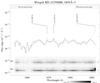 |
Fig. B.7 Spatially-resolved spectra of η Carinae, Weigelt B and Weigelt D. See Fig. 3 and text for detailed information. |
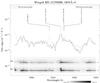 |
Fig. B.8 Spatially-resolved spectra of η Carinae, Weigelt B and Weigelt D. See Fig. 3 and text for detailed information. |
 |
Fig. B.9 Spatially-resolved spectra of η Carinae, Weigelt B and Weigelt D. See Fig. 3 and text for detailed information. |
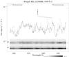 |
Fig. B.10 Spatially-resolved spectra of η Carinae, Weigelt B and Weigelt D. See Fig. 3 and text for detailed information. |
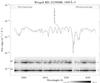 |
Fig. B.11 Spatially-resolved spectra of η Carinae, Weigelt B and Weigelt D. See Fig. 3 and text for detailed information. |
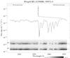 |
Fig. B.12 Spatially-resolved spectra of η Carinae, Weigelt B and Weigelt D. See Fig. 3 and text for detailed information. |
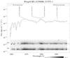 |
Fig. B.13 Spatially-resolved spectra of η Carinae, Weigelt B and Weigelt D. See Fig. 3 and text for detailed information. |
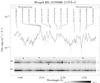 |
Fig. B.14 Spatially-resolved spectra of η Carinae, Weigelt B and Weigelt D. See Fig. 3 and text for detailed information. |
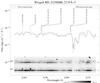 |
Fig. B.15 Spatially-resolved spectra of η Carinae, Weigelt B and Weigelt D. See Fig. 3 and text for detailed information. |
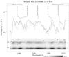 |
Fig. B.16 Spatially-resolved spectra of η Carinae, Weigelt B and Weigelt D. See Fig. 3 and text for detailed information. |
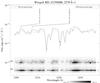 |
Fig. B.17 Spatially-resolved spectra of η Carinae, Weigelt B and Weigelt D. See Fig. 3 and text for detailed information. |
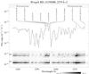 |
Fig. B.18 Spatially-resolved spectra of η Carinae, Weigelt B and Weigelt D. See Fig. 3 and text for detailed information. |
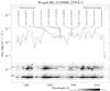 |
Fig. B.19 Spatially-resolved spectra of η Carinae, Weigelt B and Weigelt D. See Fig. 3 and text for detailed information. |
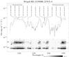 |
Fig. B.20 Spatially-resolved spectra of η Carinae, Weigelt B and Weigelt D. See Fig. 3 and text for detailed information. |
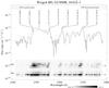 |
Fig. B.21 Spatially-resolved spectra of η Carinae, Weigelt B and Weigelt D. See Fig. 3 and text for detailed information. |
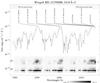 |
Fig. B.22 Spatially-resolved spectra of η Carinae, Weigelt B and Weigelt D. See Fig. 3 and text for detailed information. |
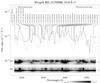 |
Fig. B.23 Spatially-resolved spectra of η Carinae, Weigelt B and Weigelt D. See Fig. 3 and text for detailed information. |
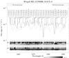 |
Fig. B.24 Spatially-resolved spectra of η Carinae, Weigelt B and Weigelt D. See Fig. 3 and text for detailed information. |
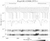 |
Fig. B.25 Spatially-resolved spectra of η Carinae, Weigelt B and Weigelt D. See Fig. 3 and text for detailed information. |
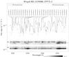 |
Fig. B.26 Spatially-resolved spectra of η Carinae, Weigelt B and Weigelt D. See Fig. 3 and text for detailed information. |
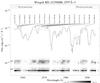 |
Fig. B.27 Spatially-resolved spectra of η Carinae, Weigelt B and Weigelt D. See Fig. 3 and text for detailed information. |
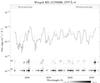 |
Fig. B.28 Spatially-resolved spectra of η Carinae, Weigelt B and Weigelt D. See Fig. 3 and text for detailed information. |
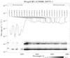 |
Fig. B.29 Spatially-resolved spectra of η Carinae, Weigelt B and Weigelt D. See Fig. 3 and text for detailed information. |
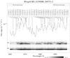 |
Fig. B.30 Spatially-resolved spectra of η Carinae, Weigelt B and Weigelt D. See Fig. 3 and text for detailed information. |
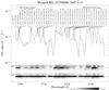 |
Fig. B.31 Spatially-resolved spectra of η Carinae, Weigelt B and Weigelt D. See Fig. 3 and text for detailed information. |
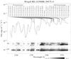 |
Fig. B.32 Spatially-resolved spectra of η Carinae, Weigelt B and Weigelt D. See Fig. 3 and text for detailed information. |
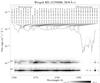 |
Fig. B.33 Spatially-resolved spectra of η Carinae, Weigelt B and Weigelt D. See Fig. 3 and text for detailed information. |
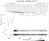 |
Fig. B.34 Spatially-resolved spectra of η Carinae, Weigelt B and Weigelt D. See Fig. 3 and text for detailed information. |
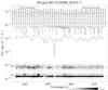 |
Fig. B.35 Spatially-resolved spectra of η Carinae, Weigelt B and Weigelt D. See Fig. 3 and text for detailed information. |
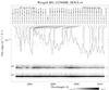 |
Fig. B.36 Spatially-resolved spectra of η Carinae, Weigelt B and Weigelt D. See Fig. 3 and text for detailed information. |
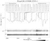 |
Fig. B.37 Spatially-resolved spectra of η Carinae, Weigelt B and Weigelt D. See Fig. 3 and text for detailed information. |
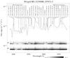 |
Fig. B.38 Spatially-resolved spectra of η Carinae, Weigelt B and Weigelt D. See Fig. 3 and text for detailed information. |
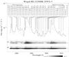 |
Fig. B.39 Spatially-resolved spectra of η Carinae, Weigelt B and Weigelt D. See Fig. 3 and text for detailed information. |
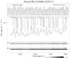 |
Fig. B.40 Spatially-resolved spectra of η Carinae, Weigelt B and Weigelt D. See Fig. 3 and text for detailed information. |
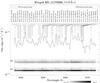 |
Fig. B.41 Spatially-resolved spectra of η Carinae, Weigelt B and Weigelt D. See Fig. 3 and text for detailed information. |
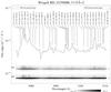 |
Fig. B.42 Spatially-resolved spectra of η Carinae, Weigelt B and Weigelt D. See Fig. 3 and text for detailed information. |
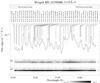 |
Fig. B.43 Spatially-resolved spectra of η Carinae, Weigelt B and Weigelt D. See Fig. 3 and text for detailed information. |
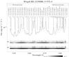 |
Fig. B.44 Spatially-resolved spectra of η Carinae, Weigelt B and Weigelt D. See Fig. 3 and text for detailed information. |
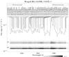 |
Fig. B.45 Spatially-resolved spectra of η Carinae, Weigelt B and Weigelt D. See Fig. 3 and text for detailed information. |
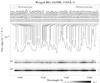 |
Fig. B.46 Spatially-resolved spectra of η Carinae, Weigelt B and Weigelt D. See Fig. 3 and text for detailed information. |
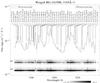 |
Fig. B.47 Spatially-resolved spectra of η Carinae, Weigelt B and Weigelt D. See Fig. 3 and text for detailed information. |
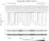 |
Fig. B.48 Spatially-resolved spectra of η Carinae, Weigelt B and Weigelt D. See Fig. 3 and text for detailed information. |
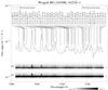 |
Fig. B.49 Spatially-resolved spectra of η Carinae, Weigelt B and Weigelt D. See Fig. 3 and text for detailed information. |
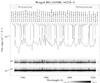 |
Fig. B.50 Spatially-resolved spectra of η Carinae, Weigelt B and Weigelt D. See Fig. 3 and text for detailed information. |
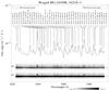 |
Fig. B.51 Spatially-resolved spectra of η Carinae, Weigelt B and Weigelt D. See Fig. 3 and text for detailed information. |
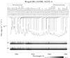 |
Fig. B.52 Spatially-resolved spectra of η Carinae, Weigelt B and Weigelt D. See Fig. 3 and text for detailed information. |
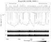 |
Fig. B.53 Spatially-resolved spectra of η Carinae, Weigelt B and Weigelt D. See Fig. 3 and text for detailed information. |
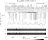 |
Fig. B.54 Spatially-resolved spectra of η Carinae, Weigelt B and Weigelt D. See Fig. 3 and text for detailed information. |
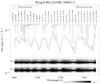 |
Fig. B.55 Spatially-resolved spectra of η Carinae, Weigelt B and Weigelt D. See Fig. 3 and text for detailed information. |
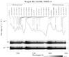 |
Fig. B.56 Spatially-resolved spectra of η Carinae, Weigelt B and Weigelt D. See Fig. 3 and text for detailed information. |
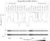 |
Fig. B.57 Spatially-resolved spectra of η Carinae, Weigelt B and Weigelt D. See Fig. 3 and text for detailed information. |
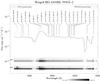 |
Fig. B.58 Spatially-resolved spectra of η Carinae, Weigelt B and Weigelt D. See Fig. 3 and text for detailed information. |
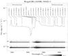 |
Fig. B.59 Spatially-resolved spectra of η Carinae, Weigelt B and Weigelt D. See Fig. 3 and text for detailed information. |
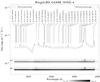 |
Fig. B.60 Spatially-resolved spectra of η Carinae, Weigelt B and Weigelt D. See Fig. 3 and text for detailed information. |
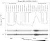 |
Fig. B.61 Spatially-resolved spectra of η Carinae, Weigelt B and Weigelt D. See Fig. 3 and text for detailed information. |
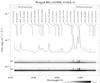 |
Fig. B.62 Spatially-resolved spectra of η Carinae, Weigelt B and Weigelt D. See Fig. 3 and text for detailed information. |
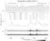 |
Fig. B.63 Spatially-resolved spectra of η Carinae, Weigelt B and Weigelt D. See Fig. 3 and text for detailed information. |
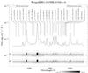 |
Fig. B.64 Spatially-resolved spectra of η Carinae, Weigelt B and Weigelt D. See Fig. 3 and text for detailed information. |
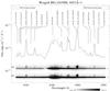 |
Fig. B.65 Spatially-resolved spectra of η Carinae, Weigelt B and Weigelt D. See Fig. 3 and text for detailed information. |
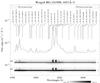 |
Fig. B.66 Spatially-resolved spectra of η Carinae, Weigelt B and Weigelt D. See Fig. 3 and text for detailed information. |
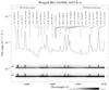 |
Fig. B.67 Spatially-resolved spectra of η Carinae, Weigelt B and Weigelt D. See Fig. 3 and text for detailed information. |
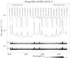 |
Fig. B.68 Spatially-resolved spectra of η Carinae, Weigelt B and Weigelt D. See Fig. 3 and text for detailed information. |
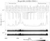 |
Fig. B.69 Spatially-resolved spectra of η Carinae, Weigelt B and Weigelt D. See Fig. 3 and text for detailed information. |
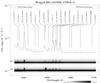 |
Fig. B.70 Spatially-resolved spectra of η Carinae, Weigelt B and Weigelt D. See Fig. 3 and text for detailed information. |
 |
Fig. B.71 Spatially-resolved spectra of η Carinae, Weigelt B and Weigelt D. See Fig. 3 and text for detailed information. |
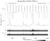 |
Fig. B.72 Spatially-resolved spectra of η Carinae, Weigelt B and Weigelt D. See Fig. 3 and text for detailed information. |
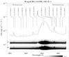 |
Fig. B.73 Spatially-resolved spectra of η Carinae, Weigelt B and Weigelt D. See Fig. 3 and text for detailed information. |
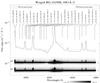 |
Fig. B.74 Spatially-resolved spectra of η Carinae, Weigelt B and Weigelt D. See Fig. 3 and text for detailed information. |
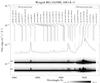 |
Fig. B.75 Spatially-resolved spectra of η Carinae, Weigelt B and Weigelt D. See Fig. 3 and text for detailed information. |
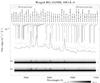 |
Fig. B.76 Spatially-resolved spectra of η Carinae, Weigelt B and Weigelt D. See Fig. 3 and text for detailed information. |
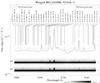 |
Fig. B.77 Spatially-resolved spectra of η Carinae, Weigelt B and Weigelt D. See Fig. 3 and text for detailed information. |
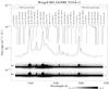 |
Fig. B.78 Spatially-resolved spectra of η Carinae, Weigelt B and Weigelt D. See Fig. 3 and text for detailed information. |
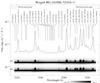 |
Fig. B.79 Spatially-resolved spectra of η Carinae, Weigelt B and Weigelt D. See Fig. 3 and text for detailed information. |
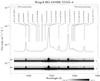 |
Fig. B.80 Spatially-resolved spectra of η Carinae, Weigelt B and Weigelt D. See Fig. 3 and text for detailed information. |
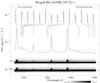 |
Fig. B.81 Spatially-resolved spectra of η Carinae, Weigelt B and Weigelt D. See Fig. 3 and text for detailed information. |
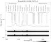 |
Fig. B.82 Spatially-resolved spectra of η Carinae, Weigelt B and Weigelt D. See Fig. 3 and text for detailed information. |
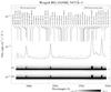 |
Fig. B.83 Spatially-resolved spectra of η Carinae, Weigelt B and Weigelt D. See Fig. 3 and text for detailed information. |
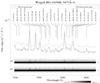 |
Fig. B.84 Spatially-resolved spectra of η Carinae, Weigelt B and Weigelt D. See Fig. 3 and text for detailed information. |
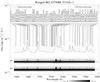 |
Fig. B.85 Spatially-resolved spectra of η Carinae, Weigelt B and Weigelt D. See Fig. 3 and text for detailed information. |
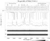 |
Fig. B.86 Spatially-resolved spectra of η Carinae, Weigelt B and Weigelt D. See Fig. 3 and text for detailed information. |
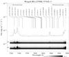 |
Fig. B.87 Spatially-resolved spectra of η Carinae, Weigelt B and Weigelt D. See Fig. 3 and text for detailed information. |
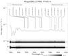 |
Fig. B.88 Spatially-resolved spectra of η Carinae, Weigelt B and Weigelt D. See Fig. 3 and text for detailed information. |
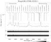 |
Fig. B.89 Spatially-resolved spectra of η Carinae, Weigelt B and Weigelt D. See Fig. 3 and text for detailed information. |
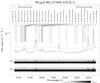 |
Fig. B.90 Spatially-resolved spectra of η Carinae, Weigelt B and Weigelt D. See Fig. 3 and text for detailed information. |
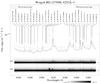 |
Fig. B.91 Spatially-resolved spectra of η Carinae, Weigelt B and Weigelt D. See Fig. 3 and text for detailed information. |
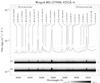 |
Fig. B.92 Spatially-resolved spectra of η Carinae, Weigelt B and Weigelt D. See Fig. 3 and text for detailed information. |
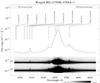 |
Fig. B.93 Spatially-resolved spectra of η Carinae, Weigelt B and Weigelt D. See Fig. 3 and text for detailed information. |
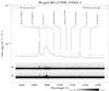 |
Fig. B.94 Spatially-resolved spectra of η Carinae, Weigelt B and Weigelt D. See Fig. 3 and text for detailed information. |
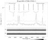 |
Fig. B.95 Spatially-resolved spectra of η Carinae, Weigelt B and Weigelt D. See Fig. 3 and text for detailed information. |
 |
Fig. B.96 Spatially-resolved spectra of η Carinae, Weigelt B and Weigelt D. See Fig. 3 and text for detailed information. |
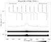 |
Fig. B.97 Spatially-resolved spectra of η Carinae, Weigelt B and Weigelt D. See Fig. 3 and text for detailed information. |
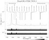 |
Fig. B.98 Spatially-resolved spectra of η Carinae, Weigelt B and Weigelt D. See Fig. 3 and text for detailed information. |
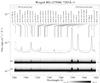 |
Fig. B.99 Spatially-resolved spectra of η Carinae, Weigelt B and Weigelt D. See Fig. 3 and text for detailed information. |
 |
Fig. B.100 Spatially-resolved spectra of η Carinae, Weigelt B and Weigelt D. See Fig. 3 and text for detailed information. |
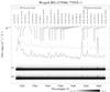 |
Fig. B.101 Spatially-resolved spectra of η Carinae, Weigelt B and Weigelt D. See Fig. 3 and text for detailed information. |
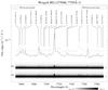 |
Fig. B.102 Spatially-resolved spectra of η Carinae, Weigelt B and Weigelt D. See Fig. 3 and text for detailed information. |
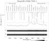 |
Fig. B.103 Spatially-resolved spectra of η Carinae, Weigelt B and Weigelt D. See Fig. 3 and text for detailed information. |
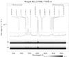 |
Fig. B.104 Spatially-resolved spectra of η Carinae, Weigelt B and Weigelt D. See Fig. 3 and text for detailed information. |
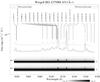 |
Fig. B.105 Spatially-resolved spectra of η Carinae, Weigelt B and Weigelt D. See Fig. 3 and text for detailed information. |
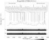 |
Fig. B.106 Spatially-resolved spectra of η Carinae, Weigelt B and Weigelt D. See Fig. 3 and text for detailed information. |
 |
Fig. B.107 Spatially-resolved spectra of η Carinae, Weigelt B and Weigelt D. See Fig. 3 and text for detailed information. |
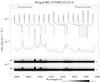 |
Fig. B.108 Spatially-resolved spectra of η Carinae, Weigelt B and Weigelt D. See Fig. 3 and text for detailed information. |
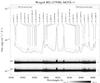 |
Fig. B.109 Spatially-resolved spectra of η Carinae, Weigelt B and Weigelt D. See Fig. 3 and text for detailed information. |
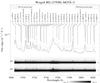 |
Fig. B.110 Spatially-resolved spectra of η Carinae, Weigelt B and Weigelt D. See Fig. 3 and text for detailed information. |
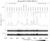 |
Fig. B.111 Spatially-resolved spectra of η Carinae, Weigelt B and Weigelt D. See Fig. 3 and text for detailed information. |
 |
Fig. B.112 Spatially-resolved spectra of η Carinae, Weigelt B and Weigelt D. See Fig. 3 and text for detailed information. |
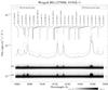 |
Fig. B.113 Spatially-resolved spectra of η Carinae, Weigelt B and Weigelt D. See Fig. 3 and text for detailed information. |
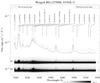 |
Fig. B.114 Spatially-resolved spectra of η Carinae, Weigelt B and Weigelt D. See Fig. 3 and text for detailed information. |
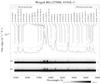 |
Fig. B.115 Spatially-resolved spectra of η Carinae, Weigelt B and Weigelt D. See Fig. 3 and text for detailed information. |
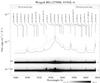 |
Fig. B.116 Spatially-resolved spectra of η Carinae, Weigelt B and Weigelt D. See Fig. 3 and text for detailed information. |
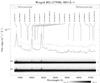 |
Fig. B.117 Spatially-resolved spectra of η Carinae, Weigelt B and Weigelt D. See Fig. 3 and text for detailed information. |
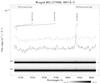 |
Fig. B.118 Spatially-resolved spectra of η Carinae, Weigelt B and Weigelt D. See Fig. 3 and text for detailed information. |
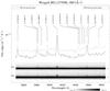 |
Fig. B.119 Spatially-resolved spectra of η Carinae, Weigelt B and Weigelt D. See Fig. 3 and text for detailed information. |
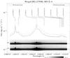 |
Fig. B.120 Spatially-resolved spectra of η Carinae, Weigelt B and Weigelt D. See Fig. 3 and text for detailed information. |
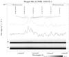 |
Fig. B.121 Spatially-resolved spectra of η Carinae, Weigelt B and Weigelt D. See Fig. 3 and text for detailed information. |
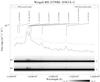 |
Fig. B.122 Spatially-resolved spectra of η Carinae, Weigelt B and Weigelt D. See Fig. 3 and text for detailed information. |
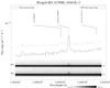 |
Fig. B.123 Spatially-resolved spectra of η Carinae, Weigelt B and Weigelt D. See Fig. 3 and text for detailed information. |
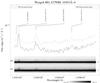 |
Fig. B.124 Spatially-resolved spectra of η Carinae, Weigelt B and Weigelt D. See Fig. 3 and text for detailed information. |
Appendix C: Linelist
Identifications of 2500 emission lines in the wavelength region 1700–10 400 Å from the STIS spectra of the Weigelt blobs recorded in March 1998 and February 1999.
continued.
All Tables
Fe ii and Cr ii energy levels that can be populated by absorption of H Lyα ± 5 Å photons.
Identifications of 2500 emission lines in the wavelength region 1700–10 400 Å from the STIS spectra of the Weigelt blobs recorded in March 1998 and February 1999.
All Figures
|
Fig. 1 Weigelt blobs B and D: taken from an HST/ACS F550M image recorded in 2002, the 2″ × 2″ field of view reveals the complex ejecta surrounding η Car (white core). Three dots define the positions of Weigelt blobs B, C and D. Superimposed (white lines) is the position of the HST/STIS 52″ × 0 |
| In the text | |
|
Fig. 2 Two examples of spectral segments recorded of η Car plus Weigelt blobs B and D. Top: the spectral region from 2518 to 2560 Å. Bottom: the spectral region from 7000 to 7140 Å. The two segments within each spectral region are from the low state (March 1998) and the ensuing high state (February 1999). Each spectral segment reproduces spatially resolved slit spectra that extends from 0 |
| In the text | |
|
Fig. 3 Two examples of spectro-images (spatially-resolved spectra) of η Car, Weigelt B and Weigelt D. Top plot: spectral region from 1892 to 1930 Å recorded during March 1998 and February 1999. The dark streak, labeled “A”, is the spectrum of η Car. Immediately above, labeled “BD”, are the two Weigelt blobs. In the February 1999 (high state) spectrum, a narrow emission of Fe iii 1914.06 Å is prominent, but is absent in the February 1998 spectrum. Much faint continuum extends from the stellar position across the blobs. Velocity shifting absorptions can be seen in both spectra. Absorptions are much more noticeable in the March 1998 (low-state) spectrum. The increase in continuum by Feb. 1999 (high state) is real. Bottom plot: spectral region from 4632 to 4702 Å recorded in the same HST/STIS visits. Narrow emission lines are visible in both spectra with no intervening absorptions. The [Fe iii] 4659.35 Å line is present in the February 1999 (high) spectrum but absent in the March 1998 spectrum. A tilted emission feature at 4662 Å originates from the same line as the red-shifted component from an arcuate-shaped surface associated with the interacting wind cavity (Gull et al. 2009). |
| In the text | |
|
Fig. 4 Observed intensity changes of the Fe ii fluorescence lines between 1998 and 1999. Each arrow, placed at the wavelength of the appropriate pumping channel, represents the intensity ratio of I/I of lines originating from one of the pumped levels. Arrows pointing upward indicate an increase; downward a decrease. The dashed vertical line marks the rest wavelength of H Lyα. |
| In the text | |
|
Fig. 5 The term system of Fe ii. |
| In the text | |
|
Fig. A.1 The 1700–2000 Å spectrum. |
| In the text | |
|
Fig. A.2 The 2000–2400 Å spectrum. |
| In the text | |
|
Fig. A.3 The 2400–3000 Å spectrum. |
| In the text | |
|
Fig. A.4 The 3000–3600 Å spectrum. |
| In the text | |
|
Fig. A.5 The 3600–4200 Å spectrum. |
| In the text | |
|
Fig. A.6 The 4200–4800 Å spectrum. |
| In the text | |
|
Fig. A.7 The 4800–6000 Å spectrum. |
| In the text | |
|
Fig. A.8 The 6000–7500 Å spectrum. |
| In the text | |
|
Fig. A.9 The 7500–9000 Å spectrum. The dicontinuities seen at 7550 and 8100 Å are not real, but instrumental artifacts caused by overlaps of two adjacent observations. |
| In the text | |
|
Fig. A.10 The 9000–10 400 Å spectrum. For the discontinuity at 9600 Å, see previous figure. |
| In the text | |
|
Fig. B.1 Spatially-resolved spectra of η Carinae, Weigelt B and Weigelt D. See Fig. 3 and text for detailed information. |
| In the text | |
|
Fig. B.2 Spatially-resolved spectra of η Carinae, Weigelt B and Weigelt D. See Fig. 3 and text for detailed information. |
| In the text | |
|
Fig. B.3 Spatially-resolved spectra of η Carinae, Weigelt B and Weigelt D. See Fig. 3 and text for detailed information. |
| In the text | |
|
Fig. B.4 Spatially-resolved spectra of η Carinae, Weigelt B and Weigelt D. See Fig. 3 and text for detailed information. |
| In the text | |
|
Fig. B.5 Spatially-resolved spectra of η Carinae, Weigelt B and Weigelt D. See Fig. 3 and text for detailed information. |
| In the text | |
|
Fig. B.6 Spatially-resolved spectra of η Carinae, Weigelt B and Weigelt D. See Fig. 3 and text for detailed information. |
| In the text | |
|
Fig. B.7 Spatially-resolved spectra of η Carinae, Weigelt B and Weigelt D. See Fig. 3 and text for detailed information. |
| In the text | |
|
Fig. B.8 Spatially-resolved spectra of η Carinae, Weigelt B and Weigelt D. See Fig. 3 and text for detailed information. |
| In the text | |
|
Fig. B.9 Spatially-resolved spectra of η Carinae, Weigelt B and Weigelt D. See Fig. 3 and text for detailed information. |
| In the text | |
|
Fig. B.10 Spatially-resolved spectra of η Carinae, Weigelt B and Weigelt D. See Fig. 3 and text for detailed information. |
| In the text | |
|
Fig. B.11 Spatially-resolved spectra of η Carinae, Weigelt B and Weigelt D. See Fig. 3 and text for detailed information. |
| In the text | |
|
Fig. B.12 Spatially-resolved spectra of η Carinae, Weigelt B and Weigelt D. See Fig. 3 and text for detailed information. |
| In the text | |
|
Fig. B.13 Spatially-resolved spectra of η Carinae, Weigelt B and Weigelt D. See Fig. 3 and text for detailed information. |
| In the text | |
|
Fig. B.14 Spatially-resolved spectra of η Carinae, Weigelt B and Weigelt D. See Fig. 3 and text for detailed information. |
| In the text | |
|
Fig. B.15 Spatially-resolved spectra of η Carinae, Weigelt B and Weigelt D. See Fig. 3 and text for detailed information. |
| In the text | |
|
Fig. B.16 Spatially-resolved spectra of η Carinae, Weigelt B and Weigelt D. See Fig. 3 and text for detailed information. |
| In the text | |
|
Fig. B.17 Spatially-resolved spectra of η Carinae, Weigelt B and Weigelt D. See Fig. 3 and text for detailed information. |
| In the text | |
|
Fig. B.18 Spatially-resolved spectra of η Carinae, Weigelt B and Weigelt D. See Fig. 3 and text for detailed information. |
| In the text | |
|
Fig. B.19 Spatially-resolved spectra of η Carinae, Weigelt B and Weigelt D. See Fig. 3 and text for detailed information. |
| In the text | |
|
Fig. B.20 Spatially-resolved spectra of η Carinae, Weigelt B and Weigelt D. See Fig. 3 and text for detailed information. |
| In the text | |
|
Fig. B.21 Spatially-resolved spectra of η Carinae, Weigelt B and Weigelt D. See Fig. 3 and text for detailed information. |
| In the text | |
|
Fig. B.22 Spatially-resolved spectra of η Carinae, Weigelt B and Weigelt D. See Fig. 3 and text for detailed information. |
| In the text | |
|
Fig. B.23 Spatially-resolved spectra of η Carinae, Weigelt B and Weigelt D. See Fig. 3 and text for detailed information. |
| In the text | |
|
Fig. B.24 Spatially-resolved spectra of η Carinae, Weigelt B and Weigelt D. See Fig. 3 and text for detailed information. |
| In the text | |
|
Fig. B.25 Spatially-resolved spectra of η Carinae, Weigelt B and Weigelt D. See Fig. 3 and text for detailed information. |
| In the text | |
|
Fig. B.26 Spatially-resolved spectra of η Carinae, Weigelt B and Weigelt D. See Fig. 3 and text for detailed information. |
| In the text | |
|
Fig. B.27 Spatially-resolved spectra of η Carinae, Weigelt B and Weigelt D. See Fig. 3 and text for detailed information. |
| In the text | |
|
Fig. B.28 Spatially-resolved spectra of η Carinae, Weigelt B and Weigelt D. See Fig. 3 and text for detailed information. |
| In the text | |
|
Fig. B.29 Spatially-resolved spectra of η Carinae, Weigelt B and Weigelt D. See Fig. 3 and text for detailed information. |
| In the text | |
|
Fig. B.30 Spatially-resolved spectra of η Carinae, Weigelt B and Weigelt D. See Fig. 3 and text for detailed information. |
| In the text | |
|
Fig. B.31 Spatially-resolved spectra of η Carinae, Weigelt B and Weigelt D. See Fig. 3 and text for detailed information. |
| In the text | |
|
Fig. B.32 Spatially-resolved spectra of η Carinae, Weigelt B and Weigelt D. See Fig. 3 and text for detailed information. |
| In the text | |
|
Fig. B.33 Spatially-resolved spectra of η Carinae, Weigelt B and Weigelt D. See Fig. 3 and text for detailed information. |
| In the text | |
|
Fig. B.34 Spatially-resolved spectra of η Carinae, Weigelt B and Weigelt D. See Fig. 3 and text for detailed information. |
| In the text | |
|
Fig. B.35 Spatially-resolved spectra of η Carinae, Weigelt B and Weigelt D. See Fig. 3 and text for detailed information. |
| In the text | |
|
Fig. B.36 Spatially-resolved spectra of η Carinae, Weigelt B and Weigelt D. See Fig. 3 and text for detailed information. |
| In the text | |
|
Fig. B.37 Spatially-resolved spectra of η Carinae, Weigelt B and Weigelt D. See Fig. 3 and text for detailed information. |
| In the text | |
|
Fig. B.38 Spatially-resolved spectra of η Carinae, Weigelt B and Weigelt D. See Fig. 3 and text for detailed information. |
| In the text | |
|
Fig. B.39 Spatially-resolved spectra of η Carinae, Weigelt B and Weigelt D. See Fig. 3 and text for detailed information. |
| In the text | |
|
Fig. B.40 Spatially-resolved spectra of η Carinae, Weigelt B and Weigelt D. See Fig. 3 and text for detailed information. |
| In the text | |
|
Fig. B.41 Spatially-resolved spectra of η Carinae, Weigelt B and Weigelt D. See Fig. 3 and text for detailed information. |
| In the text | |
|
Fig. B.42 Spatially-resolved spectra of η Carinae, Weigelt B and Weigelt D. See Fig. 3 and text for detailed information. |
| In the text | |
|
Fig. B.43 Spatially-resolved spectra of η Carinae, Weigelt B and Weigelt D. See Fig. 3 and text for detailed information. |
| In the text | |
|
Fig. B.44 Spatially-resolved spectra of η Carinae, Weigelt B and Weigelt D. See Fig. 3 and text for detailed information. |
| In the text | |
|
Fig. B.45 Spatially-resolved spectra of η Carinae, Weigelt B and Weigelt D. See Fig. 3 and text for detailed information. |
| In the text | |
|
Fig. B.46 Spatially-resolved spectra of η Carinae, Weigelt B and Weigelt D. See Fig. 3 and text for detailed information. |
| In the text | |
|
Fig. B.47 Spatially-resolved spectra of η Carinae, Weigelt B and Weigelt D. See Fig. 3 and text for detailed information. |
| In the text | |
|
Fig. B.48 Spatially-resolved spectra of η Carinae, Weigelt B and Weigelt D. See Fig. 3 and text for detailed information. |
| In the text | |
|
Fig. B.49 Spatially-resolved spectra of η Carinae, Weigelt B and Weigelt D. See Fig. 3 and text for detailed information. |
| In the text | |
|
Fig. B.50 Spatially-resolved spectra of η Carinae, Weigelt B and Weigelt D. See Fig. 3 and text for detailed information. |
| In the text | |
|
Fig. B.51 Spatially-resolved spectra of η Carinae, Weigelt B and Weigelt D. See Fig. 3 and text for detailed information. |
| In the text | |
|
Fig. B.52 Spatially-resolved spectra of η Carinae, Weigelt B and Weigelt D. See Fig. 3 and text for detailed information. |
| In the text | |
|
Fig. B.53 Spatially-resolved spectra of η Carinae, Weigelt B and Weigelt D. See Fig. 3 and text for detailed information. |
| In the text | |
|
Fig. B.54 Spatially-resolved spectra of η Carinae, Weigelt B and Weigelt D. See Fig. 3 and text for detailed information. |
| In the text | |
|
Fig. B.55 Spatially-resolved spectra of η Carinae, Weigelt B and Weigelt D. See Fig. 3 and text for detailed information. |
| In the text | |
|
Fig. B.56 Spatially-resolved spectra of η Carinae, Weigelt B and Weigelt D. See Fig. 3 and text for detailed information. |
| In the text | |
|
Fig. B.57 Spatially-resolved spectra of η Carinae, Weigelt B and Weigelt D. See Fig. 3 and text for detailed information. |
| In the text | |
|
Fig. B.58 Spatially-resolved spectra of η Carinae, Weigelt B and Weigelt D. See Fig. 3 and text for detailed information. |
| In the text | |
|
Fig. B.59 Spatially-resolved spectra of η Carinae, Weigelt B and Weigelt D. See Fig. 3 and text for detailed information. |
| In the text | |
|
Fig. B.60 Spatially-resolved spectra of η Carinae, Weigelt B and Weigelt D. See Fig. 3 and text for detailed information. |
| In the text | |
|
Fig. B.61 Spatially-resolved spectra of η Carinae, Weigelt B and Weigelt D. See Fig. 3 and text for detailed information. |
| In the text | |
|
Fig. B.62 Spatially-resolved spectra of η Carinae, Weigelt B and Weigelt D. See Fig. 3 and text for detailed information. |
| In the text | |
|
Fig. B.63 Spatially-resolved spectra of η Carinae, Weigelt B and Weigelt D. See Fig. 3 and text for detailed information. |
| In the text | |
|
Fig. B.64 Spatially-resolved spectra of η Carinae, Weigelt B and Weigelt D. See Fig. 3 and text for detailed information. |
| In the text | |
|
Fig. B.65 Spatially-resolved spectra of η Carinae, Weigelt B and Weigelt D. See Fig. 3 and text for detailed information. |
| In the text | |
|
Fig. B.66 Spatially-resolved spectra of η Carinae, Weigelt B and Weigelt D. See Fig. 3 and text for detailed information. |
| In the text | |
|
Fig. B.67 Spatially-resolved spectra of η Carinae, Weigelt B and Weigelt D. See Fig. 3 and text for detailed information. |
| In the text | |
|
Fig. B.68 Spatially-resolved spectra of η Carinae, Weigelt B and Weigelt D. See Fig. 3 and text for detailed information. |
| In the text | |
|
Fig. B.69 Spatially-resolved spectra of η Carinae, Weigelt B and Weigelt D. See Fig. 3 and text for detailed information. |
| In the text | |
|
Fig. B.70 Spatially-resolved spectra of η Carinae, Weigelt B and Weigelt D. See Fig. 3 and text for detailed information. |
| In the text | |
|
Fig. B.71 Spatially-resolved spectra of η Carinae, Weigelt B and Weigelt D. See Fig. 3 and text for detailed information. |
| In the text | |
|
Fig. B.72 Spatially-resolved spectra of η Carinae, Weigelt B and Weigelt D. See Fig. 3 and text for detailed information. |
| In the text | |
|
Fig. B.73 Spatially-resolved spectra of η Carinae, Weigelt B and Weigelt D. See Fig. 3 and text for detailed information. |
| In the text | |
|
Fig. B.74 Spatially-resolved spectra of η Carinae, Weigelt B and Weigelt D. See Fig. 3 and text for detailed information. |
| In the text | |
|
Fig. B.75 Spatially-resolved spectra of η Carinae, Weigelt B and Weigelt D. See Fig. 3 and text for detailed information. |
| In the text | |
|
Fig. B.76 Spatially-resolved spectra of η Carinae, Weigelt B and Weigelt D. See Fig. 3 and text for detailed information. |
| In the text | |
|
Fig. B.77 Spatially-resolved spectra of η Carinae, Weigelt B and Weigelt D. See Fig. 3 and text for detailed information. |
| In the text | |
|
Fig. B.78 Spatially-resolved spectra of η Carinae, Weigelt B and Weigelt D. See Fig. 3 and text for detailed information. |
| In the text | |
|
Fig. B.79 Spatially-resolved spectra of η Carinae, Weigelt B and Weigelt D. See Fig. 3 and text for detailed information. |
| In the text | |
|
Fig. B.80 Spatially-resolved spectra of η Carinae, Weigelt B and Weigelt D. See Fig. 3 and text for detailed information. |
| In the text | |
|
Fig. B.81 Spatially-resolved spectra of η Carinae, Weigelt B and Weigelt D. See Fig. 3 and text for detailed information. |
| In the text | |
|
Fig. B.82 Spatially-resolved spectra of η Carinae, Weigelt B and Weigelt D. See Fig. 3 and text for detailed information. |
| In the text | |
|
Fig. B.83 Spatially-resolved spectra of η Carinae, Weigelt B and Weigelt D. See Fig. 3 and text for detailed information. |
| In the text | |
|
Fig. B.84 Spatially-resolved spectra of η Carinae, Weigelt B and Weigelt D. See Fig. 3 and text for detailed information. |
| In the text | |
|
Fig. B.85 Spatially-resolved spectra of η Carinae, Weigelt B and Weigelt D. See Fig. 3 and text for detailed information. |
| In the text | |
|
Fig. B.86 Spatially-resolved spectra of η Carinae, Weigelt B and Weigelt D. See Fig. 3 and text for detailed information. |
| In the text | |
|
Fig. B.87 Spatially-resolved spectra of η Carinae, Weigelt B and Weigelt D. See Fig. 3 and text for detailed information. |
| In the text | |
|
Fig. B.88 Spatially-resolved spectra of η Carinae, Weigelt B and Weigelt D. See Fig. 3 and text for detailed information. |
| In the text | |
|
Fig. B.89 Spatially-resolved spectra of η Carinae, Weigelt B and Weigelt D. See Fig. 3 and text for detailed information. |
| In the text | |
|
Fig. B.90 Spatially-resolved spectra of η Carinae, Weigelt B and Weigelt D. See Fig. 3 and text for detailed information. |
| In the text | |
|
Fig. B.91 Spatially-resolved spectra of η Carinae, Weigelt B and Weigelt D. See Fig. 3 and text for detailed information. |
| In the text | |
|
Fig. B.92 Spatially-resolved spectra of η Carinae, Weigelt B and Weigelt D. See Fig. 3 and text for detailed information. |
| In the text | |
|
Fig. B.93 Spatially-resolved spectra of η Carinae, Weigelt B and Weigelt D. See Fig. 3 and text for detailed information. |
| In the text | |
|
Fig. B.94 Spatially-resolved spectra of η Carinae, Weigelt B and Weigelt D. See Fig. 3 and text for detailed information. |
| In the text | |
|
Fig. B.95 Spatially-resolved spectra of η Carinae, Weigelt B and Weigelt D. See Fig. 3 and text for detailed information. |
| In the text | |
|
Fig. B.96 Spatially-resolved spectra of η Carinae, Weigelt B and Weigelt D. See Fig. 3 and text for detailed information. |
| In the text | |
|
Fig. B.97 Spatially-resolved spectra of η Carinae, Weigelt B and Weigelt D. See Fig. 3 and text for detailed information. |
| In the text | |
|
Fig. B.98 Spatially-resolved spectra of η Carinae, Weigelt B and Weigelt D. See Fig. 3 and text for detailed information. |
| In the text | |
|
Fig. B.99 Spatially-resolved spectra of η Carinae, Weigelt B and Weigelt D. See Fig. 3 and text for detailed information. |
| In the text | |
|
Fig. B.100 Spatially-resolved spectra of η Carinae, Weigelt B and Weigelt D. See Fig. 3 and text for detailed information. |
| In the text | |
|
Fig. B.101 Spatially-resolved spectra of η Carinae, Weigelt B and Weigelt D. See Fig. 3 and text for detailed information. |
| In the text | |
|
Fig. B.102 Spatially-resolved spectra of η Carinae, Weigelt B and Weigelt D. See Fig. 3 and text for detailed information. |
| In the text | |
|
Fig. B.103 Spatially-resolved spectra of η Carinae, Weigelt B and Weigelt D. See Fig. 3 and text for detailed information. |
| In the text | |
|
Fig. B.104 Spatially-resolved spectra of η Carinae, Weigelt B and Weigelt D. See Fig. 3 and text for detailed information. |
| In the text | |
|
Fig. B.105 Spatially-resolved spectra of η Carinae, Weigelt B and Weigelt D. See Fig. 3 and text for detailed information. |
| In the text | |
|
Fig. B.106 Spatially-resolved spectra of η Carinae, Weigelt B and Weigelt D. See Fig. 3 and text for detailed information. |
| In the text | |
|
Fig. B.107 Spatially-resolved spectra of η Carinae, Weigelt B and Weigelt D. See Fig. 3 and text for detailed information. |
| In the text | |
|
Fig. B.108 Spatially-resolved spectra of η Carinae, Weigelt B and Weigelt D. See Fig. 3 and text for detailed information. |
| In the text | |
|
Fig. B.109 Spatially-resolved spectra of η Carinae, Weigelt B and Weigelt D. See Fig. 3 and text for detailed information. |
| In the text | |
|
Fig. B.110 Spatially-resolved spectra of η Carinae, Weigelt B and Weigelt D. See Fig. 3 and text for detailed information. |
| In the text | |
|
Fig. B.111 Spatially-resolved spectra of η Carinae, Weigelt B and Weigelt D. See Fig. 3 and text for detailed information. |
| In the text | |
|
Fig. B.112 Spatially-resolved spectra of η Carinae, Weigelt B and Weigelt D. See Fig. 3 and text for detailed information. |
| In the text | |
|
Fig. B.113 Spatially-resolved spectra of η Carinae, Weigelt B and Weigelt D. See Fig. 3 and text for detailed information. |
| In the text | |
|
Fig. B.114 Spatially-resolved spectra of η Carinae, Weigelt B and Weigelt D. See Fig. 3 and text for detailed information. |
| In the text | |
|
Fig. B.115 Spatially-resolved spectra of η Carinae, Weigelt B and Weigelt D. See Fig. 3 and text for detailed information. |
| In the text | |
|
Fig. B.116 Spatially-resolved spectra of η Carinae, Weigelt B and Weigelt D. See Fig. 3 and text for detailed information. |
| In the text | |
|
Fig. B.117 Spatially-resolved spectra of η Carinae, Weigelt B and Weigelt D. See Fig. 3 and text for detailed information. |
| In the text | |
|
Fig. B.118 Spatially-resolved spectra of η Carinae, Weigelt B and Weigelt D. See Fig. 3 and text for detailed information. |
| In the text | |
|
Fig. B.119 Spatially-resolved spectra of η Carinae, Weigelt B and Weigelt D. See Fig. 3 and text for detailed information. |
| In the text | |
|
Fig. B.120 Spatially-resolved spectra of η Carinae, Weigelt B and Weigelt D. See Fig. 3 and text for detailed information. |
| In the text | |
|
Fig. B.121 Spatially-resolved spectra of η Carinae, Weigelt B and Weigelt D. See Fig. 3 and text for detailed information. |
| In the text | |
|
Fig. B.122 Spatially-resolved spectra of η Carinae, Weigelt B and Weigelt D. See Fig. 3 and text for detailed information. |
| In the text | |
|
Fig. B.123 Spatially-resolved spectra of η Carinae, Weigelt B and Weigelt D. See Fig. 3 and text for detailed information. |
| In the text | |
|
Fig. B.124 Spatially-resolved spectra of η Carinae, Weigelt B and Weigelt D. See Fig. 3 and text for detailed information. |
| In the text | |
Current usage metrics show cumulative count of Article Views (full-text article views including HTML views, PDF and ePub downloads, according to the available data) and Abstracts Views on Vision4Press platform.
Data correspond to usage on the plateform after 2015. The current usage metrics is available 48-96 hours after online publication and is updated daily on week days.
Initial download of the metrics may take a while.