| Issue |
A&A
Volume 539, March 2012
|
|
|---|---|---|
| Article Number | A141 | |
| Number of page(s) | 11 | |
| Section | Astrophysical processes | |
| DOI | https://doi.org/10.1051/0004-6361/201118716 | |
| Published online | 07 March 2012 | |
Kinetic simulation of the electron-cyclotron maser instability: effect of a finite source size
1 Armagh Observatory, Armagh BT61 9DG, Northern Ireland, UK
e-mail: This email address is being protected from spambots. You need JavaScript enabled to view it.
2 Institute of Solar-Terrestrial Physics, 664033 Irkutsk, Russia
3 Irkutsk State Technical University, 664074 Irkutsk, Russia
e-mail: This email address is being protected from spambots. You need JavaScript enabled to view it.
Received: 22 December 2011
Accepted: 30 January 2012
Abstract
Context. The electron-cyclotron maser instability is widespread in the Universe, producing, e.g., radio emission of the magnetized planets and cool substellar objects. Diagnosing the parameters of astrophysical radio sources requires comprehensive nonlinear simulations of the radiation process taking into account the source geometry.
Aims. We simulate the electron-cyclotron maser instability (i.e., the amplification of electromagnetic waves and the relaxation of an unstable electron distribution) in a very low-beta plasma. The model used takes into account the radiation escape from the source region and the particle flow through this region.
Methods. We developed a kinetic code to simulate the time evolution of an electron distribution in a radio emission source. The model includes the terms describing the particle injection to and escape from the emission source region. The spatial escape of the emission from the source is taken into account by using a finite amplification time. The unstable electron distribution of the horseshoe type is considered. A number of simulations were performed for different parameter sets typical of the magnetospheres of planets and ultracool dwarfs.
Results. The generated emission (corresponding to the fundamental extraordinary mode) has a frequency close to the electron cyclotron frequency and propagates across the magnetic field. Shortly after the onset of a simulation, the electron distribution reaches a quasi-stationary state. If the emission source region is relatively small, the resulting electron distribution is similar to that of the injected electrons and the emission intensity is low. In larger sources, the electron distribution may become nearly flat due to the wave-particle interaction, while the conversion efficiency of the particle energy flux into waves reaches 10–20%. We found good agreement of our model with the in situ observations in the source regions of auroral radio emissions of the Earth and Saturn. The expected characteristics of the electron distributions in the magnetospheres of ultracool dwarfs were obtained.
Key words: radiation mechanisms: non-thermal / planets and satellites: aurorae / brown dwarfs / stars: low-mass / radio continuum: stars / radio continuum: planetary systems
© ESO, 2012
1. Introduction
The electron-cyclotron maser instability (ECMI) is believed to be responsible for the generation of auroral radio emissions from the magnetized planets of the solar system (Wu & Lee 1979; Zarka 1998; Treumann 2006). It is very likely that similar radio emissions are also typical of exoplanets (Bastian et al. 2000; Zarka et al. 2001; Zarka 2007; Hess & Zarka 2011), although the sensitivity of the existing instruments does not allow us to detect such radio signals. It was recently discovered that a number of very low-mass stars and brown dwarfs (collectively known as ultracool dwarfs) are the sources of intense periodic radio bursts in the GHz frequency range (Hallinan et al. 2006, 2007, 2008; Berger et al. 2008, 2009); these bursts seem to be produced due to the ECMI in a way similar to the planetary auroral radio emissions, but in a much stronger magnetic field (Kuznetsov et al. 2012). The electron-cyclotron maser has also been suggested as the generation mechanism of the periodic radio bursts from the magnetic Ap star CU Virginis (Trigilio et al. 2000, 2011; Ravi et al. 2010) and of certain types of radio bursts occurring during solar and stellar flares (Melrose & Dulk 1982; Dulk 1985; Fleishman & Melnikov 1998).
The electron-cyclotron maser emission is highly sensitive to the parameters of plasma, magnetic field, and energetic particles in its source. However, utilizing the high diagnostic potential of this emission is a difficult task. Although some parameters of the emission source can be estimated using general features of the maser mechanism (e.g., the emission frequency, as a rule, is very close to the electron cyclotron frequency, which allows us to find the magnetic field strength), most of the source parameters affect the emission properties in a complicated and nonlinear way. A comprehensive nonlinear simulation of the ECMI requires considering the spatial movement of the waves and particles, which requires a lot of computational resources.
In most works devoted to the nonlinear simulation of the ECMI, the spatial movement of waves and particles was simply ignored, which corresponds to an infinite and homogeneous source (the so-called diffusive limit). Kinetic simulations of relaxation of the loss-cone electron distribution in a diffusive limit were performed by Aschwanden & Benz (1988), Aschwanden (1990), and Fleishman & Arzner (2000). Similar simulations for the horseshoe-like distribution are presented in the paper of Kuznetsov (2011,. A number of simulations in a similar approach (i.e., ignoring the source inhomogeneity and finite size) for different electron distributions were performed using the particle-in-cell technique (e.g., Pritchett 1984a,b, 1986b; Pritchett & Strangeway 1985). More complicated particle-in-cell simulations considered an inhomogeneous emission source and used specific boundary conditions and/or numerical methods to account for the radiation escape from the source as well as for the particle flow through the emission source region (Pritchett 1986a; Winglee et al. 1988; Pritchett & Winglee 1989; Pritchett et al. 2002).
In this work, we use a different approach. Like in Paper I, the particles and waves are simulated using a kinetic description. Our model does not explicitly include the spatial movement of the particles and waves and their spatial distributions within the emission source, i.e., the parameters of the particles and waves are treated as averaged over the source volume. The spatial movement of the electromagnetic waves (which results in their escape from the source) is taken into account implicitly by introducing a finite amplification time. In turn, the spatial movement of the electrons is taken into account implicitly by introducing the injection and escape terms in the kinetic equation. Although this model is still oversimplified, we believe it is a much better approximation to reality than the diffusive limit. Like in Paper I, we consider the horseshoe-like distribution of the energetic electrons (e.g., Delory et al. 1998; Ergun et al. 2000; Strangeway et al. 2001). The dispersion relation of the electromagnetic waves is assumed to be similar to that in a vacuum. Simulations are performed for different parameter sets corresponding to the plasma parameters measured in the sources of the auroral radio emissions of the Earth and Saturn, and to the expected parameters of the magnetospheres of ultracool dwarfs. Although our model can in principle be applied to non-stationary processes, we focus here on finding quasi-stationary solutions and analyzing their characteristics.
Generation of terrestrial auroral kilometric radiation in finite-size low-density plasma cavities was studied by Calvert (1981, 1982), Louarn & Le Quéau (1996a,b), Louarn (2006), and Burinskaya & Rauch (2007), who focused on the wave dispersion and propagation and the conditions of radiation escape from the cavity, but did not consider the nonlinear wave-particle interaction. The difference to our work is that, firstly, our aim is to investigate the nonlinear wave-particle interaction, while the wave propagation effects are assumed to be incorporated into a single factor – the wave amplification time. Secondly, we do not consider the possible formation of a discrete spectrum of eigenmodes in a plasma cavity, assuming that the quality factor of such a resonator is too low because of strong energy leakage.
As can be seen from above, we do not consider the formation of fine temporal and spectral structures in the dynamic spectra of radio emission. It was recently proposed that these features may be a reflection of small-scale short-lived nonlinear structures (such as electron holes) in the emission source (e.g., Treumann et al. 2011, 2012). However, simulating the electron-cyclotron maser emission from (or in presence of) electron holes requires a more sophisticated approach and therefore is beyond the scope of this paper.
The numerical model used in the simulations is largely similar to that in Paper I; therefore, most formulae and technical details are omitted and only some important facts and expressions are briefly repeated. We describe our model in Sect. 2. The simulation results (for a wide range of parameters) are presented in Sect. 3. The comparison of the simulation results with the observations is made in Sect. 4. The conclusions are drawn in Sect. 5.
2. Model
2.1. Particle dynamics
Generally, the time evolution of the electron distribution in a stellar/planetary magnetosphere should be described by the Fokker-Planck equation including the effects of the magnetic field convergence, magnetic-field-aligned electric field, and wave-particle interaction (e.g., Hamilton et al. 1990). However, as said above, solving the exact equation would require enormous computational resources because it is necessary to consider explicitly the spatial movement of the particles. In this work, we use a simplified approach where the spatial dependence of the electron distribution function is neglected and the particle movement is treated approximately using the particle fluxes into the considered volume and out of it. Therefore, the kinetic equation for the distribution function f can be written in the form ![Mathematical equation: \begin{equation} \label{fp} \frac{\partial f(\vec{p}, t)}{\partial t}= \left[\frac{\partial f(\vec{p}, t)}{\partial t}\right]_{\mathrm{inj}}+ \left[\frac{\partial f(\vec{p}, t)}{\partial t}\right]_{\mathrm{esc}}+ \left[\frac{\partial f(\vec{p}, t)}{\partial t}\right]_{\mathrm{rel}}, \end{equation}](/articles/aa/full_html/2012/03/aa18716-11/aa18716-11-eq2.png) (1)where p is the electron momentum and the terms (∂f/∂t)inj, (∂f/∂t)esc, and (∂f/∂t)rel describe the injection of the energetic electrons into the considered volume, escape of the electrons from this volume, and variation of the distribution function due to the wave-particle interactions, respectively. The effects of the converging magnetic field and the parallel electric field are assumed to be incorporated into the terms (∂f/∂t)inj and (∂f/∂t)esc, since the escaped electrons can then be reflected from the magnetic mirror and/or re-accelerated by the electric field, so that they re-appear in the simulation model as the injected electrons (but with a different value of the momentum p).
(1)where p is the electron momentum and the terms (∂f/∂t)inj, (∂f/∂t)esc, and (∂f/∂t)rel describe the injection of the energetic electrons into the considered volume, escape of the electrons from this volume, and variation of the distribution function due to the wave-particle interactions, respectively. The effects of the converging magnetic field and the parallel electric field are assumed to be incorporated into the terms (∂f/∂t)inj and (∂f/∂t)esc, since the escaped electrons can then be reflected from the magnetic mirror and/or re-accelerated by the electric field, so that they re-appear in the simulation model as the injected electrons (but with a different value of the momentum p).
We assume that the particle injection is time-independent, so that the corresponding term in Eq. (1) can be written in the form ![Mathematical equation: \begin{equation} \label{df_inj} \left[\frac{\partial f(\vec{p}, t)}{\partial t}\right]_{\mathrm{inj}}= \left(\frac{\partial n_{\mathrm{e}}}{\partial t}\right)_{\mathrm{inj}}\tilde f_{\mathrm{inj}}(\vec{p}), \end{equation}](/articles/aa/full_html/2012/03/aa18716-11/aa18716-11-eq7.png) (2)where (∂ne/∂t)inj is the constant injection rate and
(2)where (∂ne/∂t)inj is the constant injection rate and  is the distribution function of the injected particles, normalized to unity.
The particle escape from the radio emission source can be described by the expression ![Mathematical equation: \begin{equation} \label{df_esc} \left[\frac{\partial f(\vec{p}, t)}{\partial t}\right]_{\mathrm{esc}}= -\frac{f(\vec{p}, t)}{\tau_{\mathrm{esc}}(\vec{p})}, \end{equation}](/articles/aa/full_html/2012/03/aa18716-11/aa18716-11-eq10.png) (3)where τesc is the characteristic escape time. For the particles with constant (time-independent) velocities, the escape time can be estimated as τesc ≃ Rz/|νz|, where Rz is the longitudinal (i.e., along the magnetic field) source size and νz is the longitudinal component of the velocity. However, in situ measurements within the sources of terrestrial and Saturnian auroral radio emissions reveal the presence of magnetic-field-aligned electric fields that accelerate the electrons (Ergun et al. 1998, 2000; Treumann 2006; Lamy et al. 2010; Schippers et al. 2011); as a result, νz ≠ const. and even the particles with zero initial velocity eventually leave the source region. For simplicity, we assume that the particle escape time is constant and is given by the expression
(3)where τesc is the characteristic escape time. For the particles with constant (time-independent) velocities, the escape time can be estimated as τesc ≃ Rz/|νz|, where Rz is the longitudinal (i.e., along the magnetic field) source size and νz is the longitudinal component of the velocity. However, in situ measurements within the sources of terrestrial and Saturnian auroral radio emissions reveal the presence of magnetic-field-aligned electric fields that accelerate the electrons (Ergun et al. 1998, 2000; Treumann 2006; Lamy et al. 2010; Schippers et al. 2011); as a result, νz ≠ const. and even the particles with zero initial velocity eventually leave the source region. For simplicity, we assume that the particle escape time is constant and is given by the expression  (4)where νb is a typical particle speed. In a quasi-stationary state (when the electron density is constant), this model is equivalent to the “recycling” method used in the particle-in-cell simulations by Winglee et al. (1988).
2.2. Wave dynamics
If spatial movement of waves is neglected, the kinetic equation for the waves of mode σ can be written in the form  (5)where
  is the energy density of the waves in the space of wave vectors, k is the wave vector, and γ(σ) is the growth rate (i.e., the above equation describes wave amplification with time due to an instability). The wave-mode index σ is hereafter omitted for brevity.
In Paper I, we considered a diffusive limit in which the wave amplification was limited only by nonlinear effects – relaxation of an unstable electron distribution due to interaction with waves, which resulted in a decrease of the growth rate. In this work, we consider an opposite limit in which the waves are not accumulated in the emission source. Escape of the waves from the amplification region (i.e., from the volume occupied by the electrons with an unstable distribution) naturally limits their intensity. To account for this effect, we assume that (i) the electromagnetic waves are amplified due to the electron-cyclotron maser instability only during a short time interval Δt and (ii) the growth rate remains nearly constant during this time interval. As a result, the maximum energy density of the waves can be estimated as ![Mathematical equation: \begin{equation} \label{Wmax} W_{\vec{k}}^{(\max)}(\vec{k}, t)=W_0(\vec{k})\exp\left[\gamma(\vec{k}, t)\Delta t(\vec{k}, t)\right], \end{equation}](/articles/aa/full_html/2012/03/aa18716-11/aa18716-11-eq24.png) (6)where W0 is some initial energy density (which is determined, e.g., by the spontaneous emission processes).
(6)where W0 is some initial energy density (which is determined, e.g., by the spontaneous emission processes).
The wave amplification time can be estimated as  (7)where Rz, ⊥ are the characteristic sizes of the emission source (along and across the magnetic field, respectively), Δkz, ⊥ are the characteristic sizes of the wave amplification region in the space of wave vectors, and ∂rz, ⊥ /∂t and ∂kz, ⊥ /∂t are the corresponding movement speeds of a wave packet. Escape of the waves from resonance with energetic electrons due to variation of their wave vector in an inhomogeneous medium can be an important factor that affects, e.g., formation of some types of solar radio bursts (Vlasov et al. 2002; Kuznetsov 2006, 2008). However, we consider here the case when the plasma density is very low so that the “vacuum approximation” for the wave dispersion can be used (see below) and the wave vector is nearly independent of the medium parameters and thus on the spatial coordinates; as a result, ∂kz, ⊥ → 0 and the wave escape from resonance in the space of wave vectors is negligible. Also, we consider ring-like or horseshoe-like electron distributions that generate waves mainly in the direction perpendicular to the magnetic field (see, e.g., Paper I). As a result, |∂rz/∂t| ≪ |∂r ⊥ /∂t| and only the spatial escape of the emission from the source in the transverse direction needs to be considered. The expression for the amplification time is then reduced to
  (8)where νgr is the group speed of the waves and θ is their propagation angle relative to the magnetic field. We should note that, according to the satellite measurements, the terrestrial auroral kilometric radiation is generated in auroral cavities that are surrounded by a denser plasma (e.g., Ergun et al. 1998, 2000). The electromagnetic waves can be reflected from the walls of these cavities and return thus increasing the time spent in the emission source. However, the reflected waves will have a different (not perpendicular to the magnetic field) direction of propagation and therefore will not further participate in resonance with the electrons. Therefore the wave amplification time will still be determined by Eq. (8), which now will characterize the time of wave escape from the amplification region in the space of wave vectors.
The formula (6) represents the energy density of the waves that leave the amplification region and thus determines the emission intensity outside the source. By using Eq. (5), we can find the total energy radiated from unit volume per unit time: ![Mathematical equation: \begin{equation} \label{W_rad} \left[\frac{\partial W(t)}{\partial t}\right]_{\mathrm{rad}}= \int\gamma(\vec{k}, t)W_{\vec{k}}^{(\max)}(\vec{k}, t)\,\mathrm{d}^3\vec{k}. \end{equation}](/articles/aa/full_html/2012/03/aa18716-11/aa18716-11-eq36.png) (9)
(9)
2.3. Wave-particle interaction
The variation of the electron distribution due to interaction with the electromagnetic waves is described by the equation (e.g., Aschwanden 1990) ![Mathematical equation: \begin{equation} \label{df_rel} \left[\frac{\partial f(\vec{p}, t)}{\partial t}\right]_{\mathrm{rel}}= \frac{\partial}{\partial p_i}\left[D_{ij}(\vec{p}, t)\frac{\partial f(\vec{p}, t)}{\partial p_j}\right], \end{equation}](/articles/aa/full_html/2012/03/aa18716-11/aa18716-11-eq37.png) (10)where Dij is the diffusion tensor:
(10)where Dij is the diffusion tensor:  (11)ω is the wave frequency and
  is the factor describing the efficiency of the wave-particle interaction (it includes the resonance condition and summation over cyclotron harmonics). If several wave modes can exist simultaneously, then the diffusion tensor Dij is the sum of the tensors (11) for the different modes. In turn, the growth rate of the electromagnetic waves due to interaction with the energetic electrons equals (e.g., Aschwanden 1990)
  (12)The exact expressions for the factor and the methods of calculating the growth rate, diffusion tensor coefficients, and diffusion rate are given in many works (e.g., Melrose & Dulk 1982; Aschwanden & Benz 1988; Aschwanden 1990) and are summarized in Paper I.
When calculating the diffusion tensor (11), we assume that the wave energy density Wk equals its maximum value  given by Eq. (6), since the waves with the highest energy density make the maximum contribution to the relaxation process of an unstable electron distribution. Thus, by using all the assumptions listed in Sects. 2.1–2.3, the time derivative of the electron distribution function ∂f/∂t is reduced to an explicit function of the distribution function itself; in turn, the simulation model is reduced to the differential Eq. (1). In the below simulations, the electron distribution function f(p) is defined on a regular grid in (p,α) space, where α is the electron pitch angle. Equation (1) is numerically integrated with respect to time using the Gear formulae of fourth order with an adaptive stepsize; the details of the numerical code are given in Paper I.
2.4. Model parameters
In situ measurements within the sources of terrestrial and Saturnian auroral radio emissions have revealed that these regions have the following characteristic features (e.g., Treumann 2006; Lamy et al. 2010): (i) the plasma density is very low so that the electron plasma frequency ωp is much lower than the electron cyclotron frequency ωB; (ii) the cold (thermal) electron component is almost absent, so that the energetic electrons with the energy of a few keV dominate. Under these conditions, the dispersion of the electromagnetic waves differs significantly from that in a cold plasma (Pritchett 1984a,b; Le Queau et al. 1984a,b; Winglee 1985; Strangeway 1985, 1986; Robinson 1986, 1987; Le Queau & Louarn 1989; Louarn & Le Quéau 1996b). In particular, numerical simulations by Robinson (1986, 1987) have shown that if the plasma parameters satisfy the condition  (13)the dispersion of the waves (for quasi-transverse propagation) becomes similar to that in a vacuum, i.e., the refraction index N becomes close to unity for both the ordinary and extraordinary waves, the low-frequency cutoff of the X-mode (which is predicted by the cold plasma theory) disappears and the dispersion branches corresponding to the X- and Z-modes of a cold plasma reconnect, forming a single branch (with only a small wiggle near the electron cyclotron frequency). Condition (13) is well satisfied within the sources of terrestrial and Saturnian auroral radio emissions (e.g., Delory et al. 1998; Ergun et al. 2000; Lamy et al. 2010); most likely, radio emissions of other magnetized planets and ultracool dwarfs are produced under similar conditions. In addition, observations of the waves within the sources of terrestrial auroral emission have found no indication of the low-frequency X-mode cutoff (Ergun et al. 1998). Therefore, we adopt here a vacuum-like dispersion relation, with N = 1 and νgr = c for both the ordinary and extraordinary modes. Other details of calculating the growth rate and diffusion tensor for these waves are given in Paper I.
 |
Fig. 1 Quasi-stationary electron distributions for the different values of the particle escape time. Each panel represents a normalized distribution function f/max(f) vs. the normalized momentum p/(mec) and the pitch-angle α. The simulation parameters are given in Sect. 3.1. |
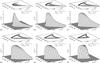 |
Fig. 2 Quasi-stationary growth rates of the extraordinary waves for the different values of the particle escape time. Each panel represents a growth rate γ vs. the normalized frequency ω/ωB and the propagation direction θ. The simulation parameters are given in Sect. 3.1. |
We assume that the injected energetic electrons have a horseshoe-like distribution (Delory et al. 1998; Ergun et al. 2000; Strangeway et al. 2001), which is modeled by the following expression (the same as in Paper I): ![Mathematical equation: \begin{equation} \label{f_inj} \tilde f_{\mathrm{inj}}(\vec{p})=A\exp\left[-\frac{(p-p_{\mathrm{b}})^2}{\Delta p_{\mathrm{b}}^2}\right] \left\{\begin{array}{ll} 1, & \mu\le\mu_{\mathrm{c}},\\ \displaystyle\exp\left[-\frac{(\mu-\mu_{\mathrm{c}})^2}{\Delta\mu_{\mathrm{c}}^2}\right], & \mu>\mu_{\mathrm{c}}, \end{array}\right. \end{equation}](/articles/aa/full_html/2012/03/aa18716-11/aa18716-11-eq59.png) (14)where pb and Δpb are the typical momentum of the injected electrons and their dispersion in momentum, respectively, μ = cosα, μc = cosαc, αc and Δμc are the loss-cone boundary and the boundary width, respectively, and A is the normalization factor. The electrons with 0 ≤ α < π/2 move upward (i.e., toward a decreasing magnetic field), and the electrons with π/2 < α ≤ π move downward (toward an increasing magnetic field). If αc = 0, we obtain an isotropic ring-like distribution.
(14)where pb and Δpb are the typical momentum of the injected electrons and their dispersion in momentum, respectively, μ = cosα, μc = cosαc, αc and Δμc are the loss-cone boundary and the boundary width, respectively, and A is the normalization factor. The electrons with 0 ≤ α < π/2 move upward (i.e., toward a decreasing magnetic field), and the electrons with π/2 < α ≤ π move downward (toward an increasing magnetic field). If αc = 0, we obtain an isotropic ring-like distribution.
The initial wave energy density W0 depends on several factors, including the spontaneous radiation and the emission coming from beyond the considered region. We characterize this energy density by the corresponding effective temperature T0, i.e.  (15)where kB is the Boltzmann constant.
When solving the differential Eq. (1), we are interested in finding a quasi-stationary state with ∂f/∂t → 0. Therefore, the initial electron distribution function (at t = 0) is unimportant. We either assumed that the initial distribution function was equal to zero, or used a result of another simulation as the initial condition for the next simulation run to provide faster convergence. Simulations were stopped when the variation rate of the distribution function fell below a certain threshold (10-3 − 10-2 of the injection rate).
3. Simulation results
3.1. Electron distributions and emission characteristics in a quasi-stationary state
It is easy to show analytically (and is confirmed by our numerical simulations) that for the above described model, the electron distribution with increasing time asymptotically approaches a quasi-stationary state with ∂f/∂t → 0 regardless of the initial distribution, with τesc being the characteristic timescale of this process. The same conclusion can be made for the emission intensity and spectrum, since they are determined by the electron distribution at a given time. Therefore, if the characteristic variation timescales of the observed radio emission far exceed the particle escape time τesc (which implies that the source parameters are stable at those timescales), we can expect that the electron distribution in the emission source has reached a quasi-stationary state or is very close to it. Radio emissions of the planets and ultracool dwarfs, as a rule, satisfy this condition (see Sect. 4). Therefore we focus on the electron distributions and the emission intensities and spectra in a quasi-stationary state.
Firstly, we consider the relative effect of the two factors affecting the electron distribution: particle escape from the radio emission source and relaxation of the electron distribution due to wave-particle interaction. We use the following simulation parameterss (that were chosen to reproduce the observed characteristics of radio emission from ultracool dwarfs, see Sect. 4 for details): the electron cyclotron frequency νB = 4.5 GHz, the transverse size of the emission source R ⊥ = 1000 km, the initial effective temperature of the waves T0 = 106 K, the typical energy of the injected electrons Eb = 10 keV, the relative dispersion of the electrons in momentum Δpb/pb = 0.2, the loss-cone boundary αc = 60°, the loss-cone boundary width Δμc = 0.2, and the electron injection rate (∂ne/∂t)inj = 5 × 106 cm-3 s-1. The particle escape time τesc is variable. Since the extraordinary mode has been found to be strongly dominant under the above conditions (see Sect. 3.2), we consider only this mode in most of our simulations. Figure 1 shows the quasi-stationary electron distributions corresponding to the different values of the particle escape time. Note that the distribution function in each panel of Fig. 1 is normalized to its maximum value, while the actual values of the distribution function increase with τesc, which is indicated by the increasing total electron density ne. Figure 2 shows the corresponding growth rates of the extraordinary waves. Finally, Fig. 3 summarizes the simulation results for the different escape times and shows the maximum growth rate and the total radiation energy flux from unit volume calculated using Eq. (9). The parameter Λ in Figs. 2, 3 is the wave amplification factor that is defined by Λ = Wk/W0; according to Eq. (6), lnΛ = γΔt.
To avoid a possible confusion, we highlight here that Fig. 1 does not represent a temporal evolution of an electron distribution. Instead, each panel in Fig. 1 represents a final (quasi-stationary) stage of such an evolution. These final distributions correspond to different operating conditions of the electron-cyclotron maser, namely, to different longitudinal source sizes Rz, which results in different values of the particle escape time τesc. Accordingly, Fig. 2 represents the final (quasi-stationary) growth rates, while Figs. 3–5 plot some characteristic parameters of the quasi-stationary solutions vs. the emission source parameter τesc.
Figures 1a and 2a correspond to a case when the timescale τesc is very short and thus the particle escape from the emission source region is very fast. In this case, the electron density (and, consequently, the wave growth rate) cannot reach a level sufficient to provide a significant wave amplification. As a result, the relaxation of the electron distribution due to interaction with the waves is negligible and the electron distribution in a quasi-stationary state does not differ from the distribution of the injected electrons . The corresponding electron density equals 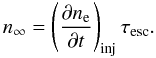 (16)The growth rate has a sharp peak at θ ≃ 90° and ω/ωB ≃ 0.985 that corresponds to the relativistic cyclotron frequency of the electrons with an energy of about 10 keV. The emission intensity is very low (see Fig. 3).
The quasi-stationary growth rate of the waves increases linearly with τesc, until the corresponding wave energy density exceeds a certain threshold so that the wave-particle interaction begins to affect the electron distribution. Under the considered conditions, this happens at lnΛ ≳ 19. Figure 1b shows an example of a weakly relaxed quasi-stationary state at which the electron distribution is only slightly distorted in comparison with the distribution of the injected electrons. In turn, the relaxation of the electron distribution reduces the wave growth rate, so that the growth rate peak broadens and flattens (see Fig. 2b). Note that the wave energy density depends exponentially on the growth rate, and therefore only the waves in a very narrow spectral (Δω/ω ≃ 0.01) and angular (Δθ ≃ 3°) range actually contribute to the total emission intensity as well as to the relaxation of the electron distribution. Although the fraction of the particle energy flux that is transferred to waves is relatively low (about 1% for the state shown in Figs. 1b and 2b), this conversion efficiency can be sufficient to provide, e.g., the observed intensity of terrestrial and Saturnian auroral kilometric radio emissions (Gurnett 1974; Benson & Calvert 1979; Kurth et al. 2005; Lamy et al. 2011).
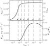 |
Fig. 3 Maximum growth rate (top) and total emission intensity (bottom) of the extraordinary waves in a quasi-stationary state vs. the particle escape time. The vertical lines correspond to the values of τesc shown in Figs. 1, 2. The simulation parameters are given in Sect. 3.1. |
For even higher values of the timescale τesc (Figs. 1c, d), the electrons interact with the waves for a longer time and thus drift farther in velocity space (toward lower velocities) before they eventually leave the radio emission source. As a result, the particle dispersion in velocity increases with τesc; for the case shown in Fig. 1d, the empty space inside the “horseshoe” is almost filled. The maximum growth rate remains nearly constant, but the flattened region around the peak of the growth rate broadens (Figs. 2c, d); therefore, the total emission intensity gradually increases with τesc.
Figures 1e and 2e correspond to the value of the timescale τesc that provides the maximum emission intensity; the conversion efficiency of the particle energy flux into waves in the quasi-stationary state reaches 14.5%. One can see that the empty space around ν = 0 is now completely filled by the electrons; the quasi-stationary electron distribution does not look like a “horseshoe” but rather represents a combination of a nearly flat plateau and a downgoing electron beam (with energy of ~10 keV and the pitch-angle dispersion of ~45°). With a further increase of τesc, the electron distribution does not change qualitatively – the plateau level steadily rises while the beam-like component remains nearly the same (see Fig. 1f). The peak of the wave growth rate becomes narrower (Fig. 2f) and the radio emission characteristics become similar to those for a beam-driven electron-cyclotron instability, i.e., the emission becomes directed slightly downward (with the maximum at θ ≃ 90° − 93°). Although the maximum growth rate slightly increases with τesc, the total emission intensity steadily decreases but remains sufficiently high (with an energy conversion efficiency of ≳ 10%).
Equation (16) for the electron density in a quasi-stationary state n∞ was obtained under the assumption that the wave-particle interaction is negligible. If this interaction is important, the quasi-stationary electron density slightly exceeds n∞ (but by no more than 10-3).
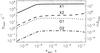 |
Fig. 4 Maximum growth rate of different wave modes in a quasi-stationary state vs. the particle escape time. The simulation parameters are given in Sect. 3.1. |
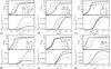 |
Fig. 5 Maximum growth rates and total emission intensities of the extraordinary waves in a quasi-stationary state vs. the particle escape time for the different parameter sets. In each panel, most simulation parameters are the same as in Sect. 3.1, and one parameter (whose values are specified in the panel) is variable. |
Note that the values of the particle escape time used in this section were chosen quite arbitrarily. We have found that different ratios of the particle injection and escape rates together with the wave-particle interaction yield qualitatively different electron distributions and radio emission characteristics. Consequently, the actual characteristics of the particles and radio emission in a planetary or stellar magnetosphere will be determined by the local conditions (such as the emission source dimensions, electron acceleration rate, etc.). In particular, the electron distributions observed in terrestrial or Saturnian magnetosphere seem to be weakly or moderately relaxed like those shown in Figs. 1b, c, while the electron distribution in the magnetospheres of ultracool dwarfs are expected to be strongly relaxed like that shown in Fig. 1f (see Sect. 4 for details).
3.2. Relative contribution of different wave modes
In a low-density plasma (with ωp/ωB ≪ 1), the fundamental extraordinary mode is expected to be the dominant mode of the electron-cyclotron maser (e.g., Wu & Lee 1979; Melrose & Dulk 1982; Sharma & Vlahos 1984; Winglee 1985; Fleishman & Yastrebov 1994; Kuznetsov 2011). This conclusion is generally supported by the observations of the planetary auroral radio emissions (Zarka 1998; Treumann 2006; Ergun et al. 2000; Lamy et al. 2011). To investigate a possible contribution of other wave modes, we performed a simulation considering four modes simultaneously: fundamental and harmonic extraordinary modes (X1 and X2), and fundamental and harmonic ordinary modes (O1 and O2). The simulation parameters were the same as in the previous section.
Figure 4 demonstrates the quasi-stationary growth rates of the considered wave modes corresponding to the different values of the particle escape time τesc. Evidently, the ratios of the growth rates are nearly independent of τesc, i.e., they are nearly the same for both the weakly and strongly relaxed electron distributions. Although the maximum growth rate of the X2-mode somewhat increases at long τesc, it always remains much lower (by more than an order of magnitude) than that of the X1-mode. Since the emission intensity depends exponentially on the growth rate, the X2-mode intensity is lower than that of the X1-mode by a factor of ~109. The growth rates and hence intensities of the O1- and O2-modes are even lower. Therefore we conclude that the X1-mode is strongly dominant under the considered conditions. The intensities of other modes are negligible, and therefore they do not contribute to either the escaping radiation or the relaxation of the electron distribution.
3.3. Effects of varying the model parameters
In Sect. 3.1, we considered the particle and emission characteristics for the different values of the particle escape time from the emission source, i.e., for the different longitudinal sizes of the source. Now we consider the effect of varying the other model parameters. Figure 5 is a collection of plots similar to those in Fig. 3, but corresponding to the different parameter sets. Each panel of Fig. 5 demonstrates the effect of varying a particular model parameter, while the other parameters are assumed to be the same as in Sect. 3.1.
Figure 5a demonstrates the effect of varying the particle injection rate (∂ne/∂t)inj. As expected, an increase of this parameter results in an increase of the emission intensity; the quasi-stationary growth rate of the waves also somewhat increases. In addition, a higher particle injection rate allows the emission to be efficiently produced in smaller sources (i.e., with a shorter particle escape timescale τesc).
Parameters of the considered sources of electron-cyclotron maser radiation.
Figure 5b demonstrates the effect of varying the transverse size of the emission source R ⊥ and hence the wave amplification time Δt. If the particle escape timescale is relatively short, an increase of the transverse source size makes the wave amplification more efficient and thus increases the emission intensity significantly. In contrast, if τesc is long, a larger transverse source size means a stronger relaxation of the electron distribution; this may result in a slight decrease of the emission intensity. Note that we talk here about the average emission energy flux from unit volume (∂W/∂t)rad; the emission intensity from the entire source volume is proportional to  and therefore always increases with R ⊥ . Also note that the actual parameter affecting the wave energy density is the amplification time Δt. If the wave dispersion differs from the “vacuum approximation” used in this work, the amplification time may also be different. However, the effect of increasing or decreasing the wave amplification time will be the same as that shown in Fig. 5b.
Figure 5c demonstrates the effect of varying the initial effective temperature of the waves T0. One can see that this parameter affects the quasi-stationary growth rate of the waves provided that the wave energy density has reached the relaxation threshold (i.e., it is sufficiently high to affect the electron distribution). A higher initial intensity means that the waves need less amplification to reach the mentioned threshold. On the other hand, the emission intensity itself is almost independent of T0. Therefore we conclude that the initial effective temperature of the waves may be chosen quite arbitrarily; in most simulations, we set it to 106 K.
Figure 5d shows the simulation results for the different energies of the injected electrons Eb. Since the particle injection rate (∂ne/∂t)inj is assumed to be constant, an increase of the energy Eb corresponds to an increase of the energy injection rate. In turn, this results in an increase of the emission intensity. The maximum conversion efficiency of the particle energy flux into waves is about 14.5% for all considered values of Eb.
Figure 5e shows the simulation results for the different loss-cone angles of the injected electrons αc. If the injected electrons have the isotropic ring-like distribution (αc = 0), the emission intensity does not exhibit a decrease at high values of τesc; the conversion efficiency of the particle energy flux into waves reaches 12.4%. The highest emission intensity (with the conversion efficiency of up to ~14.5%) is reached for the horseshoe-like distributions with the loss-cone angles of about 60° − 90°. The values of αc > 90° correspond to the beam-like distributions. As the injected electron beam becomes more collimated (i.e., with an increasing αc), the efficiency of the electron-cyclotron maser and hence the emission intensity rapidly decrease; for αc = 120°, the maximum conversion efficiency of the particle energy flux into waves is about 7.0%.
Finally, Fig. 5f demonstrates the effect of varying the dispersion of the injected electrons in momentum Δpb. The nearly monoenergetic electron beams provide a higher growth rate of the waves and possess more free energy than the beams with a higher dispersion in energy. Therefore, a decrease of the parameter Δpb increases the efficiency of the electron-cyclotron maser. One can see in Fig. 5f that in the models with a smaller Δpb, the emission can be efficiently produced in smaller sources, with a shorter particle escape timescale τesc and hence by the electron beams with a lower density. The maximum conversion efficiency of the particle energy flux into waves increases with a decreasing Δpb and reaches 22.4%, 14.5%, and 9.2% for Δpb/pb = 0.1, 0.2, and 0.3, respectively.
Simulation parameters and the resulting radio emission characteristics in a quasi-stationary state for the different radiation sources.
4. Comparison with observations
In this section, we compare the results of our numerical simulations with observations. Namely, we consider the auroral kilometric radio emissions of the Earth and Saturn (for which in situ observations within the source regions are available), and the radio emission of the ultracool dwarf TVLM 513-46546 (hereafter TVLM 513). Table 1 summarizes the main characteristics of these emission sources: the electron cyclotron frequency νB, the L-shell number of the magnetic field line where the source is located, the distance from the planet/star center R (relative to the planet or star radius R0), the spectral intensity of the emission Iobs at the distance d from the source; the transverse size R ⊥ , the electron density ne and energy Eb (where known), and the radiation energy flux per unit volume (∂W/∂t)obs. The latter parameter was estimated in the following way: since the emission frequency ν almost coincides with the local electron cyclotron frequency, the observed emission in the frequency range dν is produced in the volume  , where the height range dz = (dν/ν)LB and LB is the magnetic field inhomogeneity scale along the magnetic field line (for the considered sources, LB ≃ R/3). Therefore, the average radiation energy flux per unit volume can be estimated as
 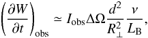 (17)where ΔΩ is the emission solid angle. We used the value of ΔΩ ≃ 0.22 which corresponds to the emission perpendicular to the magnetic field with the beam width of Δθrad ≃ 2°.
Table 2 lists the parameters and results of the simulations. The effective longitudinal source size Rz was calculated as the distance along the magnetic field line between the given point (i.e., where the emission with the given frequency is produced) and the lower (high-frequency) boundary of the radio-emitting region. For the auroral radio emissions of the Earth and Saturn, this boundary corresponds to the electron cyclotron frequency of about 800 kHz (Zarka 1998; Lamy et al. 2011); for TVLM 513, the high-frequency boundary of the radio spectrum is unknown and therefore we assumed that the radio-emitting region extends down to the stellar photosphere (i.e., to R/R0 ≃ 1). The characteristic particle escape time from the emission source region τesc was calculated using Eq. (4), and the loss-cone boundary αc was calculated using the transverse adiabatic invariant: 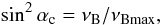 (18)where νBmax is the electron cyclotron frequency at the above-mentioned lower boundary of the radio-emitting region. The electron injection rate was chosen to obtain the specified particle density ne in a quasi-stationary state. In all simulations, we assumed that the initial effective temperature of the electromagnetic waves T0 = 106 K. The simulation results presented include the radiation energy flux from unit volume (∂W/∂t)rad in a quasi-stationary state, the corresponding conversion efficiency of the particle energy flux into waves (∂W/∂t)rad/(∂W/∂t)inj, and the emission beam width (at the 1/e level) Δθrad.
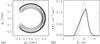 |
Fig. 6 Simulated quasi-stationary electron distribution in the magnetosphere of the Earth (model #1, R⊥ = 100 km). a) 2D distribution function f(pz,p⊥). The pz axis is reversed according to the conventions adopted for the northern hemisphere of the Earth, so that pz < 0 corresponds to the upward direction. b) 1D distribution function in the energy space (integrated over the pitch angle). The dotted line shows the distribution of the injected electrons (i.e., as if the wave-particle interaction were absent). The simulation parameters are given in Table 2. |
Auroral kilometric radiation of the Earth is the best studied among the planetary radio emissions, with a lot of remote and in situ observations (see, e.g., the reviews of Zarka 1998; Treumann 2006). The first model in Table 2 represents a typical source region with the transverse size of ~100 km, average emission intensity (Zarka 1998), and typical electron density and energy (Treumann 2006). The spectrum of the terrestrial radio emission covers a broad frequency range; we chose νB = 400 kHz as a typical example. The simulated electron distribution in a quasi-stationary state1 is shown in Fig. 6. Evidently, the distribution is relatively weakly affected by the wave-particle interaction and does not differ significantly from the distribution of the injected electrons; the surface plot of the distribution function looks similar to that shown in Fig. 1b. The particles are concentrated in a relatively narrow energy range, which agrees with the observations (Treumann 2006). The conversion efficiency of the particle energy flux into waves amounts to only a few percent, but it is sufficient to provide the observed emission intensity (actually, the source size and the electron density and energy may be even lower than in the considered example).
The second model of the source region of the terrestrial auroral radio emission in Table 2 corresponds to a particular event observed by the FAST satellite and reported by Ergun et al. (2000). This event is characterized by an unusually large source size (R⊥ ~ 350 km) and very high emission intensity (far exceeding the average values). We simulated this event using the same parameters as in the previous model, but with an increased transverse source size. As a result, the electron distribution in a quasi-stationary state is now more strongly relaxed (see Fig. 7) and the conversion efficiency of the particle energy flux into waves reaches 11%. Owing to an increased maser efficiency (and larger source volume), the emission intensity is now considerably higher than in the previous model. We have found that by using the observed source dimensions and electron energy and density, we are able to reproduce the observed emission intensity. The calculated electron distribution also looks similar to those observed by FAST (Ergun et al. 2000).
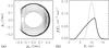 |
Fig. 7 Same as in Fig. 6, for the larger radiation source in the magnetosphere of the Earth (model #2, R ⊥ = 350 km). |
Recently, the Cassini spacecraft crossed the source region of Saturnian kilometric radio emission (Lamy et al. 2010, 2011; Schippers et al. 2011); the basic source parameters measured during this encounter are presented in Table 1. These parameters, however, seem to be quite untypical because, firstly, they correspond to the low-frequency edge of the Saturnian radio emission spectrum (Zarka 1998). The observations were performed at a relatively high altitude; as a result, the loss-cone feature is almost absent (αc ~ 5°) and the particle escape timescale τesc is much longer than that at the Earth. Secondly, the observed emission intensity far exceeds the average values (Zarka 1998). Nevertheless, by using the model based on the observed source dimensions and electron energy and density (see Table 2), we are able to reproduce the observed emission intensity. The simulated quasi-stationary electron distribution (see Fig. 8) agrees with the Cassini observations (Lamy et al. 2010; Mutel et al. 2010). This distribution is slightly more relaxed than that for the second model of the terrestrial auroral radio source; the conversion efficiency of the particle energy flux into waves reaches 13%. We recall, however, that the considered case seems to be fairly uncommon; in a more typical source of Saturnian auroral radio emission, the maser efficiency is expected to be much lower (similar to that at the Earth).
The nearby M9 dwarf TVLM 513 represents a “classic” example of a radio-emitting ultracool dwarf. To date, this object has been detected as a radio source in the 1.4–8.5 GHz frequency range (Jaeger et al. 2011), although the actual spectrum may be broader. In addition to a quiescent component (which may be attributed to the gyrosynchrotron radiation), the radio emission includes short periodic pulses with high brightness temperature and ~100% circular polarization; the pulse period coincides with the stellar rotation period (Hallinan et al. 2006, 2007; Doyle et al. 2010; Kuznetsov et al. 2012). Most likely, the periodic pulses are produced due to the electron-cyclotron maser instability, which requires a magnetic field of ≳3000 G. Kuznetsov et al. (2012) analyzed the radio light curves of TVLM 513 and identified the likely location of the emission source within the stellar magnetosphere (see Table 1) by assuming a dipole magnetic field geometry. We assume that the transverse size of the emission source is similar to that at Saturn (~1000 km), since the radii of the ultracool dwarf and the planet are comparable. We also assume that the typical electron energy in the magnetosphere of the ultracool dwarf is similar to that at the Earth and Saturn (~10 keV), although it may actually be higher, as suggested by the presence of a considerable gyrosynchrotron component in the radio emission. The electron injection rate (∂ne/∂t)inj = 5 × 106 cm-3 s-1 was chosen to provide the observed emission intensity. The resulting electron density in a quasi-stationary state is ne ≃ 4.2 × 105 cm-3. This is much higher than in the planetary magnetospheres, but the corresponding plasma-to-cyclotron frequency ratio (ωp/ωB ≃ 10-3) is even lower than in the sources of auroral radio emissions of the Earth and Saturn, and is comparable with the estimations for Jupiter (Lecacheux et al. 1991; Melrose & Dulk 1991). The simulated quasi-stationary electron distribution (see Figs. 1f and 9) is strongly relaxed and nearly flat. Therefore we expect the electron distributions in the magnetospheres of ultracool dwarfs to differ significantly from the shell- or horseshoe-like distributions that are typical of the source regions of planetary auroral radio emissions. Instead, we expect them to look similar to Maxwellian or kappa distributions, which are only slightly distorted by the parallel electric field and magnetic mirroring (i.e., the particle scattering on the waves is strong enough to keep the electron distribution close to an equilibrium state). Nevertheless, even these small deviations from an equilibrium distribution seem to be sufficient to produce an intense radio emission.
The typical duration of radio pulses from TVLM 513 is about tens of seconds; moreover, the individual pulses seem to be caused by the star’s rotation when a narrow radio beam sweeps periodically over an observer (Hallinan et al. 2006, 2007, 2008; Berger et al. 2009; Kuznetsov et al. 2012), while the parameters of the emission source region are stable at the timescales comparable to or exceeding the rotation period (≃2 h). These timescales far exceed the estimated timescale of the particle escape from the emission source (τesc ~ 0.084 s). Therefore the assumption that the electron distribution has reached a quasi-stationary state is well justified.
5. Conclusion
We have performed numerical simulations of the electron-cyclotron maser instability in a very low-density plasma. Our kinetic model included the relaxation of the electron distribution due to the wave-particle interaction, the injection of the energetic electrons with an unstable distribution into the emission source region, and the escape of the electrons from that region. A finite amplification time of the electromagnetic waves (caused by their escape from the source) was taken into account. The injected electrons were assumed to have the horseshoe-like distribution. We have found that
-
The produced radio emission corresponds to the fundamentalextraordinary mode, with a frequency slightly below the electroncyclotron frequency and the propagation direction nearlyperpendicular to the magnetic field. This conclusion is valid bothfor the cases when the electron distribution is similar to that of theinjected electrons, and when it is strongly relaxed. The intensityof other wave modes is negligible. In a relatively short time (whichis determined by the particle escape time from the emissionsource region), the electron distribution and hence the emissionintensity and spectrum reach a quasi-stationary state.
-
Under conditions typical of the sources of terrestrial and Saturnian auroral radio emissions, the dominant factor affecting the electron distribution is the particle escape from the emission source region. As a result, the electron distribution in a quasi-stationary state is weakly relaxed, i.e., it does not differ significantly from the horseshoe-like distribution of the injected electrons. The conversion efficiency of the particle energy flux into waves is typically a few percent, although it may be higher in particular events. The emission escape from the source region has a “stabilizing” effect on the electron distribution, i.e., it reduces the maser efficiency and allows the particles to have highly nonequilibrium but long-living (quasi-stationary) distributions. The simulated emission intensities and electron distributions agree well with the observations.
-
Radio emission from ultracool dwarfs is much more intense than the planetary radio emissions. Therefore we expect that in the magnetospheres of ultracool dwarfs, the dominant factor affecting the electron distribution is the wave-particle interaction. As a result, the electron distribution in a quasi-stationary state is strongly relaxed and nearly flat; the conversion efficiency of the particle energy flux into waves is about 10%. The radiation directivity pattern slightly differs from that for a shell- or horseshoe-driven instability; in particular, the emission is directed slightly downward. The energetic electrons with a relatively low density (ωp/ωB ~ 10-3) and energy of ~10 keV are able to provide the observed emission intensity.
Acknowledgments
A. A. Kuznetsov thanks the Leverhulme Trust for financial support. Research at Armagh Observatory is grant-aided by the Northern Ireland Department of Culture, Arts and Leisure.
References
- Aschwanden, M. J. 1990, A&AS, 85, 1141 [NASA ADS] [Google Scholar]
- Aschwanden, M. J., & Benz, A. O. 1988, ApJ, 332, 447 [NASA ADS] [CrossRef] [Google Scholar]
- Bastian, T. S., Dulk, G. A., & Leblanc, Y. 2000, ApJ, 545, 1058 [NASA ADS] [CrossRef] [Google Scholar]
- Benson, R. F., & Calvert, W. 1979, Geophys. Res. Lett., 6, 479 [NASA ADS] [CrossRef] [Google Scholar]
- Berger, E., Gizis, J. E., Giampapa, M. S., et al. 2008, ApJ, 673, 1080 [NASA ADS] [CrossRef] [Google Scholar]
- Berger, E., Rutledge, R. E., Phan-Bao, N., et al. 2009, ApJ, 695, 310 [NASA ADS] [CrossRef] [Google Scholar]
- Burinskaya, T. M., & Rauch, J. L. 2007, Plasma Phys. Rep., 33, 28 [NASA ADS] [CrossRef] [Google Scholar]
- Calvert, W. 1981, Geophys. Res. Lett., 8, 919 [NASA ADS] [CrossRef] [Google Scholar]
- Calvert, W. 1982, J. Geophys. Res., 87, 8199 [NASA ADS] [CrossRef] [Google Scholar]
- Delory, G. T., Ergun, R. E., Carlson, C. W., et al. 1998, Geophys. Res. Lett., 25, 2069 [Google Scholar]
- Doyle, J. G., Antonova, A., Marsh, M. S., et al. 2010, A&A, 524, A15 [NASA ADS] [CrossRef] [EDP Sciences] [Google Scholar]
- Dulk, G. A. 1985, ARA&A, 23, 169 [NASA ADS] [CrossRef] [Google Scholar]
- Ergun, R. E., Carlson, C. W., McFadden, J. P., et al. 1998, Geophys. Res. Lett., 25, 2061 [NASA ADS] [CrossRef] [Google Scholar]
- Ergun, R. E., Carlson, C. W., McFadden, J. P., et al. 2000, ApJ, 538, 456 [NASA ADS] [CrossRef] [Google Scholar]
- Fleishman, G., & Arzner, K. 2000, A&A, 358, 776 [NASA ADS] [Google Scholar]
- Fleishman, G. D., & Melnikov, V. F. 1998, Soviet Physics Uspekhi, 41, 1157 [NASA ADS] [CrossRef] [Google Scholar]
- Fleishman, G. D., & Yastrebov, S. G. 1994, Sol. Phys., 153, 389 [NASA ADS] [CrossRef] [Google Scholar]
- Gurnett, D. A. 1974, J. Geophys. Res., 79, 4227 [NASA ADS] [CrossRef] [Google Scholar]
- Hallinan, G., Antonova, A., Doyle, J. G., et al. 2006, ApJ, 653, 690 [NASA ADS] [CrossRef] [Google Scholar]
- Hallinan, G., Bourke, S., Lane, C., et al. 2007, ApJ, 663, L25 [NASA ADS] [CrossRef] [Google Scholar]
- Hallinan, G., Antonova, A., Doyle, J. G., et al. 2008, ApJ, 684, 644 [NASA ADS] [CrossRef] [Google Scholar]
- Hamilton, R. J., Lu, E. T., & Petrosian, V. 1990, ApJ, 354, 726 [NASA ADS] [CrossRef] [Google Scholar]
- Hess, S. L. G., & Zarka, P. 2011, A&A, 531, A29 [NASA ADS] [CrossRef] [EDP Sciences] [Google Scholar]
- Jaeger, T. R., Osten, R. A., Lazio, T. J., Kassim, N., & Mutel, R. L. 2011, AJ, 142, 189 [NASA ADS] [CrossRef] [Google Scholar]
- Kurth, W. S., Gurnett, D. A., Clarke, J. T., et al. 2005, Nature, 433, 722 [NASA ADS] [CrossRef] [Google Scholar]
- Kuznetsov, A. A. 2006, Sol. Phys., 237, 153 [NASA ADS] [CrossRef] [Google Scholar]
- Kuznetsov, A. A. 2008, Sol. Phys., 253, 103 [NASA ADS] [CrossRef] [Google Scholar]
- Kuznetsov, A. A. 2011, A&A, 526, A161 [NASA ADS] [CrossRef] [EDP Sciences] [Google Scholar]
- Kuznetsov, A. A., Doyle, J. G., Yu, S., et al. 2012, ApJ, 746, 99 [NASA ADS] [CrossRef] [Google Scholar]
- Lamy, L., Schippers, P., Zarka, P., et al. 2010, Geophys. Res. Lett., 371, 12104 [Google Scholar]
- Lamy, L., Cecconi, B., Zarka, P., et al. 2011, J. Geophys. Res. (Space Physics), 116, 4212 [Google Scholar]
- Le Queau, D., & Louarn, P. 1989, J. Geophys. Res., 94, 2605 [NASA ADS] [CrossRef] [Google Scholar]
- Le Queau, D., Pellat, R., & Roux, A. 1984a, Phys. Fluids, 27, 247 [NASA ADS] [CrossRef] [Google Scholar]
- Le Queau, D., Pellat, R., & Roux, A. 1984b, J. Geophys. Res., 89, 2831 [NASA ADS] [CrossRef] [Google Scholar]
- Lecacheux, A., Boischot, A., Boudjada, M. Y., & Dulk, G. A. 1991, A&A, 251, 339 [NASA ADS] [Google Scholar]
- Louarn, P. 2006, in Geospace Electromagnetic Waves and Radiation, ed. J. W. Labelle, & R. A. Treumann (Berlin: Springer Verlag), Lecture Notes in Physics, 687, 55 [Google Scholar]
- Louarn, P., & Le Quéau, D. 1996a, Planet. Space Sci., 44, 199 [NASA ADS] [CrossRef] [Google Scholar]
- Louarn, P., & Le Quéau, D. 1996b, Planet. Space Sci., 44, 211 [NASA ADS] [CrossRef] [Google Scholar]
- Melrose, D. B., & Dulk, G. A. 1982, ApJ, 259, 844 [NASA ADS] [CrossRef] [Google Scholar]
- Melrose, D. B., & Dulk, G. A. 1991, A&A, 249, 250 [NASA ADS] [Google Scholar]
- Mutel, R. L., Menietti, J. D., Gurnett, D. A., et al. 2010, Geophys. Res. Lett., 37, 19105 [NASA ADS] [CrossRef] [Google Scholar]
- Pritchett, P. L. 1984a, Geophys. Res. Lett., 11, 143 [NASA ADS] [CrossRef] [Google Scholar]
- Pritchett, P. L. 1984b, J. Geophys. Res., 89, 8957 [NASA ADS] [CrossRef] [Google Scholar]
- Pritchett, P. L. 1986a, J. Geophys. Res., 91, 13569 [NASA ADS] [CrossRef] [Google Scholar]
- Pritchett, P. L. 1986b, Phys. Fluids, 29, 2919 [NASA ADS] [CrossRef] [Google Scholar]
- Pritchett, P. L., & Strangeway, R. J. 1985, J. Geophys. Res., 90, 9650 [NASA ADS] [CrossRef] [Google Scholar]
- Pritchett, P. L., & Winglee, R. M. 1989, J. Geophys. Res., 94, 129 [NASA ADS] [CrossRef] [Google Scholar]
- Pritchett, P. L., Strangeway, R. J., Ergun, R. E., & Carlson, C. W. 2002, J. Geophys. Res. (Space Physics), 107, 1437 [NASA ADS] [CrossRef] [Google Scholar]
- Ravi, V., Hobbs, G., Wickramasinghe, D., et al. 2010, MNRAS, 408, L99 [NASA ADS] [CrossRef] [Google Scholar]
- Robinson, P. A. 1986, J. Plasma Phys., 35, 187 [NASA ADS] [CrossRef] [Google Scholar]
- Robinson, P. A. 1987, J. Plasma Phys., 37, 149 [NASA ADS] [CrossRef] [Google Scholar]
- Schippers, P., Arridge, C. S., Menietti, J. D., et al. 2011, J. Geophys. Res. (Space Physics), 116, 5203 [NASA ADS] [CrossRef] [Google Scholar]
- Sharma, R. R., & Vlahos, L. 1984, ApJ, 280, 405 [NASA ADS] [CrossRef] [Google Scholar]
- Strangeway, R. J. 1985, J. Geophys. Res., 90, 9675 [NASA ADS] [CrossRef] [Google Scholar]
- Strangeway, R. J. 1986, J. Geophys. Res., 91, 3152 [NASA ADS] [CrossRef] [Google Scholar]
- Strangeway, R. J., Ergun, R. E., Carlson, C. W., et al. 2001, Phys. Chem. Earth C, 26, 145 [Google Scholar]
- Treumann, R. A. 2006, A&AR, 13, 229 [CrossRef] [Google Scholar]
- Treumann, R. A., Baumjohann, W., & Pottelette, R. 2011, Annales Geophysicae, 29, 1885 [Google Scholar]
- Treumann, R. A., Baumjohann, W., & Pottelette, R. 2012, Annales Geophysicae, 30, 119 [Google Scholar]
- Trigilio, C., Leto, P., Leone, F., Umana, G., & Buemi, C. 2000, A&A, 362, 281 [NASA ADS] [Google Scholar]
- Trigilio, C., Leto, P., Umana, G., Buemi, C. S., & Leone, F. 2011, ApJ, 739, L10 [NASA ADS] [CrossRef] [Google Scholar]
- Vlasov, V. G., Kuznetsov, A. A., & Altyntsev, A. T. 2002, A&A, 382, 1061 [NASA ADS] [CrossRef] [EDP Sciences] [Google Scholar]
- Winglee, R. M. 1985, ApJ, 291, 160 [NASA ADS] [CrossRef] [Google Scholar]
- Winglee, R. M., Dulk, G. A., & Pritchett, P. L. 1988, ApJ, 328, 809 [NASA ADS] [CrossRef] [Google Scholar]
- Wu, C. S., & Lee, L. C. 1979, ApJ, 230, 621 [NASA ADS] [CrossRef] [Google Scholar]
- Zarka, P. 1998, J. Geophys. Res., 103, 20159 [NASA ADS] [CrossRef] [Google Scholar]
- Zarka, P. 2007, Planet. Space Sci., 55, 598 [NASA ADS] [CrossRef] [Google Scholar]
- Zarka, P., Treumann, R. A., Ryabov, B. P., & Ryabov, V. B. 2001, Ap&SS, 277, 293 [Google Scholar]
All Tables
Simulation parameters and the resulting radio emission characteristics in a quasi-stationary state for the different radiation sources.
All Figures
|
Fig. 1 Quasi-stationary electron distributions for the different values of the particle escape time. Each panel represents a normalized distribution function f/max(f) vs. the normalized momentum p/(mec) and the pitch-angle α. The simulation parameters are given in Sect. 3.1. |
| In the text | |
|
Fig. 2 Quasi-stationary growth rates of the extraordinary waves for the different values of the particle escape time. Each panel represents a growth rate γ vs. the normalized frequency ω/ωB and the propagation direction θ. The simulation parameters are given in Sect. 3.1. |
| In the text | |
|
Fig. 3 Maximum growth rate (top) and total emission intensity (bottom) of the extraordinary waves in a quasi-stationary state vs. the particle escape time. The vertical lines correspond to the values of τesc shown in Figs. 1, 2. The simulation parameters are given in Sect. 3.1. |
| In the text | |
|
Fig. 4 Maximum growth rate of different wave modes in a quasi-stationary state vs. the particle escape time. The simulation parameters are given in Sect. 3.1. |
| In the text | |
|
Fig. 5 Maximum growth rates and total emission intensities of the extraordinary waves in a quasi-stationary state vs. the particle escape time for the different parameter sets. In each panel, most simulation parameters are the same as in Sect. 3.1, and one parameter (whose values are specified in the panel) is variable. |
| In the text | |
|
Fig. 6 Simulated quasi-stationary electron distribution in the magnetosphere of the Earth (model #1, R⊥ = 100 km). a) 2D distribution function f(pz,p⊥). The pz axis is reversed according to the conventions adopted for the northern hemisphere of the Earth, so that pz < 0 corresponds to the upward direction. b) 1D distribution function in the energy space (integrated over the pitch angle). The dotted line shows the distribution of the injected electrons (i.e., as if the wave-particle interaction were absent). The simulation parameters are given in Table 2. |
| In the text | |
|
Fig. 7 Same as in Fig. 6, for the larger radiation source in the magnetosphere of the Earth (model #2, R ⊥ = 350 km). |
| In the text | |
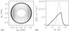 |
Fig. 8 Same as in Fig. 6, for the magnetosphere of Saturn. |
| In the text | |
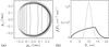 |
Fig. 9 Same as in Fig. 6, for the magnetosphere of an ultracool dwarf. |
| In the text | |
Current usage metrics show cumulative count of Article Views (full-text article views including HTML views, PDF and ePub downloads, according to the available data) and Abstracts Views on Vision4Press platform.
Data correspond to usage on the plateform after 2015. The current usage metrics is available 48-96 hours after online publication and is updated daily on week days.
Initial download of the metrics may take a while.